Climate: Observations,
projections and impacts:
China
Met Office
Simon N. Gosling, University of Nottingham Robert Dunn, Met Office
Fiona Carrol, Met Office Nikos Christidis, Met Office John Fullwood, Met Office Diogo de Gusmao, Met Office Nicola Golding, Met Office Lizzie Good, Met Office Trish Hall, Met Office Lizzie Kendon, Met Office John Kennedy, Met Office Kirsty Lewis, Met Office Rachel McCarthy, Met Office Carol McSweeney, Met Office Colin Morice, Met Office David Parker, Met Office Matthew Perry, Met Office Peter Stott, Met Office Kate Willett, Met Office
Myles Allen, University of Oxford
Nigel Arnell, Walker Institute, University of Reading Dan Bernie, Met Office
Richard Betts, Met Office
Niel Bowerman, Centre for Ecology and Hydrology Bastiaan Brak, University of Leeds
John Caesar, Met Office
Andy Challinor, University of Leeds Rutger Dankers, Met Office Fiona Hewer, Fiona's Red Kite
Chris Huntingford, Centre for Ecology and Hydrology Alan Jenkins, Centre for Ecology and Hydrology
Nick Klingaman, Walker Institute, University of Reading Kirsty Lewis, Met Office
Ben Lloyd-Hughes, Walker Institute, University of Reading Jason Lowe, Met Office
Rachel McCarthy, Met Office
James Miller, Centre for Ecology and Hydrology Robert Nicholls, University of Southampton
Maria Noguer, Walker Institute, University of Reading Friedreike Otto, Centre for Ecology and Hydrology Paul van der Linden, Met Office
Rachel Warren, University of East Anglia
The country reports were written by a range of climate researchers, chosen for their subject expertise, who were drawn from institutes across the UK. Authors from the Met Office and the University of Nottingham collated the contributions in to a coherent narrative which was then reviewed. The authors and
Developed at the request of:
Research conducted by:
China
We have reached a critical year in our response to climate change. The decisions that we made in Cancún put the UNFCCC process back on track, saw us agree to limit temperature rise to 2 °C and set us in the right direction for reaching a climate change deal to achieve this. However, we still have considerable work to do and I believe that key economies and major emitters have a leadership role in ensuring a successful outcome in Durban and beyond. To help us articulate a meaningful response to climate change, I believe that it is important to have a robust scientific assessment of the likely impacts on individual countries across the globe. This report demonstrates that the risks of a changing climate are wide-ranging and that no country will be left untouched by climate change.
I thank the UK’s Met Office Hadley Centre for their hard work in putting together such a comprehensive piece of work. I also thank the scientists and officials from the countries included in this project for their interest and valuable advice in putting it together. I hope this report will inform this key debate on one of the greatest threats to humanity.
The Rt Hon. Chris Huhne MP, Secretary of State for Energy and Climate Change
There is already strong scientific evidence that the climate has changed and will continue to change in future in response to human activities. Across the world, this is already being felt as changes to the local weather that people experience every day. Our ability to provide useful information to help everyone understand how their environment has changed, and plan for future, is improving all the time. But there is still a long way to go. These reports – led by the Met Office Hadley Centre in collaboration with many institutes and scientists around the world – aim to provide useful, up to date and impartial information, based on the best climate science now available. This new scientific material will also contribute to the next assessment from the Intergovernmental Panel on Climate Change. However, we must also remember that while we can provide a lot of useful information, a great many uncertainties remain. That’s why I have put in place a long-term strategy at the Met Office to work ever more closely with scientists across the world. Together, we’ll look for ways to combine more and better observations of the real world with improved computer models of the weather and climate; which, over time, will lead to even more detailed and confident advice being issued.
Introduction
Understanding the potential impacts of climate change is essential for informing both adaptation strategies and actions to avoid dangerous levels of climate change. A range of valuable national studies have been carried out and published, and the Intergovernmental Panel on Climate Change (IPCC) has collated and reported impacts at the global and regional scales. But assessing the
amount of information about past climate change and its future impacts has been available at
Each report contains:
data on extreme events.
Fourth Assessment Report from the IPCC.
Dangerous Climate Change programme (AVOID) and supporting literature.
1
Summary
Climate observations
Warming has been widespread over China over the period 1960 to 2010 with greater warming in winter then summer.
There has been a strong decrease in the frequency of cool nights since 1960 and an increase in the frequency of warm nights.
There has been a general increase in winter temperatures averaged over the country as a result of human influence on climate, making the occurrence of mild winter temperatures more frequent and cold winter temperatures less frequent.
Recent studies have found some evidence to suggest that annual total precipitation over China is increasing, as are days with heavy precipitation.
Climate change projections
For the A1B emissions scenario projected changes in temperature are higher over northern and western parts of the country, with changes of up to around 4.5°C. In the southeast, projected changes are typically around 3°C. There is good agreement between the models from the CMIP3 ensemble over most of China.
2
Climate change impacts projections
Crop yields
Although the picture is mixed, global- and regional-scale studies considered here generally project decreases in the yield of China’s major crops: rice, wheat, and most markedly of maize, as a consequence of climate change.
Some global-scale studies suggest that the magnitude of, and balance between, detrimental ozone effects and CO2 fertilisation may determine whether crop yield
losses or gains are realised under climate change.
Food security
China currently has very low levels of undernourishment. Global-scale studies of food security vary in their conclusions for China, however they generally project that the country will become less food secure with climate change.
National-scale studies confirm the uncertainty in food security estimates with some suggesting that China could experience large food shortages, while others suggest it may not face pressures on food security with climate change.
Water stress and drought
Global-scale studies included here agree that south-eastern China currently suffers from a moderate to high level of water stress.
Global- and regional-scale studies included here show no consensus as to the sign of change in drought or water stress in China with climate change.
However some global- and national-scale studies included here project that water stress could increase in China for global-mean warming scenarios of around 2°C, but may decrease under higher warming or higher emission scenarios, due to a projected increase in precipitation and runoff.
3
Pluvial flooding and rainfall
The IPCC AR4 noted the potential for increased precipitation over East Asia, and also an increase in extreme precipitation in parts of China.
Results from recent studies suggest that changes in precipitation extremes tend to be larger under higher emissions scenarios.
Fluvial flooding
Observations show that heavy precipitation events have increased over recent decades in parts of China, and flooding events have become more frequent in a number of river basins.
Climate change impact studies suggest that this trend could continue, although uncertainties are large, resulting in a wide spread in responses among different climate models.
Simulations by the AVOID programme show a general tendency towards higher flood risk in China, particularly later in the century and under the A1B scenario.
Tropical cyclones
There remains large uncertainty in the current understanding of how tropical cyclones might be affected by climate change.
There is relatively less uncertainty regarding the intensity of cyclones in the western Pacific basin, compared to their frequency. A number of global- and regional-scale studies included here project that cyclone intensity could increase considerably in the future in this basin. These increases in intensity could be greatest for the most severe cyclones, which could lead to large increases in cyclone damages in China.
China is particularly vulnerable to cyclone damages due to its high coastal population density and the valuable economic assets located in coastal regions.
Coastal regions
4
One study showed that based upon an analysis of 136 port cities, China was the country simulated to have the largest increase in exposure to SLR by 2070 relative to the present day.
5
Table of Contents
Chapter 1 – Climate Observations
... 9Rationale ... 10
Climate overview ... 12
Analysis of long-term features in the mean temperature ... 13
Temperature extremes ... 15
Recent extreme temperature events ... 17
Severe cold, January 2008 ... 17
Analysis of long-term features in moderate temperature extremes ... 17
Attribution of changes in likelihood of occurrence of seasonal mean temperatures ... 23
Winter 2007/08 ... 23
Precipitation extremes ... 25
Recent extreme precipitation events ... 27
Drought, May - November 2006 ... 27
Flooding, June-July 2007 ... 27
Analysis of long-term features in precipitation ... 27
Storms ... 31
Recent storm events ... 33
Tropical Storm Bilis, July 2006 ... 33
Summary ... 34
Methodology annex ... 35
Recent, notable extremes ... 35
Observational record ... 36
Analysis of seasonal mean temperature ... 36
Analysis of temperature and precipitation extremes using indices ... 37
Presentation of extremes of temperature and precipitation ... 47
Attribution ... 51
References ... 54
Acknowledgements ... 59
Chapter 2 – Climate Change Projections
... 61Introduction ... 62
Climate projections ... 64
Summary of temperature change in China ... 65
Summary of precipitation change in China ... 65
Chapter 3 – Climate Change Impact Projections
... 67Introduction ... 68
Aims and approach ... 68
Impact sectors considered and methods ... 68
Supporting literature ... 69
AVOID programme results ... 69
Uncertainty in climate change impact assessment ... 70
6
Crop yields ... 79
Headline... 79
Supporting literature ... 79
Introduction ... 79
Assessments that include a global or regional perspective ... 81
National-scale or sub-national scale assessments ... 87
AVOID programme ... 87
Methodology ... 87
Food security ... 91
Headline... 91
Supporting literature ... 91
Introduction ... 91
Assessments that include a global or regional perspective ... 91
National-scale or sub-national scale assessments ... 102
Water stress and drought ... 105
Headline... 105
Supporting literature ... 105
Introduction ... 105
Assessments that include a global or regional perspective ... 106
National-scale or sub-national scale assessments ... 114
AVOID Programme Results ... 116
Methodology ... 116
Results ... 117
Pluvial flooding and rainfall ... 119
Headline... 119
Supporting literature ... 119
Introduction ... 119
Assessments that include a global or regional perspective ... 119
National-scale or sub-national scale assessments ... 121
Fluvial flooding ... 122
Headline... 122
Supporting literature ... 122
Introduction ... 122
Assessments that include a global or regional perspective ... 123
National-scale or sub-national scale assessments ... 124
AVOID programme results ... 125
Methodology ... 125
Tropical cyclones ... 128
Headline... 128
Supporting literature ... 128
Introduction ... 128
Assessments that include a global or regional perspective ... 128
National-scale or sub-national scale assessments ... 134
Coastal regions ... 135
7
Supporting literature ... 135
Assessments that include a global or regional perspective ... 135
National-scale or sub-national scale assessments ... 146
9
10
Rationale
Present day weather and climate play a fundamental role in the day to day running of society. Seasonal phenomena may be
advantageous and depended upon for sectors such as farming or tourism. Other events, especially extreme ones, can sometimes have serious negative impacts posing risks to life and
infrastructure and significant cost to the economy. Understanding the frequency and magnitude of these phenomena, when they pose risks or when they can be advantageous and for which sectors of society, can significantly improve societal resilience.
In a changing climate it is highly valuable to understand possible future changes in both potentially hazardous events and those reoccurring seasonal events that are depended upon by sectors such as agriculture and tourism. However, in order to put potential future changes in context, the present day must first be well understood both in terms of common seasonal phenomena and extremes.
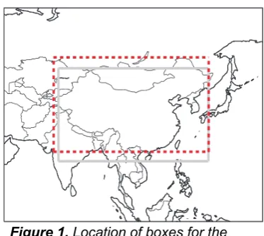
[image:15.595.334.521.113.280.2]The purpose of this chapter is to summarise the weather and climate from 1960 to present day. This begins with a general climate overview including an up to date analysis of changes in surface mean temperature. These changes may be the result of a number of factors including climate change, natural variability and changes in land use. There is then a focus on extremes of temperature, precipitation and storms selected from 2000 onwards, reported in the World Meteorological Organization (WMO) Annual Statement on the Status of the Global Climate and/or the Bulletin of the American Meteorological Society (BAMS) State of the Climate reports. This is followed by a discussion of changes in moderate extremes from 1960 onwards using an updated version of the HadEX extremes database (Alexander et al., 2006) which categorises extremes of temperature and precipitation. These are core climate variables which have received significant effort from the climate research community in terms of data acquisition and processing and for which it is possible to produce long high quality records for monitoring. No new analysis is included for storms (see the methodology section that follows for background). For seasonal temperature extremes, an attribution analysis then puts the seasons with highlighted extreme events into context of the recent climate versus a hypothetical climate in the absence of anthropogenic emissions (Christidis
11
et al., 2011). It is important to note that we carry out our attribution analyses on seasonal mean temperatures over the entire country. Therefore these analyses do not attempt to attribute the changed likelihood of individual extreme events. The relationship between extreme events and the large scale mean temperature is likely to be complex, potentially being influenced by inter alia circulation changes, a greater expression of natural internal variability at smaller scales, and local processes and feedbacks. Attribution of individual extreme events is an area of developing science. The work presented here is the foundation of future plans to systematically address the region’s present and projected future weather and climate, and the associated impacts.
12
Climate overview
China is a vast country on the eastern seaboard of Asia, extending between latitudes 20-50°N and including both long stretches of coastline and regions that are huge distances from any sea. Topography ranges from coastal lowlands in the east to high plateaux and
mountains in central and western regions. The climates of China are therefore complex and diverse. A phenomenon that steers the climate of much of China is the ‘Asiatic Monsoon’ in which, in summer, moist winds blow onshore from the Pacific (and Indian) Oceans towards low atmospheric pressure that develops over the hot Asian interior. These warm moist winds bring most of China’s rainfall. Conversely, in winter, very cold and dry winds blow outwards from the huge high atmospheric pressure system that develops over Siberia and central Asia.
The climate of the relatively low-lying eastern side of China can be divided into three latitudinal bands, each containing a section of the Pacific coastline. Annual average
temperatures range from 4°C at Harbin in the north-east to 22°C at Guangzhou (Canton) in the south-east. In north-eastern China winters are very cold with frequent light snow and typical January daily temperature maxima ranging from 2°C at Beijing (40°N) to -13°C at Harbin (46°N). Summers are warm and humid but with unreliable rainfall and some drought years. Annual average rainfall at Beijing is 521 mm. Further south in central-eastern China there is more precipitation (annual average rainfall 1112mm at Shanghai) and, although the main wet season is summer, winter is more changeable than further north with alternating mild and cold spells bringing some rain and some snow. South-eastern China is the warmest and wettest part of China in summer, with particularly heavy rainfall along the coast (annual average rainfall 1683mm at Guangzhou). Winters here are mild.
Inland southern China towards the borders with Vietnam and Laos is hilly or mountainous but still has mild or warm winters with very little precipitation. Only rarely does cold air
13
winters are cold or very cold, sometimes made more hazardous by dust-laden strong winds. Annual precipitation is low (Urumqi 236 mm); nonetheless, towards the north of Inner Mongolia the ground is snow covered for up to 150 days per year.
Typhoons are frequent between July and October in south-east coast regions and can cause wind damage and very heavy rainfall for several consecutive days, which can lead to
flooding. Occasionally, typhoons move further north to affect the central eastern coast. Other disruptive weather events in China include droughts, snow storms and extremes of cold (particularly away from the south) and extremes of heat (particularly over the western desert plains).
Analysis of long-term features in the mean temperature
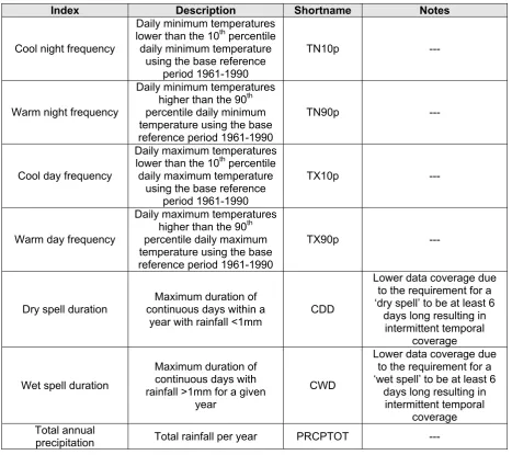
CRUTEM3 data (Brohan et al., 2006) have been used to provide an analysis of mean temperatures from 1960 to 2010 over China using the median of pairwise slopes method to fit the trend (Sen, 1968; Lanzante, 1996). The methods are fully described in the
methodology section. In agreement with increasing global average temperatures (Sánchez-Lugo et al., 2011), there is a widespread warming signal over China, consistent with
previous studies (Cruz et al., 2007). This signal is more robust and spatially consistent over winter (December to February) than in summer (June to August) as shown in Figure 2. For the summer, while warming is predominant, there are mixed signals and low confidence in a high proportion of grid boxes. For winter there is a far more spatially coherent signal of warming and confidence is high for the vast majority of grid boxes. This is consistent with previous studies which find that temperature has increased more in winter than summer (Zhai and Pan, 2003) and that there are regional differences in the level of warming. Regionally averaged trends (over grid boxes included in the red dashed box in Figure 1) calculated by the median of pairwise slopes show warming with high confidence as the 5th to
95th percentiles of the slope are of the same sign. There is stronger warming during winter at
0.37 oC per decade (5th to 95th percentile of slopes: 0.21 to 0.54 oC per decade) than during
14
15
Temperature extremes
Both hot and cold temperature extremes can place many demands on society. While seasonal changes in temperature are normal and indeed important for a number of societal sectors (e.g. tourism, farming etc.), extreme heat or cold can have serious negative impacts. Importantly, what is ‘normal’ for one region may be extreme for another region that is less well adapted to such temperatures.
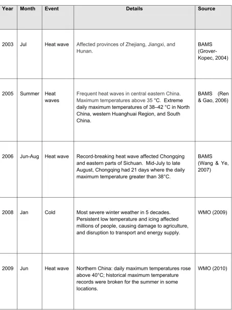
Table1 shows selected extreme events since 2000 that are reported in WMO Statements on Status of the Global Climate and/or BAMS State of the Climate reports. The severe winter of 2008 is highlighted below as an example of a recent extreme temperature event that
16
Year Month Event Details Source
2003 Jul Heat wave Affected provinces of Zhejiang, Jiangxi, and Hunan.
BAMS (Grover-Kopec, 2004)
2005 Summer Heat waves
Frequent heat waves in central eastern China. Maximum temperatures above 35 °C. Extreme daily maximum temperatures of 38–42 °C in North China, western Huanghuai Region, and South China.
BAMS (Ren & Gao, 2006)
2006 Jun-Aug Heat wave Record-breaking heat wave affected Chongqing and eastern parts of Sichuan. Mid-July to late August, Chongqing had 21 days where the daily maximum temperature greater than 38°C.
BAMS (Wang & Ye, 2007)
2008 Jan Cold Most severe winter weather in 5 decades. Persistent low temperature and icing affected millions of people, causing damage to agriculture, and disruption to transport and energy supply.
WMO (2009)
2009 Jun Heat wave Northern China: daily maximum temperatures rose above 40°C; historical maximum temperature records were broken for the summer in some locations.
[image:21.595.68.523.87.695.2]WMO (2010)
17
Recent extreme temperature events
Severe cold, January 2008
The severe winter in China in January 2008 was the worst winter weather experienced for half a century, with over 78 million people affected by the freezing temperatures and heavy snow (WMO, 2009). The average temperature in China during the winter months was
4.4°C making it the coldest winter since 1986/87 (Guo et al., 2009). Record breaking conditions were experienced where, averaged across southern China, 19 successive days occurred with a daily mean temperature of below 1°C. In addition to this, an accumulated mean snowfall of 42.4 mm was recorded (Rogers et al., 2009).
Extreme low temperatures, freezing rain, and snow persisted over most of southern China from 10th January to 2nd February, leading to the deaths of 107 people, and over US$15
billion in damage (Guo et al., 2009). These conditions affected millions of people through damage to agriculture, and disruption to transport, energy supply and power transmission (WMO, 2009).
The severe winter weather across much of China and central Asia was attributed to Eurasia’s largest January snow cover extent on record, where snow covered 1.3 million square kilometres across 15 provinces in southern China (WMO, 2009).
Analysis of long-term features in moderate temperature
extremes
GHCND data (Durre et al., 2010) have been used to update the HadEX extremes analysis for China from 1960 to 2010 using daily maximum and minimum temperatures. Here we discuss changes in the frequency of cool days and nights and warm days and nights which are moderate extremes. Cool days/nights are defined as being below the 10th percentile of
daily maximum/minimum temperature and warm days/nights are defined as being above the 90th percentile of the daily maximum/minimum temperature. The methods are fully described
in the methodology section.
18
and also to the south west, around the Himalayas. South-eastern regions, where there are a larger number of stations for each grid box, show a smaller trend.
On average there is a decrease in the number of cool days, with higher confidence in the signal over most of the west and northeast compared to the south and east. These latter areas have a smaller signal, and the area around the Guizhou region shows a small increase. Similar to cool nights, there is a stronger signal towards the Himalayas although station density is low here. The increase in the number of warm days is much more uniform in magnitude and high confidence in the signal is widespread. These findings are consistent with previous studies (Zhai and Pan, 2003; You et al., 2010).
22
Figure 3. Change in cool nights (a,b), warm nights (c,d), cool days (e,f) and warm days (g,h) for China over the period 1960 to 2010 relative to 1961-1990 from the GHCND dataset (Durre,et al., 2010). a,c,e,g) Grid box decadal trends. Grid boxes outlined in solid black contain at least 3 stations and so are likely to be more representative of the wider grid box. Trends are fitted using the median of pairwise slopes method (Sen, 1968; Lanzante, 1996). Higher confidence in a long-term trend is shown by a black dot if the 5th to 95th percentile slopes are of the same sign. Differences in spatial coverage occur because each index has its own decorrelation length scale (see the methodology section). b,d,f,h) Area averaged annual time series for 73.125o to 133.12o E and 21.25o to 53.75o N as
shown by the green box on the map and red box in Figure 1. Thin and thick black lines show the monthly and annual variation respectively. Monthly (orange) and annual (blue) trends are fitted as described above. The decadal trend and its 5th to 95th percentile confidence intervals are stated along with the change over the period for which data are available. All the trends have higher
23
Time-series from the regional averages have been calculated for China, as shown in Figure 3. There is a strong increase with high confidence that the trend is different from zero in the numbers of warm nights and warm days since the 1990s, consistent with the maps. A decrease in the number of cool nights is shown but the signal is smaller for cool day
frequency, matching the mixed signal and mixed confidence levels seen in Figure 3. These findings are broadly consistent with previous studies (Zhai and Pan, 2003; You et al., 2010). The severe winter of 2008 can be seen in the cool days and cool nights time-series as a spike corresponding to the green vertical line. The annual regional averages for the nights terminate earlier than for the days because although there are sufficient data to create some monthly regional averages, there are insufficient to create annual ones for these indices.
Attribution of changes in likelihood of occurrence of
seasonal mean temperatures
Today’s climate covers a range of likely extremes. Recent research has shown that the temperature distribution of seasonal means would likely be different in the absence of anthropogenic emissions (Christidis et al., 2011). Here we discuss the seasonal means, within which the highlighted extreme temperature event occurs, in the context of recent climate and the influence of anthropogenic emissions on that climate. The methods are fully described in the methodology section.
Winter 2007/08
The distributions of the winter mean regional temperatures in recent years in the presence and absence of anthropogenic forcings are shown in Figure 4. Analyses with two
independent coupled atmosphere and ocean general circulation models (HadGEM1 and MIROC) suggest that human influences on the climate have shifted the distribution towards higher temperatures than would be expected under natural influences alone. Considering the average over the entire region, the 2007/08 winter is not exceptionally cold, as it lies in the central sector, albeit the cooler half, of the temperature distributions for the climate
influenced by anthropogenic forcings. It is also considerably warmer than the winter of
1944/95, which is the coldest in the CRUTEM3 dataset and lies in the cold tail of the both the distribution affected by anthropogenic factors and that with natural factors only. In the
24
average. Notably, the warmest winter in CRUTEM3, 1998/1999, is more consistent with a winter temperature distribution under anthropogenic influences than natural ones.
The attribution results shown here refer to temperature anomalies averaged over the entire region and over an entire season, whereas the actual extreme event highlighted had a shorter duration and affected a smaller region.
Figure 4. Distributions of the December-January-February mean temperature anomalies (relative to 1961-1990) averaged over a region centred on China (75-133 oE, 18-50 oN – as shown in Figure 1) including (red lines) and excluding (green lines) the influence of anthropogenic forcings. The
25
Precipitation extremes
Precipitation extremes, either excess or deficit, can be hazardous to human health, societal infrastructure, and livestock and agriculture. While seasonal fluctuations in precipitation are normal and indeed important for a number of societal sectors (e.g. tourism, farming etc.), flooding or drought can have serious negative impacts. These are complex phenomena and often the result of accumulated excesses or deficits or other compounding factors such as spring snow-melt, high tides/storm surges or changes in land use. The analysis section below deals purely with precipitation amounts.
26
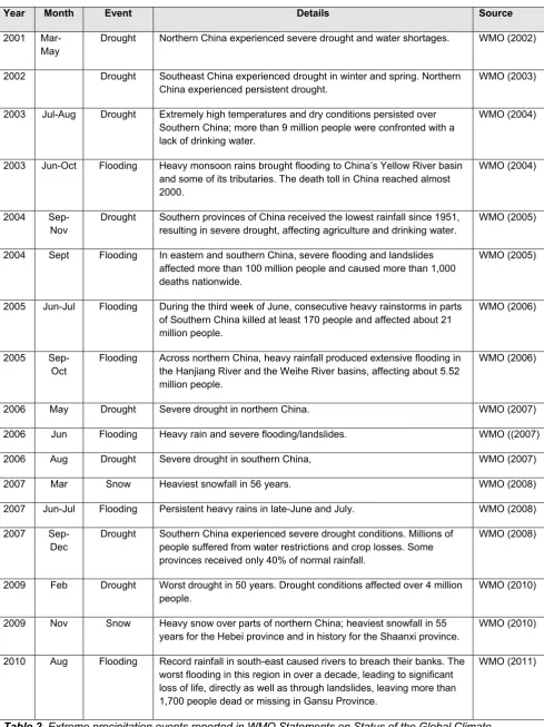
Year Month Event Details Source
2001 Mar-May
Drought Northern China experienced severe drought and water shortages. WMO (2002) 2002 Drought Southeast China experienced drought in winter and spring. Northern
China experienced persistent drought.
WMO (2003) 2003 Jul-Aug Drought Extremely high temperatures and dry conditions persisted over
Southern China; more than 9 million people were confronted with a lack of drinking water.
WMO (2004)
2003 Jun-Oct Flooding Heavy monsoon rains brought flooding to China’s Yellow River basin and some of its tributaries. The death toll in China reached almost 2000.
WMO (2004)
2004 Sep-Nov
Drought Southern provinces of China received the lowest rainfall since 1951, resulting in severe drought, affecting agriculture and drinking water.
WMO (2005) 2004 Sept Flooding In eastern and southern China, severe flooding and landslides
affected more than 100 million people and caused more than 1,000 deaths nationwide.
WMO (2005)
2005 Jun-Jul Flooding During the third week of June, consecutive heavy rainstorms in parts of Southern China killed at least 170 people and affected about 21 million people.
WMO (2006)
2005 Sep-Oct
Flooding Across northern China, heavy rainfall produced extensive flooding in the Hanjiang River and the Weihe River basins, affecting about 5.52 million people.
WMO (2006)
2006 May Drought Severe drought in northern China. WMO (2007) 2006 Jun Flooding Heavy rain and severe flooding/landslides. WMO ((2007) 2006 Aug Drought Severe drought in southern China, WMO (2007) 2007 Mar Snow Heaviest snowfall in 56 years. WMO (2008) 2007 Jun-Jul Flooding Persistent heavy rains in late-June and July. WMO (2008) 2007
Sep-Dec
Drought Southern China experienced severe drought conditions. Millions of people suffered from water restrictions and crop losses. Some provinces received only 40% of normal rainfall.
WMO (2008)
2009 Feb Drought Worst drought in 50 years. Drought conditions affected over 4 million people.
WMO (2010) 2009 Nov Snow Heavy snow over parts of northern China; heaviest snowfall in 55
years for the Hebei province and in history for the Shaanxi province.
WMO (2010) 2010 Aug Flooding Record rainfall in south-east caused rivers to breach their banks. The
worst flooding in this region in over a decade, leading to significant loss of life, directly as well as through landslides, leaving more than 1,700 people dead or missing in Gansu Province.
[image:31.595.69.559.85.739.2]WMO (2011)
27
Recent extreme precipitation events
Drought, May - November 2006
During May, northern China suffered from severe drought conditions that damaged 12% of the nation’s agriculture (WMO, 2007). This was followed by further drought in southern China in August during which 18 million people were affected, causing significant economic losses as well as severe shortages in drinking water (WMO, 2007). From June through to mid November, the Yangtze River valley endured dry conditions as average precipitation was the second lowest since 1951, causing record low river levels (Wang, 2007).
Flooding, June-July 2007
Heavy rains caused devastating floods in the Huaihe River Valley in late June and July (Suda et al., 2008). The BBC reported that Hunan province was placed on high alert after four successive days of rain caused the Xiangjiang River to swell to its highest level in 20 years (BBC, 2007). This flood was believed to be the worst in the region since 1954 (WMO, 2008), killing over 500 people and affecting more than 100 million (CRED, 2007). It was also reported by the BBC that nearly 20,000 hectares of cropland were flooded and 3,000 houses destroyed in the southern province of Guizhou (BBC, 2007). The total cost in damages was estimated at over US$ 4 million (CRED, 2007).
Analysis of long-term features in precipitation
29
Figure 5. The change in annual total rainfall (a,b), the annual number of continuous dry days (c,d) and the annual number of continuous wet days (e,f) over the period 1960-2010. The maps and time series have been created in exactly the same way as Figure 3. Only annual regional averages are shown in b,d,f). The dotted lines in b,d,f) indicate that there is lower confidence that the trends are different from zero. The time series for the indices terminate before the notable events for 2006 and 2007 outlined earlier and so no comment can be made about their magnitude compared to past extreme events.
The signal from the precipitation indices is restricted to the eastern parts of China due to limited station coverage and a shorter decorrelation length scale for these indices (see the methodology section for details). Over the analysed period (1960-2009), using the GHCND dataset as shown in Figure 5, overall the signal for the total precipitation is mixed. There are increasing precipitation totals in the northeast and southeast but decreases centrally.
Confidence is low in these signals for the most part. The increase in total precipitation in the south east agrees with the results of Hu et al. (2003) and You et al. (2010). The data
30
There is a more coherent pattern to the trends in the number of continuous dry days, with the central and north-eastern regions showing a clear decrease with high confidence, agreeing with the study of You et al. (2010). However the number of stations present within these grid boxes is on the whole small.
Recent studies have found some evidence to suggest that annual total precipitation is increasing, as are days with heavy precipitation and a decrease in consecutive dry days. The greatest increases in precipitation have been found in the Yangtze River basin, south-eastern and north-western China, with changes of up to 30%, whilst decreases in
31
Storms
Storms can be very hazardous to all sectors of society. They can be small with localised impacts or spread across multiple states. There is no systematic observational analysis included for storms because, despite recent progress (Peterson et al., 2011; Cornes & Jones, 2011), wind data are not yet adequate for worldwide robust analysis (see methodology
section). Further progress awaits studies of the more reliable barometric pressure data through the new 20th Century Reanalysis (Compo et al., 2011) and its planned successors.
32
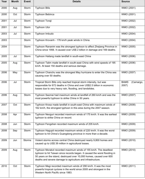
Year Month Event Details Source
2000 Aug Storm Typhoon Bilis WMO (2001) 2000 Oct Storm Typhoon Bebinca WMO (2001) 2001 Jul Storm Typhoon Toraji WMO (2002) 2001 Jul Storm Typhoon Utor WMO (2002) 2003 Jul Storm Typhoon Imbudo WMO (2004) 2003 Storm Typhoon Krovanh - 176 km/h peak winds in China. WMO (2004) 2004 Storm Typhoon Rananim was the strongest typhoon to affect Zhejiang Province in
China since 1956. It caused over US$ 2 billion in damage and 169 deaths.
WMO (2005) 2005 Jul Storm Typhoon Haitang made landfall in south-east China WMO (2006) 2005 Aug Storm Typhoon Talim made landfall in south-east China with wind speeds of 195
km/h. At least 150 deaths and serious damage.
WMO (2006) 2006 May Storm Typhoon Chanchu was the strongest May hurricane to enter the China sea
causing over 50 deaths.
WMO (2007) 2006 Jul Storm Tropical Storm Bilis only reached tropical storm intensity, but was
responsible for 672 deaths in China and over US$2.5 billion in economic losses due to very heavy rain, flooding, and landslides.
BAMS (Camargo, 2007)
2006 Aug Storm Typhoon Saomai had maximum winds at landfall of 260 km/h and was the most powerful typhoon to strike China in 50 years.
WMO (2007) 2007 Oct Storm Typhoon Krosa made landfall in south-east China with maximum winds of
162 km/h, the strongest typhoon in this area during the 2007 season.
WMO (2008) 2008 Apr Storm Typhoon Neoguri recorded maximum winds of 175 km/h. It was the earliest
typhoon to strike China on record.
WMO (2009) 2008 Jun Storm Typhoon Fengshen recorded maximum winds of 205 km/h. WMO (2009) 2008 Sep Storm Typhoon Hagupit recorded maximum winds of 220 km/h. It was the worst
typhoon to hit China’s Guangdong province in more than a decade.
WMO (2009) 2009 Jun Storms Violent storms across central China destroyed nearly 9,800 homes and
caused up to US$ 39 million in agricultural losses.
WMO (2010) 2009 Aug Storm Typhoon Morakot recorded maximum winds of 155 km/h. The deadliest
typhoon to hit Taiwan since records began. It caused the worst flooding in 50 years on the island, destroyed over 10,000 homes, caused over 600 deaths and severe damage to agriculture and infrastructure.
WMO (2010)
2010 Oct Storm Typhoon Megi recorded maximum winds of 290 km/h. It was the most powerful tropical cyclone in the world since 2005 and strongest in the Western North Pacific since 1983.
[image:37.595.69.541.97.682.2]WMO (2011)
33
Recent storm events
Tropical Storm Bilis, July 2006
Bilis made landfall in China on 14th July and, although only reaching tropical storm intensity, was responsible for 672 deaths in China and over US$2.5 billion in economic losses due to very heavy rain, flooding, and landslides (Camargo, 2007). The BBC reported that the Chinese government evacuated over quarter of a million people from the southern province of Fujian in preparation for the storms arrival (BBC, 2006a). There was disruption to
34
Summary
The main features seen in observed climate over China from this analysis are:
There has been widespread warming over China over the period 1960 to 2010 with greater warming in winter then summer.
There has been a strong decrease in the frequency of cool nights since 1960 and an increase in the frequency of warm nights.
There has been a general increase in winter temperatures averaged over the country as a result of human influence on climate, making the occurrence of mild winter temperatures more frequent and cold winter temperatures less frequent.
35
Methodology annex
Recent, notable extremes
In order to identify what is meant by ‘recent’ events the authors have used the period since 1994, when WMO Status of the Global Climate statements were available to the authors. However, where possible, the most notable events during the last 10 years have been chosen as these are most widely reported in the media, remain closest to the forefront of the memory of the country affected, and provide an example likely to be most relevant to today’s society. By ‘notable’ the authors mean any event which has had significant impact either in terms of cost to the economy, loss of life, or displacement and long term impact on the population. In most cases the events of largest impact on the population have been chosen, however this is not always the case.
Tables of recent, notable extreme events have been provided for each country. These have been compiled using data from the World Meteorological Organisation (WMO) Annual Statements on the Status of the Global Climate. This is a yearly report which includes contributions from all the member countries, and therefore represents a global overview of events that have had importance on a national scale. The report does not claim to capture all events of significance, and consistency across the years of records available is variable. However, this database provides a concise yet broad account of extreme events per country. This data is then supplemented with accounts from the monthly National Oceanic and
Atmospheric Administration (NOAA) State of the Climate reports which outline global extreme events of meteorological significance.
36
Our search for data has not been exhaustive given the number of countries and events included. Although there are a wide variety of sources available, for many events, an official account is not available. Therefore figures given are illustrative of the magnitude of impact only (references are included for further information on sources). It is also apparent that the reporting of extreme events varies widely by region, and we have, where possible, engaged with local scientists to better understand the impact of such events.
The aim of the narrative for each country is to provide a picture of the social and economic vulnerability to the current climate. Examples given may illustrate the impact that any given extreme event may have and the recovery of a country from such an event. This will be important when considering the current trends in climate extremes, and also when examining projected trends in climate over the next century.
Observational record
In this section we outline the data sources which were incorporated into the analysis, the quality control procedure used, and the choices made in the data presentation. As this report is global in scope, including 23 countries, it is important to maintain consistency of methodological approach across the board. For this reason, although detailed datasets of extreme temperatures, precipitation and storm events exist for various countries, it was not possible to obtain and incorporate such a varied mix of data within the timeframe of this project. Attempts were made to obtain regional daily temperature and precipitation data from known contacts within various countries with which to update existing global extremes databases. No analysis of changes in storminess is included as there is no robust historical analysis of global land surface winds or storminess currently available.
Analysis of seasonal mean temperature
37
High confidence is assigned to any trend value for which the 5th to 95th percentiles of the
pairwise slopes are of the same sign as the trend value and thus inconsistent with a zero trend.
Analysis of temperature and precipitation extremes using indices
In order to study extremes of climate a number of indices have been created to highlight different aspects of severe weather. The set of indices used are those from the World Climate Research Programme (WCRP) Climate Variability and Predictability (CLIVAR) Expert Team on Climate Change Detection and Indices (ETCCDI). These 27 indices use daily rainfall and maximum and minimum temperature data to find the annual (and for a subset of the indices, monthly) values for, e.g., the ‘warm’ days where daily maximum temperature exceeds the 90th percentile maximum temperature as defined over a 1961 to
38
Index Description Shortname Notes
Cool night frequency
Daily minimum temperatures lower than the 10th percentile daily minimum temperature
using the base reference period 1961-1990
TN10p ---
Warm night frequency
Daily minimum temperatures higher than the 90th percentile daily minimum temperature using the base reference period 1961-1990
TN90p ---
Cool day frequency
Daily maximum temperatures lower than the 10th percentile daily maximum temperature
using the base reference period 1961-1990
TX10p ---
Warm day frequency
Daily maximum temperatures higher than the 90th percentile daily maximum temperature using the base reference period 1961-1990
TX90p ---
Dry spell duration
Maximum duration of continuous days within a
year with rainfall <1mm CDD
Lower data coverage due to the requirement for a ‘dry spell’ to be at least 6
days long resulting in intermittent temporal
coverage
Wet spell duration
Maximum duration of continuous days with rainfall >1mm for a given
year
CWD
Lower data coverage due to the requirement for a ‘wet spell’ to be at least 6
days long resulting in intermittent temporal
coverage Total annual
[image:43.595.65.533.100.515.2]precipitation Total rainfall per year PRCPTOT --- Table 4. Description of ETCCDI indices used in this document.
A previous global study of the change in these indices, containing data from 1951-2003 can be found in Alexander et al. 2006, (HadEX; see http://www.metoffice.gov.uk/hadobs/hadex/). In this work we aimed to update this analysis to the present day where possible, using the most recently available data. A subset of the indices is used here because they are most easily related to extreme climate events (Table 4).
Use of HadEX for analysis of extremes
39
developed and maintained on behalf of the ETCCDI by the Climate Research Branch of the Meteorological Service of Canada. Given the timeframe of this project it was not possible to obtain sufficient station data to create updated HadEX indices to present day for a number of countries: Brazil; Egypt; Indonesia; Japan (precipitation only); South Africa; Saudi Arabia; Peru; Turkey; and Kenya. Indices from the original HadEX data-product are used here to show changes in extremes of temperature and precipitation from 1960 to 2003. In some cases the data end prior to 2003. Table 5 summarises the data used for each country. Below, we give a short summary of the methods used to create the HadEX dataset (for a full description see Alexander et al. 2006).
To account for the uneven spatial coverage when creating the HadEX dataset, the indices for each station were gridded, and a land-sea mask from the HadCM3 model applied. The interpolation method used in the gridding process uses a decorrelation length scale (DLS) to determine which stations can influence the value of a given grid box. This DLS is calculated from the e-folding distance of the individual station correlations. The DLS is calculated separately for five latitude bands, and then linearly interpolated between the bands. There is a noticeable difference in spatial coverage between the indices due to these differences in decorrelation length scales. This means that there will be some grid-box data where in fact there are no stations underlying it. Here we apply black borders to grid-boxes where at least 3 stations are present to denote greater confidence in representation of the wider grid-box area there. The land-sea mask enables the dataset to be used directly for model comparison with output from HadCM3. It does mean, however, that some coastal regions and islands over which one may expect to find a grid-box are in fact empty because they have been treated as sea.
Data sources used for updates to the HadEX analysis of extremes
We use a number of different data sources to provide sufficient coverage to update as many countries as possible to present day. These are summarised in Table 2. In building the new datasets we have tried to use exactly the same methodology as was used to create the original HadEX to retain consistency with a product that was created through substantial international effort and widely used, but there are some differences, which are described in the next section.
40
Differences in the patterns of the trends in the indices can arise because the individual stations used to create the gridded results are different from those in HadEX, and the quality control procedures used are also very likely to be different. Countries where we decided to use HadEX data despite the existence of more recent data are Egypt and Turkey.
GHCND:
The Global Historical Climate Network Daily data has near-global coverage. However, to ensure consistency with the HadEX database, the GHCND stations were compared to those stations in HadEX. We selected those stations which are within 1500m of the stations used in the HadEX database and have a high correlation with the HadEX stations. We only took the precipitation data if its r>0.9 and the temperature data if one of its r-values >0.9. In addition, we required at least 5 years of data beyond 2000. These daily data were then converted to the indices using the fclimdex software.
ECA&D and SACA&D:
The European Climate Assessment and Dataset and the Southeast Asian Climate Assessment and Dataset data are pre-calculated indices comprising the core 27 indices from the ETCCDI as well as some extra ones. We kindly acknowledge the help of Albert Klein Tank, the KNMI1 and the BMKG2 for their assistance in obtaining these data.
Mexico:
The station data from Mexico has been kindly supplied by the SMN3 and Jorge Vazquez.
These daily data were then converted to the required indices using the Fclimdex software. There are a total of 5298 Mexican stations in the database. In order to select those which have sufficiently long data records and are likely to be the most reliable ones we performed a cross correlation between all stations. We selected those which had at least 20 years of data post 1960 and have a correlation with at least one other station with an r-value >0.95. This resulted in 237 stations being selected for further processing and analysis.
1Koninklijk Nederlands Meteorologisch Instituut – The Royal Netherlands Meteorological Institute
2
Badan Meteorologi, Klimatologi dan Geofisika – The Indonesian Meteorological, Climatological and Geophysical Agency
3
41 Indian Gridded:
42 Coun tr y Region bo x (re d da she d boxes in Fig. 1 and on each map at begin ning of cha pt er ) Data sour ce (T = temperature, P = precipitation) Period of data cov erage (T = temp erat ure, P = pre cipitati on) Indices inclu ded (se e Tabl e 4 for details)
Temporal resolution av
ailable Not es Argentin a 73.125 to 54. 375 o W, 21.25 to 56 .25 o S Matilde Ru st icu cci (T,P) 1960 -20 10 (T ,P) TN10 p, TN9 0p , TX10p, TX90 p, PRCPT O T, C DD, CW D annu al Aus tralia 114.37 5 to 15 5.625
o E
, 1 1. 25 to 4 3. 75
o S
GHCND (T,P ) 1960 -20 10 (T ,P) TN10 p, TN9 0p , TX10p, TX90 p, PRCPT O T, C DD, CW D monthly, se aso na l a nd annu al Land -sea ma sk has been adapte d to inclu de Ta sm ania an d the area ar ound Brisb ane Banglad esh 88.125 to 91. 875 o E, 21.25 to 26.25 o N Indian Gri dde d data (T,P) 1960 -20 07 (P ), 1970 -20 09 (T ) TN10 p, TN9 0p , TX10p, TX90 p, PRCPT O T, C DD, CW D monthly, se aso na l a nd annu al Interpolate d from India n Gridded da ta Braz il 73.125 to 31. 875 o W, 6.25
o N
to
33.75
o S
HadEX (T,P) 1960 -20 00 (P ) 2002 (T) TN10 p, TN9 0p , TX10p, TX90 p, PRCPT O T, C DD, CW D annu al Spatial cove rage is poor Ch in a 73.125 to 13 3. 125 o E, 21.25 to 53.75 o N GH CN D (T,P ) 1960 -19 97 (P ) 1960 -20 03 (Tmin ) 1960 -20 10 (Tma x ) TN10 p, TN9 0p , TX10p, TX90 p, PRCPT O T, C DD, CW D monthly, se aso na l a nd annu al Preci pitation has very po or covera ge beyond 1997 except in 20 03 -04, an d no data at all in 2000 -02, 20 05 -11 Egypt 24.375 to 35. 625 o E, 21.25 to 31.25 o N HadEX (T,P) No data TN10 p, TN9 0p , TX10p, TX90 p, PRCPT O T, annu al There are no data for Egyp t so all grid -box values ha ve been inte rpolate d from station s in Jo rdan, Israel, Libya and Sudan Fran ce 5.625
o W
to
9
.3
75
o E
, 4 1. 25 to 5 1. 25
o N
43 Germ any 5.625 to 16.8 75
o E,
46.25
to
56.2
5
o N
ECA&D (T,P) 1960 -20 10 (T ,P) TN10 p, TN9 0p , TX10p, TX90 p, PRCPT O T, C DD, CW D monthly, se aso na l a nd annu al India 69.375 to 99. 375 o E, 6.25 to 36.25
o N
Indian Gri dde d data (T,P) 1960 -20 03 (P ), 1970 -20 09 (T ) TN10 p, TN9 0p , TX10p, TX90 p, PRCPT O T, C DD, CW D monthly, se aso na l a nd annu al Indone sia 95.625 to 14 0. 625 o E, 6.25
o N
to
1
1.
25
o S
HadEX (T,P) 1968 -20 03 (T ,P) TN10 p, TN9 0p , TX10p, TX90 p, PRCPT O T, annu al Spatial cove rage is poor Italy 5.625 to 16.8 75
o E,
36.25
to
46.2
5
o N
ECA&D (T,P) 1960 -20 10 (T ,P) TN10 p, TN9 0p , TX10p, TX90 p, PRCPT O T, C DD, CW D monthly, se aso na l a nd annu al Land -sea ma sk has been adapte d to improve cove rage of Italy Ja pa n 129.37 5 to 14 4.375
o E
, 3 1. 25 to 4 6. 25
o N
HadEX (P) GH CN D (T ) 1960 -20 03 (P ) 1960 -20 00 (Tmin ) 1960 -20 10 (Tma x ) TN10 p, TN9 0p , TX10p, TX90 p, PRCPT O T, monthly, se aso na l a nd annu al (T), annu al (P) Kenya 31.875 to 43. 125 o E, 6.25
o N
to 6 .2 5 o S HadEX (T,P) 1960 -19 99 (P ) TN10 p, TN9 0p , TX10p, TX90 p, PRCPT O T annu al There are no temperature data for Kenya and so grid-box valu es have been inte rpol ated from nei ghbo urin g Uga nda and the Unite d Re publi c of Tanzania. Re gional ave rag es in clud e grid -boxe s fro m outside Ke nya that enabl e co ntin uation to 200 3 Mexico 118.12 5 to 88 .125 o W, 13.75 to 33 .75 o N Ra w station data from the Servicio Meteorológi co Na cion al (SMN ) (T,P) 1960 -20 09 (T ,P) TN10 p, TN9 0p , TX10p, TX90 p, PRCPT O T, C DD, CW D monthly, se aso na l a nd annu al 237/52 98 stat ions sele cted. Non uniform spati al coverage. Dro p in T and P covera ge in 2009. Peru 84.735 to 65. 625 o W, 1.25
o N
t
o
18.75
o S
44 Ru ssi a We st Ru ssi a 28.125 to 10 6. 875 o E, 43.75 to 78.75 o N, Ea st R us si a 103.12 5 to 18 9.375
o E
, 4 3. 75 to 7 8. 75
o N
ECA&D (T,P) 1960 -20 10 (T ,P) TN10 p, TN9 0p , TX10p, TX90 p, PRCPT O T, C DD, CW D monthly, se aso na l a nd annu al Cou ntry split for presentatio n purp oses only. Saudi Arabi a 31.875 to 54. 375 o E, 16.25 to 33.75 o N HadEX (T,P) 1960 -20 00 (T ,P) TN10 p, TN9 0p , TX10p, TX90 p, PRCPT O T annu al Spatial cove rage is poor South Africa 13.125 to 35. 625 o W, 21.25 to 36 .25 o S HadEX (T,P) 1960 -20 00 (T ,P) TN10 p, TN9 0p , TX10p, TX90 p, PRCPT O T, C DD, CW D annu al --- Rep ubli c of Korea 125.62 5 to 12 9.375
o E
, 3 3. 75 to 3 8. 75
o N
HadEX (T,P) 1960 -20 03 (T ,P) TN10 p, TN9 0p , TX10p, TX90 p, PR C PTOT, CD D annu al There are too few data poi nts for CWD to calculate trend s or regio nal times eries Spain 9.375
o W
to
1
.8
75
o E
, 3 6. 25 to 4 3. 75
o N
ECA&D (T,P) 1960 -20 10 (T ,P) TN10 p, TN9 0p , TX10p, TX90 p, PRCPT O T, C DD, CW D monthly, se aso na l a nd annu al Turkey 24.375 to 46. 875 o E, 36.25 to 43.75 o N HadEX (T,P) 1960 -20 03 (T ,P) TN10 p, TN9 0p , TX10p, TX90 p, PRCPT O T, C DD, CW D annu al Inter m ittent cover age in CW D and CDD with no re gio nal avera ge beyond 20 00
United Kingdom
9.375
o W
to
1
.8
75
o E
, 5 1. 25 to 5 8. 75
o N
ECA&D (T,P) 1960 -20 10 (T ,P) TN10 p, TN9 0p , TX10p, TX90 p, PRCPT O T, C DD, CW D monthly, se aso na l a nd annu al
United States
45
Quality control and gridding procedure used for updates to the HadEX analysis of extremes
In order to perform some basic quality control checks on the index data, we used a two-step process on the indices. Firstly, internal checks were carried out, to remove cases where the 5 day rainfall value is less than the 1 day rainfall value, the minimum T_min is greater than the minimum T_max and the maximum T_min is greater than the maximum T_max. Although these are physically impossible, they could arise from transcription errors when creating the daily dataset, for example, a misplaced minus sign, an extra digit appearing in the record or a column transposition during digitisation. During these tests we also require that there are at least 20 years of data in the period of record for the index for that station, and that some data is found in each decade between 1961 and 1990, to allow a reasonable estimation of the climatology over that period.
Weather conditions are often similar over many tens of kilometres and the indices calculated in this work are even more coherent. The correlation coefficient between each station-pair combination in all the data obtained is calculated for each index (and month where
appropriate), and plotted as a function of the separation. An exponential decay curve is fitted to the data, and the distance at which this curve has fallen by a factor 1/e is taken as the decorrelation length scale (DLS). A DLS is calculated for each dataset separately. For the GHCND, a separate DLS is calculated for each hemisphere. We do not force the fitted decay curve to show perfect correlation at zero distance, which is different to the method employed when creating HadEX. For some of the indices in some countries, no clear decay pattern was observed in some data sets or the decay was so slow that no value for the DLS could be determined. In these cases a default value of 200km was used.
We then perform external checks on the index data by comparing the value for each station with that of its neighbours. As the station values are correlated, it is therefore likely that if one station measures a high value for an index for a given month, its neighbours will also be measuring high. We exploit this coherence to find further bad values or stations as follows. Although raw precipitation data shows a high degree of localisation, using indices which have monthly or annual resolution improves the coherence across wider areas and so this
neighbour checking technique is a valid method of finding anomalous stations.
46
differences in elevation or topography into account when comparing neighbours, as we are not comparing actual values, but rather deviations from the mean value.
All stations which are within the DLS distance are investigated and their anomalised values noted. We then calculate the weighted median value from these stations to take into account the decay in the correlation with increasing distance. We use the median to reduce the sensitivity to outliers.
If the station value is greater than 7.5 median-absolute-deviations away from the weighted median value (this corresponds to about 5 standard deviations if the distribution is Gaussian, but is a robust measure of the spread of the distribution), then there is low confidence in the veracity of this value and so it is removed from the data.
To present the data, the individual stations are gridded on a 3.75o x 2.5o grid, matching the
output from HadCM3. To determine the value of each grid box, the DLS is used to calculate which stations can reasonably contribute to the value. The value of each station is then weighted using the DLS to obtain a final grid box value. At least three stations need to have valid data and be near enough (within 1 DLS of the gridbox centre) to contribute in order for a value to be calculated for the grid point. As for the original HadEX, the HadCM3 land-sea mask is used. However, in three cases the mask has been adjusted as there are data over Tasmania, eastern Australia and Italy that would not be included otherwise (Figure 6).
47
Presentation of extremes of temperature and precipitation
Indices are displayed as regional gridded maps of decadal trends and regional average time-series with decadal trends where appropriate. Trends are fitted using the median of pairwise slopes method (Sen 1968, Lanzante 1996). Trends are considered to be significantly
different from a zero trend if the 5th to 95th percentiles of the pairwise slopes do not
encompass zero. This is shown by a black dot in the centre of the grid-box or by a solid line on time-series plots. This infers that there is high confidence in the sign (positive or negative) of the sign. Confidence in the trend magnitude can be inferred by the spread of the 5th to 95th
percentiles of the pairwise slopes which is given for the regional average decadal trends. Trends are only calculated when there are data present for at least 50% of years in the period of record and for the updated data (not HadEX) there must be at least one year in each decade.
Due to the practice of data-interpolation during the gridding stage (using the DLS) there are values for some grid boxes when no actually station lies within the grid box. There is more confidence in grid boxes for which there are underlying data. For this reason, we identify those grid boxes which contain at least 3 stations by a black contour line on the maps. The DLS differs with region, season and index which leads to large differences in the spatial coverage. The indices, by their nature of being largely threshold driven, can be intermittent over time which also effects spatial and temporal coverage (see Table 1).
Each index (and each month for the indices for which there is monthly data) has a different DLS, and so the coverage between different indices and datasets can be different. The restrictions on having at least 20 years of data present for each input station, at least 50% of years in the period of record and at least one year in each decade for the trending calculation, combined with the DLS, can restrict the coverage to only those regions with a dense station network reporting reliably.
Each country has a rectangular region assigned as shown by the red dashed box on the map in Figure 1 and listed in Table 2, which is used for the creation of the regional average. This is sometimes identical to the attribution region shown in grey on the map in Figure 1. This region is again shown on the maps accompanying the time series of the regional averages as a reminder of the region and grid boxes used in the calculation. Regional averages are created by weighting grid box values by the cosine of their grid box centre latitude. To ensure consistency over time a regional average is only calculated when there are a sufficient number of grid boxes present. The full-period median number of grid-boxes present is
48
of the median number of grid boxes present for any one year to calculate a regional average. For regions with six or fewer median grid boxes this is relaxed to 50%. These limitations ensure that a single station or grid box which has a longer period of record than its neighbours cannot skew the timeseries trend. So sometimes there may be grid-boxes present but no regional average time series. The trends for the regional averages are calculated in the same way as for the individual grid boxes, using the median of pairwise slopes method (Sen 1968, Lanzante 1996). Confidence in the trend is also determined if the 5th to 95th percentiles of the pairwise slopes are of the same sign and thus inconsistent with a
50
Figure 7. Examples of the plots shown in the data section. Left: From ECA&D data between 1960-2010 for the number of warm nights, and Right: from HadEX data (1960-2003) for the total
precipitation. A full explanation of the plots is given in the text below.
51
base period of 1961-1990 (except the Indian gridded data which use a 1971 to 1990 period), both in HadEX and in the new data acquired for this project. Therefore, for example, the percentage of nights exceeding the 90th percentile for a temperature is 10% for that period.
There are two influences on whether a grid box contains a value or not – the land-sea mask, and the decorrelation length scale. The land-sea mask is shown in Figure 6. There are grid boxes which contain some land but are mostly sea and so are not considered. The
decorrelation length scale sets the maximum distance a grid box can be from stations before no value is assigned to it. Grid boxes containing three or more stations are highlighted by a thick border. This indicates regions where the value shown is likely to be more representative of the grid box area mean as opposed to a single station location.
On the maps for the new data there is a box indicating which grid boxes have been extracted to calculate the area average for the time series. This box is the same as shown in Figure 1 at the beginning of each country’s document. These selected grid boxes are combined using area (cosine) weighting to calculate the regional average (both annual [thick lines] and monthly [thin lines] where available). Monthly (orange) and annual (blue) trends are fitted to these time series using the method described above. The decadal trend and total change over the period where there are data are shown with 5th to 95th percentile confidence intervals in parentheses. High confidence, as determined above, is shown by a solid line as opposed to a dotted one. The green vertical lines on the time series show the dates of some of the notable events outlined in each section.
Attribution
Regional distributions of seasonal mean temperatures in the 2000s are computed with and without the effect of anthropogenic influences on the climate. The analysis considers
52
Observations of land temperature come from the CRUTEM3 gridded dataset (Brohan et al., 2006) and model simulations from two coupled GCMs, namely the Hadley Centre HadGEM1 model (Martin et al., 2006) and version 3.2 of the MIROC model (K-1 Developers, 2004). The use of two GCMs helps investigate the sensitivity of the results to the model used in the analysis. Ensembles of model simulations from two types of experiments are used to partition the temperature response to external forcings between its anthropogenic and natural components. The first experiment (ALL) simulates the combined effect of natural and anthropogenic forcings on the climate system and the second (ANTHRO) includes
anthropogenic forcings only. The difference of the two gives an estimate of the effect of the natural forcings (NAT). Estimates of the effect of internal climate variability are derived from long control simulations of the unforced climate. Distributions of the regional summer mean temperature are computed as follows:
a) A global optimal fingerprinting analysis (Allen and Tett, 1999; Allen and Stott, 2003) is first carried out that scales the global simulated patterns (fingerprints) of climate change attributed to different combinations of external forcings to best match them to the observations. The uncertainty in the scaling that originates from internal variability leads to samples of the scaled fingerprints, i.e. several realisations that are plausibly consistent with the observations. The 2000-2009 decade is then extracted from the scaled patterns and two samples of the decadal mean temperature averaged over the reference region are then computed with and without human influences, which
provide the Probability Density Functions (PDFs) of the decadal mean temperature attributable to ALL and NAT forcings.
b) Model-derived estimates of noise are added to the distributions to take into account the uncertainty in the simulated fingerprints.