A nested recursive logit model for route choice analysis

Munich Personal RePEc Archive

A nested recursive logit model for route

choice analysis

Mai, Tien and Frejinger, Emma and Fosgerau, Mogens

Department of Computer Science and Operational Research,

Universite de Montreal and CIRRELT, Canada, Department of

Computer Science and Operational Research, Universite de

Montreal and CIRRELT, Canada, Technical University of Denmark,

Denmark, and Royal Institute of Technology, Sweden

23 March 2015

Online at

https://mpra.ub.uni-muenchen.de/63161/

A nested recursive logit model for

route choice analysis

Tien Mai

Mogens Fosgerau

Emma Frejinger

March 22, 2015

Abstract

We propose a route choice model that relaxes the independence from irrelevant alternatives property of the logit model by allowing scale parameters to be link specific. Similar to the the recursive logit (RL) model proposed by Fosgerau et al. (2013), the choice of path is modelled as a sequence of link choices and the model does not require any sampling of choice sets. Furthermore, the model can be consistently estimated and efficiently used for prediction.

A key challenge lies in the computation of the value functions, i.e. the expected maximum utility from any position in the network to a destination. The value functions are the solution to a system of non-linear equations. We propose an iterative method with dynamic accuracy that allows to efficiently solve these systems.

We report estimation results and a cross-validation study for a real network. The results show that the NRL model yields sensible parameter estimates and the fit is significantly better than the RL model. Moreover, the NRL model outperforms the RL model in terms of prediction.

Keywords: route choice modelling; nested recursive logit; substitution pat-terns; value iterations; maximum likelihood estimation; cross-validation.

∗_{Department of Computer Science and Operational Research, Universit´e de Montr´eal}

and CIRRELT, Canada

†_{Technical University of Denmark, Denmark, and Royal Institute of Technology,}

1

Introduction

Discrete choice models are generally used for analyzing path choices in real networks based on revealed preference (RP) data. There are two main mod-elling issues associated with (i) estimating such models consistently and (ii) subsequently using them for prediction. First, choice sets of paths are un-known to the analyst and the set of all feasible paths for a given origin-destination pair cannot be enumerated. Second, path utilities may be cor-related, for instance, due to physical overlap in the network. As we explain below, there is currently no path choice model that can be consistently esti-mated and used for prediction, while avoiding the specification of choice sets and allowing for correlation due to path overlap. The nested recursive logit (NRL) model, proposed in this paper, fills this gap.

Most of the existing path choice models are based on choice sets of paths that need to be sampled before estimating or applying the model. Many dif-ferent algorithms exist for sampling choice sets (for reviews, see e.g. Frejinger et al., 2009, Prato, 2009) and they all correspond to importance sampling protocols where paths have non-equal probabilities of being sampled. Fre-jinger et al. (2009) show that utilities need to be corrected for the sampling of alternatives, which implies that only algorithms that allow computation of the path sampling probabilities can be used. Frejinger et al. (2009) use the logit (MNL) model but recently Guevara and Ben-Akiva (2013a) and Guevara and Ben-Akiva (2013b) have derived results for generalized extreme value (GEV) and mixed logit models, respectively. The sampling approach can be used to consistently estimate a path choice model, but it is still un-known how to use that model for prediction.

men-tioned earlier, the MEV models (e.g. link-nested logit) or the mixed logit models can be corrected. Lai and Bierlaire (2014) estimate a link-nested logit model using the results by Guevara and Ben-Akiva (2013a).

Recently, Fosgerau et al. (2013) proposed the recursive logit (RL) model where path choice is modelled as a sequence of link choices using a dynamic discrete choice framework. The RL model can be consistently estimated and used for prediction without sampling choice sets of paths. It is however equivalent to a MNL model over the set of all feasible paths. A correction attribute called link size was proposed that achieves an effect similar to the path size attribute in path choice models (Ben-Akiva and Bierlaire, 1999). These attributes correct the utilities for correlation but the models retain the independence of irrelevant alternatives (IIA) property, unless the path size/link size attributes are updated as utilities change (e.g. changes in link travel times).

In this paper we propose an extension of the RL model that allows path utilities to be correlated in a fashion similar to nested logit (Ben-Akiva, 1973, McFadden, 1978) and where links can have different scale parameters. The key challenge with this extension lies in the computation of the expected maximum utility from a current position in the network until the destination (value functions). A computational advantage of the RL model is that the value functions can be computed by solving a system of linear equations, which is fast and easy to do. In the case of the NRL, the value functions are a solution to a system of non-linear equations which is substantially more difficult to deal with. We propose an iterative method with dynamic accuracy to efficiently solve this equation system.

This paper makes a number of contributions. First we propose a model that can be consistently estimated and used for prediction without sampling choice sets while allowing the random terms to be correlated. Second, we provide illustrative examples and discuss substitution patterns in order to build an intuition on the properties of the model. Third, we propose an iterative method to solve for the value functions and we derive the analyt-ical gradient of the log-likelihood function for the case that the scales are functions of model parameters so that the NRL model can be efficiently esti-mated. Fourth, we provide estimation and cross-validation results for a real network using simulated and real observations. Finally, the estimation code is implemented in MATLAB and is freely available upon request.

and finally Section 7 concludes.

2

The nested recursive logit model

In the RL model (Fosgerau et al., 2013) the path choice problem is formu-lated as a sequence of link choices and modelled in a dynamic discrete choice framework. At each node the decision maker chooses the utility-maximizing outgoing link with link utilities given by the instantaneous utility and the expected maximum utility to the destination. The random terms of the instantaneous utilities are independently and identically distributed (i.i.d.) extreme value type I so that the model is equivalent to MNL. In this section we present the NRL model which relaxes the IIA property of MNL by assum-ing that the scales of random terms are non-equal across links. We derive the NRL model using the same notation as Fosgerau et al. (2013) (we refer the reader to that paper for a more detailed presentation of the notation). Even though the derivation of NRL is similar to the RL one, the resulting ex-pressions of the value functions and path choice probabilities have important differences.

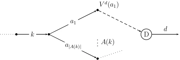
A directed connected graph (not assumed acyclic)G = (A,V) is consid-ered, where A and V are the sets of links and nodes, respectively. For each link k ∈ A, we denote the set of outgoing links from the sink node of k by

A(k). Moreover we associate an absorbing state with each destination by extending the network with dummy links d (see Figure 1). This is a link without successors so a trip stops once this state is reached. The set of all links is ˜A=A∪ {d}and the corresponding deterministic utility isv(d|k) = 0 for all k that have destination d as sink node. Given two links a, k ∈A˜, the following instantaneous utility is associated with action a∈A(k) of individ-ual n

un(a|k;β) =vn(a|k;β) +µkǫ(a) (1)

where β is a vector of parameters, ǫ(a) are i.i.d extreme value type I and

µk is a strictly positive scale parameter. We ensure that ǫ(a) have zero

mean by subtracting Euler’s constant. The deterministic term vn_{(a|k;β) is}

assumed negative for all links except the dummy link d. We emphasize the difference with the original RL model where scale parameters are assumed equal (µk = µ ∀k ∈ A). For notational simplicity, we omit an index for

individual n but note that the utilities can be individual specific.

The expected maximum utility from the sink node ofkto the destination is the value function Vd_{(k;β). The superscript d indicates that the value}

D d

k

a1

a|A(k)|

Vd_(a

1)

··

·_A(k)

Figure 1: Illustration of notation

Vd_{(k;β) is recursively defined by Bellman’s equation}

Vd(k;β) = Eh max

a∈A(k) v(a|k;β) +V

d_{(a;β) +µ}

kǫ(a)i ∀k ∈A (2)

or equivalently

1

µk

Vd(k;β) =Eh max

a∈A(k)

1

µk

(v(a|k;β) +Vd(a;β)) +ǫ(a)i ∀k ∈A. (3)

For notational simplicity we omit from now on β from the value functions

V(.) and the utilities v(.).

Given these assumptions the probability of choosing link a given state k

is given by the MNL model

Pd(a|k) =δ(a|k) e

1

µk(v(a|k)+V d_(a))

P

a′_∈A(k)e

1

µk(v(a′|k)+Vd(a′))

=δ(a|k)eµk1 (v(a|k)+Vd(a)−Vd(k)) _{∀k, a∈A.}˜

(4)

Note that we includeδ(a|k) that equals one ifa∈A(k) and zero otherwise so that the probability is defined for all a, k ∈A˜(we recall that ˜A=A∪ {d}). Since we assume that the random terms in (1) are distributed i.i.d. EV type I, the value functions (2) are given recursively by the logsum

1

µk

Vd(k) = ln X

a∈A(k)

eµk1 (v(a|k)+V d_(a))

∀k ∈A (5)

and Vd_{(d) = 0 by assumption. Similar to Fosgerau et al. (2013) we can write}

(5) as

eµk1 V d_(k)

=

(P

a∈Aδ(a|k)e

(v(a|k)+V d(a))

µk _∀k∈A

and define a matrix Md_(|A˜_{| × |A}˜_{|) and a vector z}d_(|A˜_{| ×1) with entries}

M_kad =δ(a|k)ev(µka|k)_{, z}d

k =e

V(k)

µk _{, k, a∈A.}˜ ₍₇₎

The key issue here compared to the RL model is that we do not end up with a system of linear equations. Indeed, the value functions are the solutions to the following system of non-linear equations

z_kd=

(P

a∈AMkad(zad)µa/µk ∀k∈A

1 k=d, (8)

where the non-linearity arises due to the scale parametersµknot being equal.

The probability of a pathσdefined by a sequence of linksσ = [k0, k1, . . . , kI]

is

P(σ) =

I−1

Y

i=0

e

1

µk_i(v(ki+1|ki)+V d_(k

i+1)−Vd(ki))

. (9)

Unlike the RL model, the link specific value functions do not cancel out due to the scale parameters. This implies that the path choice probabilities are computationally more costly to evaluate.

We note that if the network contains cycles, the RL and NRL model allow for paths to contain loops (Akamatsu, 1996, Fosgerau et al., 2013, discuss this in more detail). The probability of paths with loops depend on the data and network structure. For the data used in this paper, Fosgerau et al. (2013) report that paths with loops have a very small probability.

Finally we note that the IIA property does not hold in the NRL model. Consider the ratio of the choice probabilities of two paths σ1 = [k1, . . . , kI1]

and σ2 = [h1, . . . , hI2] connecting just one origin-destination pair

P(σ1)

P(σ2)

=

QI1−1

i=1 e

1

µk_i(v(ki+1|ki)+V d_(k

i+1)−Vd(ki))

QI2−1

i=1 e

1

µh_i(v(hi+1|hi)+Vd(hi+1)−Vd(hi))

. (10)

When the scales µk=µ∀k∈A, the value function terms cancel out and the

3

Illustrative examples and substitution

pat-terns

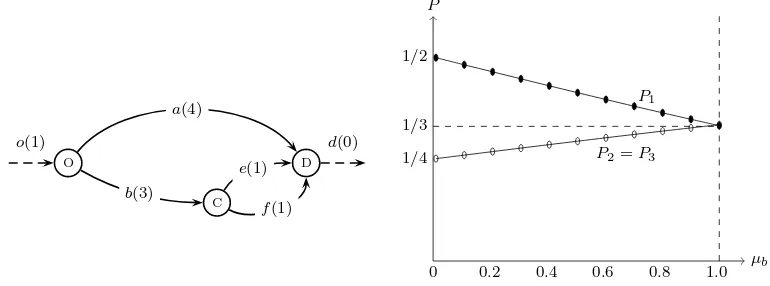
Similar to several studies in the literature (e.g. Ben-Akiva and Bierlaire, 1999), we use a simple three path network shown in 2 to illustrate why it is important to allow for correlated utilities. There are three paths from o

to d (link o is the origin and link d is the destination dummy link): [o, a, d], [o, b, e, d], [o, b, f, d]. We number these paths 1,2 and 3 and the corresponding path probabilities are P1,P2 and P3, respectively. The only attribute in the

instantaneous utility is link length and the values are given in the parentheses on each arc. In order to compute path probabilities we choose a length parameter ˜β =−1.

When the scales of random terms are equal over links µk =µ, the model

corresponds the RL and P1 = P2 = P3 = 1/3. When the network has

a perfect nested structure as this one (each path in the network belongs to exactly one nest when defined by physical overlap), the NRL model is equivalent to a nested logit model. We can illustrate this by fixing all the scale parameters to 1 except µb that we vary over the interval (0,1]. The

path probabilities are plotted in the graph on the right hand side in Figure 2.

O

C

D a(4)

b(3)

e(1)

f(1)

d(0)

o(1)

µb

P

0 0.2 0.4 0.6 0.8 1.0 1/3

1/2

1/4 P2=P3

P1

Figure 2: Classic three paths example network

In order to build intuition on the substitution patterns implied by the NRL model, we provide three more examples. The first is shown in Figure 3 which also has a simple nested structure. There are 4 nodes A, B, C, D

and 9 links. Moreover, there are 6 possible paths from o to d: [o, a, a1, d],

[o, a, a2, d], [o, a, a3, d], [o, b, b1, d], [o, b, b2, d] and [o, b, b3, d] and we number

these paths as 1, 2, 3, 4, 5 and 6, respectively.

any link in the network, the probabilities of the remaining feasible paths will increase by the same proportion (for example if we remove link a2, the

probabilities of path [o, a, a3, d] and path [o, b, b3, d] increase but they are

still equal). For the NRL model, the scales of random terms are assigned different values. We assign a scale of 0.5 for links a, a scale of 0.8 for links b

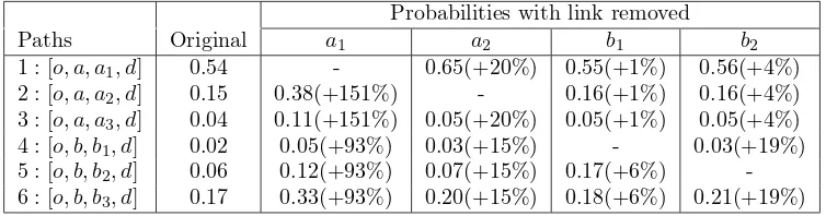
and a scale of 1.0 for the others. Similar to an example in Train (2003), we illustrate substitution patterns by removing in turn links a1, a2, b1, b2 and

present changes in probabilities in Table 1.

A

B

C

D a(1)

b(2)

a1(1)

a2(2)

a3(3)

b1(2)

b2(1.5)

b3(1)

d(0)

o(1) N1 N2

1 2 3 4 5 6

paths nests

Figure 3: Example network with perfect nested structure

Probabilities with link removed

Paths Original a1 a2 b1 b2

1 : [o, a, a1, d] 0.54 - 0.65(+20%) 0.55(+1%) 0.56(+4%)

2 : [o, a, a2, d] 0.15 0.38(+151%) - 0.16(+1%) 0.16(+4%)

3 : [o, a, a3, d] 0.04 0.11(+151%) 0.05(+20%) 0.05(+1%) 0.05(+4%)

4 : [o, b, b1, d] 0.02 0.05(+93%) 0.03(+15%) - 0.03(+19%)

5 : [o, b, b2, d] 0.06 0.12(+93%) 0.07(+15%) 0.17(+6%)

-6 : [o, b, b3, d] 0.17 0.33(+93%) 0.20(+15%) 0.18(+6%) 0.21(+19%)

Table 1: Change in probability when link is removed (example network with perfect nested structure)

We note that the probabilities for paths [o, a, a1, d], [o, a, a2, d], [o, a, a3, d]

rise by the same proportions whenever one link is removed from the network. This is also the case for the three paths [o, b, b1, d], [o, b, b2, d] and [o, b, b2, d].

As expected, the IIA property holds between paths within the same nest but not for paths in different nests. For example, when link a1 is removed, the

probabilities of the paths in the first nest rise by 151% while the paths in the second nest rise by 93%.

A

B

C

D E

a(1)

b(2)

a1(1)

a2(2)

a3(2)

f(2)

b1(1)

b2(1.5)

b3(1)

e(1)

d(0)

o(1) N1 N2

1 2 3 4 5 6

paths nests

Figure 4: Example network with cross-nested structure

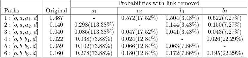
before. We note that the absolute values of choice probabilities change but the substitution pattern remains proportional.

Probabilities with link removed

Paths Original a1 a2 b1 b2

1 : [o, a, a1, d] 0.487 - 0.572(17.52%) 0.504(3.48%) 0.522(7.27%)

2 : [o, a, a2, d] 0.140 0.298(113.38%) - 0.144(3.48%) 0.150(7.27%)

3 : [o, a, a3, d] 0.040 0.085(113.38%) 0.047(17.52%) 0.041(3.48%) 0.043(7.27%)

4 : [o, b, b1, d] 0.022 0.038(73.88%) 0.024(12.84%) - 0.026(22.29%)

5 : [o, b, b2, d] 0.059 0.102(73.88%) 0.066(12.84%) 0.063(7.86%)

-6 : [o, b, b3, d] 0.160 0.278(73.88%) 0.180(12.84%) 0.172(7.86%) 0.195(22.29%)

Table 2: Change in probability when link is removed (example network with perfect nested structure with link from B to C)

The network in Figure 3 is designed so that the paths can naturally be divided into separate nests. In the next example shown in Figure 4 we slightly modify the network so that paths have a cross-nested structure. More precisely, we add a node E that splits links a3 and b1 into two links. The

lengths of the paths in the new network do not change but the structure of the network is different since apart from the origin and destination, two paths [o, a, a3, e, d] and [o, a, b1, e, d] share link e. Furthermore, there is a new link

f going (backward) from node E to node A so that the expected maximum utilities from link a3 and b1 depend on the whole network.

We report probabilities for the 6 paths without loops: [o, a, a1, d], [o, a, a2, d],

[o, a, a3, e, d], [o, b, b1, e, d], [o, b, b2, d], [o, b, b3, d], which are numbered as 1, 2,

3, 4, 5 and 6, respectively. We keep the same scales as in the first example (i.e. µa = 0.5, µb = 0.8 and the other scale parameters are equal to one).

The changes in probabilities of the six paths when we remove in turn links

a3,b1 and f are reported in Table 3. We note that the substitution patterns

and 4 no longer change by the same proportion as the other paths in their respective nest.

Probabilities with link removed

Paths Original a1 b3 f

1 : [o, a, a1, d] 0.54 - 0.60(+12%) 0.54(+0.7%)

2 : [o, a, a2, d] 0.15 0.38(+150%) 0.17(+12%) 0.15(+0.7%)

3 : [o, a, a3, e, d] 0.05 0.11(+148%) 0.05(+11%) 0.04(-1.3%)

4 : [o, b, b1, e, d] 0.03 0.05(+86%) 0.05(+90%) 0.02(-6.7%)

5 : [o, b, b2, d] 0.06 0.12(+93%) 0.12(+91%) 0.06(+1.4%)

6 : [o, b, b3, d] 0.17 0.33(+93%) - 0.17(+1.4%)

Table 3: Change in probability when link is removed (example network with cross-nested structure)

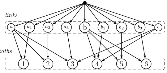
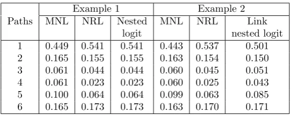
In order to compare the results with path based models we report prob-abilities given by the nested logit and link-nested logit (Vovsha and Bekhor, 1998) models in Table 4. The correlation structure given by the link-nested logit model is shown in Figure 5. For the nested models, the nesting param-eters take the same values as in the NRL mode, namely 0.8 for nest N1 and 0.5 for nest N2. The results show that for these examples, the probabilities of the nested model are identical to the NRL model and probabilities of the link-nested logit are slightly different from NRL. We note that the sums of the path probabilities for RL and NRL in the second example are slightly smaller than one, due to the cycle in the network.

In summary, the IIA property can be relaxed by assuming different scales. The resulting substitution pattern depends on the network structure. If the network has a perfect nested structure (e.g Figure 3) the NRL and nested logit models yield the same results.

b

a a1 a2 a3 b1 b2 b3 e

1 2 3 4 5 6

links

paths

Example 1 Example 2 Paths MNL NRL Nested MNL NRL Link

logit nested logit 1 0.449 0.541 0.541 0.443 0.537 0.501 2 0.165 0.155 0.155 0.163 0.154 0.150 3 0.061 0.044 0.044 0.060 0.045 0.051 4 0.061 0.023 0.023 0.060 0.025 0.043 5 0.100 0.064 0.064 0.099 0.063 0.085 6 0.165 0.173 0.173 0.163 0.170 0.171

Table 4: Path probabilities comparison

4

Computation of the value functions

The main challenge associated with the NRL model is to efficiently solve the large-scale system of system of non-linear equations (6). In the following we describe a value iteration approach that is efficient thanks to (i) a good initial solution and (ii) dynamic accuracy.

We define a matrixX(z) with entries

X(z)ka=zaµa/µk ∀k, a∈A˜ (11)

so that the Bellman equation (8) can be written as

z = [M ◦X(z)]e+b. (12)

b is a vector of size (|A˜| ×1) with zero values for all states except for the destination that equals 1,e is a vector of size (|A˜| ×1) with value one for all states and ◦ is the element-by-element product.

Value iterations are based on Equation (12). We start with an initial vector z0 _{and then for each iteration iwe compute a new vector}

zi+1 ←[M ◦X(zi)]e+b. (13) and iterate until a fixed point is found using ||zi+1 _−zi_||2 _{< γ for a given}

threshold γ > 0 as stopping criteria.1 _{It can be shown that if the Bellman}

equation has a solution, this method converges after a finite number of it-erations (see for instance Rust, 1987, 1988). The choice of initial vector is however important for the rate of convergence. We use the solution of the system of linear equations corresponding to the RL model (µk =µ ∀k ∈A)

which is fast to compute.

1_{The value functions can also be used in the stopping criteria i.e. the iteration stops}

whenPk∈A˜(V

i+1

(k)−Vi

(k))2

< γ′_{. The value functions have however larger magnitudes}

The proofs in the literature establishing the existence and uniqueness of a solution to Bellman’s equation use a discount factor less than one. In our case we do not discount future utilities and these proofs do not apply. Fosgerau et al. (2013) discuss this issue in more detail for the RL model. In essence, the existence of a solution depends on the balance between the number of paths connecting the nodes in the network and the size of the scaled instantaneous utilities. It is easy to find a feasible solution by using large enough magnitude of the β parameters.

Since the value functions depend on the parameter values, they need to be solved repeatedly when searching over the parameter space (maximum likelihood estimation). In order to decrease the computational time we use dynamic accuracy. More precisely, we update the thresholdγ in the iterations of the non-linear optimization algorithm so that higher accuracy is required close to optimum (γ decreases as the number of iterations of the non-linear optimization algorithm increases).

Before discussing the maximum likelihood estimation in more detail, we note that (12) can be written asF(z) = 0, whereF(z) = z−[M◦X(z)]e+b. A standard solver can be used e.g. fsolver in MATLAB or the Newton-GMRES method (for instance Kelley, 1995). We have tested these methods but found that they are not efficient for our application and that our approach works better.

5

Maximum likelihood estimation

There are several different ways of estimating a dynamic discrete choice model (Aguirregabiria and Mira, 2010), we adopt the nested fixed point algorithm of Rust (1987). This algorithm combines an outer iterative non-linear op-timization algorithm for searching over the parameter space with an inner algorithm for solving the value functions.2 _{The latter was the focus of the}

previous section and we now turn our attention to the definition of the log-likelihood (LL) function and the derivation of its gradient which allows us to use classic Hessian approximation such as BHHH and BFGS (see for instance Berndt et al., 1974, Nocedal and Wright, 2006).

The path probabilities are defined by (9) and contain scale parameters

2_{Another option is the algorithm proposed by Aguirregabiria and Mira (2002). The idea}

µk ∀k∈ A as well as the parameters β associated with the attributes of the

instantaneous utilities. Clearly, it is not possible to estimate all link-specific scale parameters for a real network and therefore we assume that they are a function of parameters β to be estimated µk(β). (We refer the reader to the

numerical results, Section 6, for an example.)

The LL function defined over the set of path observations n = 1, . . . , N

is

LL(β) =

N

X

n=1

lnP(σn, β) = N X n=1 In X t=0 1

µkt

(vn(kt+1|kt) +Vn(kt+1)−Vn(kt))

(14) and is very similar to the LL function of the RL model except that the value functions for the states along a path do not cancel out. Assuming a linear-in-parameters formulation of the instantaneous utilities, the gradient with respect to a given parameter βi is

∂LL(β)

βi = 1 N N X n=1

IXn−1

t=1

1

µkt

∂vn_(k t+1|kt)

∂βi

+∂V

n_(k t+1)

∂βi

− ∂V

n_(k t)

∂βi

− ∂µkt

µ2

kt∂βi

(vn(kt+1|kt) +Vn(kt+1) +Vn(kt))

and hence requires the first derivative of the value functions Vn_{(k), ∀k ∈A˜}

with respect to βi. We define φka = µa/µk and take the derivative of a

given value function zk as defined by (8) (without using the superscript for

destination d) and obtain

∂zk

∂βi

=X

a∈A

∂Mka

∂βi

zφka

a +Mkazaφka

φka

za

∂za

∂βi

+ ∂φka

∂βi

lnza

=X

a∈A

∂Mka

∂βi

zφka

a +Mkazaφka

∂φka

∂βi

lnza

+X

a∈A

Mkazaφka

φka za ∂za ∂βi . (15) We note that when the scales µk contain some model parameters, the

deriva-tive of each element of matrix M(β) with respect to a given parameter βi

is

∂Mka

∂βi

=δ(a|k)ev(µka|k)

∂v(a|k)

µk∂βi

−v(a|k) ∂µk

µ2

k∂βi

, k, a∈A.˜

We introduce two matrices, Gi _{and K of size |A˜| × |A˜|, which have the two}

sums of (15) as entries

Gi_ka= ∂Mka

∂βi

zφka

a +Mkazφaka

∂φka

∂βi

Kka=Mkazφaka

φka

za

, ∀k, a∈A.˜ (16)

This allows us to define the Jacobian of vector z as a system of linear equa-tions

∂z ∂βi

=Gie+K ∂z ∂βi

⇒ ∂z

∂βi

= (I−K)−1Gie, (17)

which in theory, can be solved very efficiently. Nevertheless, it is possible to use the fact that V(k) = µklnzk ∀k ∈ A˜ and derive the Jacobian of V

instead of z. In this case the gradient of V(k) with respect to a givenβi is

∂V(k)

∂βi

= ∂µk

∂βi

lnzk+

µk

zk

∂zk

∂βi

. (18)

Using (15) we get

∂V(k)

∂βi

=X

a∈A

S_kai +X

a∈A

Hka

∂V(a)

∂βi

+hk (19)

where

S_kai =µk

∂Mka

∂βi

zφka

a

zk

+µkMkaln(za)

zφka

a

zk

∂φka

∂βi

−Mkaln(za)

zφka

a

zk

∂µa

∂βi

and

Hka=Mka

zφka

a

zk

and hk =

∂µk

∂βi

lnzk.

We denote Si_{,H be two matrices of size|A}˜_{| × |A}˜_{|and h,V be two vectors of}

size |A˜| ×1 with entriesSi

ka,Hka,hk,V(k) for allk, a∈A˜, respectively. The

Jacobian of vector V can then be written as a system of linear equations

∂V ∂βi

= (I−H)−1(Sie+h). (20)

Although theoretically equivalent, we now discuss the numerical differ-ences between the two formulas (17) and (20) for computing the gradient of the value functions. We consider the definitions of the matrix K and H. za,

a ∈A˜are exponential functions of the value functions which are negative by assumption. The value of za may therefore be very close to zero. Since the

elements of matrix K can be written as Kka = φkaMkazaφka−1 (∀k, a ∈A˜) if

φka<1, the value of Kka can be very large, and ifφka>1,Kka can be very

also in matrix I−K) can lead to numerical issues when solving the system (17). Based on equation (8), each element of matrix H can be written as

Hka =

Mkazaφka

P

a′_∈A(k)Mka′zφka′

a′

= 1

1 +P_a′_∈A(k),a′_6=a

M_ka′z

φ ka′ a′

Mkazφkaa

∀k, a∈A, a˜ ∈A(k)

so that 0 < Hka < 1, meaning that the elements of matrix H are closer in

value, compared to matrixK. Therefore, using (20) to compute the gradient of LL function is better than (17) for numerical reasons. In summary, the analytical gradient of the LL function has a complicated form but can be efficiently computed by solving systems of linear equations.

6

Numerical results

In this section we present estimation and prediction results for four different models: the RL model with and without link size (LS) attribute and the NRL model, also with and without LS attribute. We use the same data as Fosgerau et al. (2013) (also used in Frejinger and Bierlaire, 2007, Mai et al., 2014) which has been collected in Borl¨ange, Sweden. The network is composed of 3077 nodes and 7459 links and is uncongested so travel times can be assumed static and deterministic. The sample consists of 1832 trips corresponding to simple paths with a minimum of five links. Moreover, there are 466 destinations, 1420 different origin-destination (OD) pairs and more than 37,000 link choices in this sample.

6.1

Model specifications

The same five attributes as Fosgerau et al. (2013) are used in the instanta-neous utilities. First, link travel time T T(a) of actiona. Second, a left turn dummy LT(a|k) that equals one if the turn angle from k toa is larger than 40 degrees and less than 177 degrees. Third, a u-turn dummy U T(a|k) that equals one if the turn angle is larger than 177. Fourth, a link constantLC(a). The fifth attribute is LS(a) (for a detailed description see Fosgerau et al., 2013) and it has been computed using a linear-in-parameters formulation of the aforementioned four attributes using parameters ˜βT T =−2.5, ˜βLT =−1,

˜

Even in this fairly small network there are more than 7000 links, so it is not possible to estimate link specific parameters. We therefore impose a constraint on the scale parameters µk > 0 by defining them as a function

of link attributes. More precisely, µk = eλk where λk = ωxk, ω is a vector

of parameters and xk a vector of attributes associated with link k. This

assumption ensures that (i) the estimation problem is unconstrained and (ii) we can use the analytical gradient (18). Note that if all the parameters in

λk are zero, the scales are equal to one for all linksk ∈A˜, meaning that the

NRL model becomes the RL model. As much as data allows, it is possible to elaborate on the specification of the scale parameters. For example, by including different attributes in the exponential function or by estimating link specific scales parameters for some links in the network.

For the numerical results presented in this paper we use three link specific attributes: travel time, LS and the number of outgoing linksOL(k) = |A(k)|. Accordingly, λk is

λk =ωT TT T(k) +ωLSLS(k) +ωOLOL(k). (21)

We do not use a link constant since it has the same value for all links, the rationale behind using it in the instantaneous utilities is to penalize paths with many crossings (links). Note that this is not a regression model, it is simply a specification of the scale parametersµkthat enter the instantaneous

utility functions.

To summarize, the deterministic utilities for four different model specifi-cations with respect to link a given link k are

vRL(a|k;β) = vNRL(a|k;β) = βT TT T(a) +βLTLT(a|k) +βLCLC(a)

+βU TU T(a|k)

vRL-LS(a|k;β) =vNRL-LS(a|k;β) = βT TT T(a) +βLTLT(a|k) +βLCLC(a)

+βU TU T(a|k) +βLSLS(a)

and the instantaneous utilities are

uRL_{(a|k;β) = v}RL_{(a|k;β) +µǫ(a)}

uRL-LS(a|k;β) = vRL-LS(a|k;β) +µǫ(a)

uNRL(a|k;β, ω) = vNRL(a|k;β) +eλk_ǫ(a)

uNRL-LS(a|k;β, ω) = vNRL-LS(a|k;β) +eλk_ǫ(a).

6.2

Estimation results

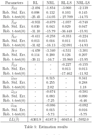
Theβestimates have their expected signs and are highly significant. _bωLS and

b

ωOL are significant and negative while ωbT T is not significantly different from

zero when the LS attribute is included in the instantaneous utilities. The LS attribute corresponds to expected normalized flows and takes positive values but is numerically close to zero for a majority of the links in the network.

b

ωLS andbωOLindicate that the scales are inversely related to flow and number

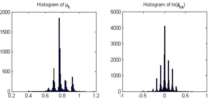
of outgoing links; links with more flow and more outgoing links have smaller variance of the error terms than links with less flow and fewer outgoing links. It is not straightforward to analyze the resulting scale parameters based on _bω. We therefore provide two histograms in Figure 6 showing the distri-bution of µk and lnφka = lnµ_µa_k over the links in the network for the NRL-LS

model. The graph on the left shows that the values of µk vary over the links

in the network which ensures that IIA does not hold (the average value of

µk is 0.78). The peaks in the distribution are due to the attribute number of

outgoing links OL(k) which take discrete values. We note that a few links have values larger than one: this is consistent with utility maximization and does not imply counter intuitive path probabilities. The graph on the right shows the distribution of lnφka which is quite symmetric around 0 (the

av-erage value of φka is 1.03). The symmetry can be explained by the attribute

OL(k). Consider the u-turn linka′ _{of linka∈A(k). Since linkk anda}′ _have

the same sink node we have OL(k) = OL(a′_{). For our data this results in}

values of µk numerically close to µa′ and thus

φkaφaa′ = µa

µk

µa′

µa

≈1

or equivalently

lnφka+ lnφaa′ ≈0.

Figure 6: Histogram of µk and lnφka for NRL-LS

Before comparing prediction results in the following section we make some remarks concerning the estimation. We use a basic trust region algorithm with the BHHH method for approximating the Hessian and the code is im-plemented in MATLAB (and available upon request). We use the iterative method with dynamic accuracy for the computation of the value functions (see Section 4). We note that if we use an initial vector as a solution of the system of linear equations, about 100 iterations is enough for a high precision (γ′ _{= 10}−8_{) but we need about 200 iterations for the same precision when the}

initial vector is the unit vector (all the elements are equal to one). Moreover, using only 50 iterations in the beginning of the optimization (corresponding to a precisionγ′ _{∈[1,10]) and switching to the high precisionγ}′ _{= 10}−8 _when

the norm of the gradient of the log-likelihood function is less than 10−3 _we

were able to double the speed of the estimation.

6.3

Prediction results

0 5 10 15 20 25 30 35 40 3.15

3.2 3.25 3.3 3.35 3.4 3.45

Holdout samples

er

rp

RL NRL RL-LS NRL-LS

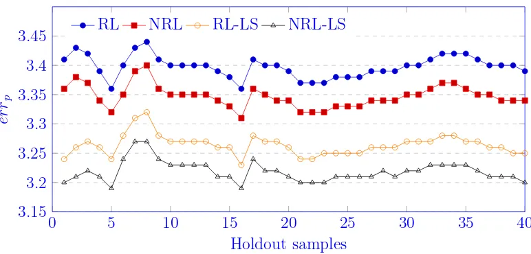
Figure 7: Average of the test error values over holdout samples

parameters is used to compute the test errors erri

erri =−

1

|P Si|

X

σj∈P Si

lnP(σj,βˆi)

where P Si is the size of prediction sample i. Thenerri is a random variable

that depends on the holdout sample i. In order to have unconditional test error values we compute the average of erri values over samples as follows

errp =

1

p

p

X

i=1

erri ∀1≤p≤40. (22)

The values of errp, 1≤p≤ 40 are plotted in Figure 7 and Table 7 reports

the average of the test error values over 40 samples given by the RL, RL-LS, NRL, NRL-LS models. For each model the value of errp becomes more

7

Conclusion

This paper has presented the NRL model which avoids the IIA property of the RL model by allowing scale parameters to be link specific while keeping the advantages of the RL model. We have proposed an efficient approach to estimate the model, solving the value functions using an iterative method with dynamic accuracy. Moreover, we have derived the gradient of the log-likelihood function which can be computed by solving systems of linear equa-tions.

We have provided numerical results using real data. The parameter esti-mates are sensible and the NRL model has significantly better fit than the RL model. The LS attribute plays an important role and the best models in-cluding this attribute have significantly better model fit than those without. We have also provided a cross-validation study suggesting that NRL-LS and NRL are better than the RL-LS and RL model, respectively.

In future research we plan to investigate further the importance of the LS attribute and its definition. Moreover, there are only few attributes available in the data set used in this paper. We would like to test the model on other data sets that allows us to test other possible functional forms of the scale parameters.

In this paper we use a unimodal network and observations of trips made by car. We emphasize that the model is not restricted to this type of network. More precisely, by adapting the state space, the model can be used in e.g. dynamic networks (state is time and location) and multi-modal networks (state is location and mode) as long as link attributes are deterministic. The dynamic network is suitable for modeling congested networks, the RL model has been used for this purpose by Ramos et al. (2012). The challenge lies in the size of the state space, which is considerably larger than a static network since it is the number of links multiplied by the number of time intervals.

As a final remark we note that since the RL and NRL models are based on the universal choice set (including all path even those with loops), they avoid having to consider choice set formation. They can therefore be seen as alternatives to the approach proposed by Manski (1977). The RL and NRL may be relevant to other contexts than route choice where there is an issue associated with large choice sets.

Acknowledgement

Parameters RL NRL RL-LS NRL-LS

b

βT T -2.494 -1.854 -3.060 -2.139

Rob. Std. Err. 0.098 0.132 0.103 0.145

Rob. t-test(0) -25.45 -14.05 - 27.709 -14.75

b

βLT -0.933 -0.679 -1.057 -0.748

Rob. Std. Err. 0.030 0.043 0.029 0.047

Rob. t-test(0) -31.10 -15.79 -36.448 -15.91

b

βLC -0.411 -0.258 -0.353 -0.224

Rob. Std. Err. 0.013 0.016 0.011 0.015

Rob. t-test(0) -31.62 -16.13 -32.091 -14.93

b

βU T -4.459 -3.340 -4.531 -3.301

Rob. Std. Err. 0.114 0.200 0.126 0.207

Rob. t-test(0) -39.11 -16.7 - 35.960 -15.95

b

βLS - - -0.227 -0.155

Rob. Std. Err. - - 0.013 0.013

Rob. t-test(0) - - -17.462 -11.92

b

ωT T - 0.515 - 0.341

Rob. Std. Err. - 0.255 - 0.288

Rob. t-test(0) - 2.02 - 1.18

b

ωLS - -0.674 - -0.581

Rob. Std. Err. - 0.093 - 0.090

Rob. t-test(0) - -7.25 - -6.46

b

ωOL - -0.086 - -0.092

Rob. Std. Err. - 0.015 - 0.016

Rob. t-test(0) - -5.73 - -5.75

LL(βb) -6303.9 -6187.9 -6045.6 -5952.0

Table 5: Estimation results

Models χ2 _p-value

RL & NRL 232 5.11e-50

RL-LS & NRL-LS 187.2 2.46e-40 NRL & NRL-LS 471.8 1.30e-104

Table 6: Likelihood ratio test results

RL NRL RL-LS NRL-LS

3.392 3.336 3.252 3.204

References

Aguirregabiria, V. and Mira, P. Swapping the nested fixed point algorithm: A class of estimators for discrete markov decision models. Econometrica, 70(4):1519–1543, 2002.

Aguirregabiria, V. and Mira, P. Dynamic discrete choice structural models: A survey. Journal of Econometrics, 156(1):38–67, 2010.

Akamatsu, T. Cyclic flows, markov process and stochastic traffic assignment.

Transportation Research Part B, 30(5):369–386, 1996.

Bekhor, S., Ben-Akiva, M., and Ramming, M. Estimating route choice mod-els for large urban networks. 9th World Conference on Transport Research, Seoul, Korea, 2001.

Ben-Akiva, M. and Bierlaire, M. Discrete choice methods and their appli-cations to short-term travel decisions. In Hall, R., editor, Handbook of Transportation Science, pages 5–34. Kluwer, 1999.

Ben-Akiva, M. The structure of travel demand models. PhD thesis, MIT, 1973.

Berndt, E. K., Hall, B. H., Hall, R. E., and Hausman, J. A. Estimation and inference in nonlinear structural models. Annals of Economic and Social Measurement, 3/4:653–665, 1974.

Chu, C. A paired combinatorial logit model for travel demand analysis. In Proceedings of the fifth World Conference on Transportation Research, volume 4, pages 295–309, Ventura, CA, 1989.

Fosgerau, M., Frejinger, E., and Karlstr¨om, A. A link based network route choice model with unrestricted choice set. Transportation Research Part B, 56(1):70–80, 2013.

Frejinger, E., Bierlaire, M., and Ben-Akiva, M. Sampling of alternatives for route choice modeling. Transportation Research Part B, 43(10):984–994, 2009.

Guevara, C. A. and Ben-Akiva, M. E. Sampling of alternatives in logit mixture models. Transportation Research Part B: Methodological, 58(1): 185 – 198, 2013b. ISSN 0191-2615.

Kelley, C. T. Iterative Methods for Linear and Nonlinear Equations. Society for Industrial and Applied Mathematics, 1995.

Lai, X. and Bierlaire, M. Specification of the cross nested logit model with sampling of alternatives for route choice models. Technical report, TRANSP-OR, EPFL, 2014.

Mai, T., Frejinger, E., and Bastin, F. A misspecification test for logit based route choice models. Technical report, CIRRELT - 32, 2014.

Manski, C. F. The structure of random utility models. Theory and decision, 8(3):229–254, 1977.

McFadden, D. Modelling the choice of residential location. In Karlqvist, A., Lundqvist, L., Snickars, F., and Weibull, J., editors, Spatial Interaction Theory and Residential Location, pages 75–96. North-Holland, Amster-dam, 1978.

Nocedal, J. and Wright, S. J. Numerical Optimization. Springer, New York, NY, USA, 2nd edition, 2006.

Prato, C. G. Route choice modeling: past, present and future research di-rections. Journal of Choice Modelling, 2:65–100, 2009.

Ramos, G., Frejinger, E., Daamen, W., and Hoogendoorn, S. Route choice model estimation in dynamic network based on GPS data. InPresented at the 1st European Symposium on Quantitative Methods in Transportation Systems, Lausanne, Switzerland, 2012.

Rust, J. Optimal replacement of GMC bus engines: An empirical model of Harold Zurcher. Econometrica, 55(5):999–1033, 1987.

Rust, J. Maximum likelihood estimation of discrete control processes. SIAM Journal on Control and Optimization, 26(5):1006–1024, 1988.

Train, K. Discrete Choice Methods with Simulation. Cambridge University Press, 2003.