How to Choose the Level of Significance: A Pedagogical Note

Munich Personal RePEc Archive

How to Choose the Level of Significance:

A Pedagogical Note

Kim, Jae

31 August 2015

Online at

https://mpra.ub.uni-muenchen.de/69992/

How to Choose the Level of Significance:

A Pedagogical Note

Jae H. Kim

Department of Economics and Finance La Trobe University, Bundoora, VIC 3086

Australia

Abstract

The level of significance should be chosen with careful consideration of the key factors such as the sample size, power of the test, and expected losses from Type I and II errors. While the conventional levels may still serve as practical benchmarks, they should not be adopted mindlessly and mechanically for every application.

Keywords: Expected Loss, Statistical Significance, Sample Size, Power of the test

1. Introduction

Hypothesis testing is an integral part of statistics from an introductory level to professional

research in many fields of science. The level of significance is a key input into hypothesis

testing. It controls the critical value and power of the test, thus having a consequential impact

on the inferential outcome. It is the probability of rejecting the true null hypothesis,

representing the degree of risk that the researcher is willing to take for Type I error. It is a

convention to set the level at 0.05, while 0.01 and 0.10 levels are also widely used. Thoughtful

students of statistics sometimes ask: “How do we choose the level of significance?” or “Can

we always choose 0.05 under all circumstances?” Unfortunately, statistics textbooks do not

usually provide in-depth answers to this fundamental question.

 _{Tel: +613 94796616; Email address: J.Kim@latrobe.edu.au}

Students should be reminded that setting the level at 0.05 (0.01 or 0.10) is only a convention,

based on R. A. Fisher’s argument that one in twenty chance represents an unusual sampling

occurrence (Moore and McCabe, 1993, p.473). However, there is no scientific basis for this

choice (Lehmann and Romano, 2005, p.57). In fact, a few important factors must be carefully

considered when setting the level of significance. For example, the level of significance should

be set as a decreasing function of sample size (Leamer, 1978; Degroot and Schervish, 2012;

Section 9.9), and with a full consideration of the implications of Type I and Type II errors (see,

for example, Skipper et al., 19671). Although a good deal of academic research has been done

on this issue for many years, these studies are not readily accessible to the students and teachers

of basic statistics. In this paper, I present several examples that I use in my business statistics

class at an introductory university level. To improve the readability, the references for

academic research are given in a separate section.

2. Sample size (Power and Probability of Type II error)

Let  represent the level of significance which is the probability of rejecting the true null

hypothesis (Type I error); and β the probability of accepting the false null hypothesis (Type II

error), while 1- β is the power of the test. For simplicity, we assume that the expected losses

from Type I and II errors are identical, or the researcher is indifferent to the consequences of

these errors. This assumption will be relaxed in the next section. Under this assumption, it is

reasonable to set the level of significance as a decreasing function of sample size, as the

following example shows.

Suppose (X1,…,Xn) is a random sample from a normal distribution with the population mean 

and known standard deviation of 2. We test for H0:  = 0 against H1:  > 0. The test statistic is

X n n

X

Z 0.5

/

2 

 , where Xis the sample mean. At the 5% level of significance, H0 is

rejected if Z is greater than the critical value of 1.645 or Xis greater than2(1.645)/ n. Note

that the Z statistic is an increasing function of sample size or the critical value for X is a

decreasing function of sample size. This means that when the level of significance is fixed, the

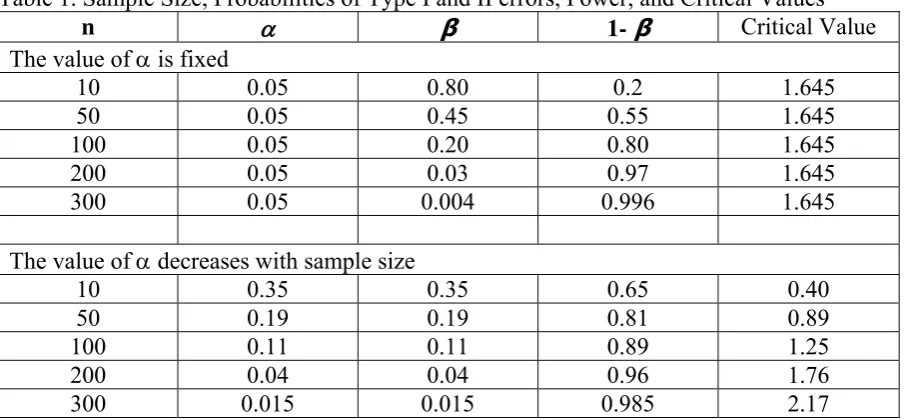
null hypothesis is more likely to be rejected as the sample size increases. Let µ = 0.5 be the

minimum value of substantive importance under H1. Table 1 presents β = P(Z < 1.645|  =

0.5,=2), along with the power and critical values for a range of sample sizes. The upper panel

presents the case where  is fixed at 0.05 for all sample sizes, while the lower panel presents

the case where  is set as a decreasing function of sample size and in balance with the value of

β. The upper panel shows that, when the sample size is small, the value of β is unreasonably

high compared to  = 0.05, resulting in a low power of the test. When the sample size is large,

the power of the test is high, but it appears that  is unreasonably high compared to β. For

example, when the sample size is 300,  = 0.05 is 12.5 times higher than the value of β. In this

case, a negligible deviation from the null hypothesis may appear to be statistically significant

(see Figure 1 and the related discussion).

From the lower panel, we can see that, by achieving a balance between the probabilities of

committing Type I and II errors, the test enjoys a substantially higher power for nearly all cases.

For example, when the sample size is 10 with  = 0.05, the power of the test is only 0.20.

However, if  is set at 0.35, the power of the test is 0.65. When n = 300, setting  = 0.015

provides a balance with the value of β. In addition, the sum of the probabilities of Type I and

can be achieved when  is set as a decreasing function of sample size and in balance with the

value of β (see also Figure 3 and the related discussion).

Figure 1 presents two scatter plots (labelled A and B) between random variables Y and X, both

with sample size 1000. The two plots are almost identical, showing no linear association

between the two. In fact, Y and X are independent in Plot A; but in Plot B, they are related with

the correlation of 0.05. Regressing Y on X in Plot A, the slope coefficient is 0.04 with t-statistic

1.23 and p-value 0.22, indicating no statistical significance at any reasonable level. In Plot B,

the regression slope coefficient is 0.09 with t-statistic 2.82 and p-value 0.004. In this case,

although X and Y are related with a negligible correlation, the regression slope coefficient is

statistically significant at 1% level of significance. Figure 2 plots two scatter plots (labelled A

and B) when the sample size is small. In Plot A, Y and X are independent; but in Plot B, they

are related with a substantial correlation of 0.50 with a clear positive relationship. In Plot A,

the estimated slope coefficient is small and statistically insignificant, as might be expected; but

in Plot B, the estimated slope coefficient (0.42) is large but statistically insignificant (t-statistic

= 1.49 and p-value = 0.23). In this case, although X and Y are related with a relatively high

linear association, the slope coefficient is statistically insignificant at any conventional level of

significance.

The two examples in Figures 1 and 2 illustrate that the t-statistic and p-value can give a wrong

impression or illusion about the true nature of the relationship (see further discussion in Section

4 with reference to Soyer and Hogarth; 2012). In the example given in Figure 1, considering

the large sample size, a much lower level of significance (such as 0.005 or 0.001) should be

adopted, which will deliver the decision of a marginal or no statistical significance (see further

considering the low power, the level of significance should be set at a much higher level such

as 0.30 (see Kim and Choi, 2016)

3. Expected losses from Type I and II errors

Students should be reminded that Type I and II errors often incur losses which affect people’s

lives, such as ill health, false imprisonment, and economic recession (see, for example, Ziliak

and McCloskey, 2008). The level of significance should be chosen taking full account of these

losses. Setting  to a conventional level for every application may mean that the researcher

does not explicitly consider the consequences or losses resulting from Type I and II errors in

their decision-making.

Example: Testing for No Pregnancy

Consider a patient seeing a doctor to check if she is pregnant or not. The doctor maintains the

belief that the patient is not pregnant until a medical test provides the evidence otherwise. The

doctor is testing for the null hypothesis that the patient is not pregnant against the alternative

that she is. Suppose two tests for pregnancy are available: Tests A and B. Test A has a 5%

chance of showing evidence for pregnancy when the patient is not in fact pregnant (Type I

error); but it has a 20% chance of indicating evidence for no pregnancy when in fact the patient

is pregnant (Type II error). Test B has a 20% chance of Type I error and a 5% chance of Type

II error. The consequence of Type I error is diagnosing a patient as pregnant when in fact she

is not; while that of Type II error is that the patient is told that she is not pregnant when in fact

she is. Test A has four times smaller chance of making the Type I error; but it has four times

more chance of making the Type II error. If the doctor believes that Type II error has more

serious consequences than Type I error since the former risks the lives of the patient and baby,

Example: Hypothesis Testing as a Legal Trial

Hypothesis testing is often likened with a trial where the defendant is assumed to be innocent

(H0) until the evidence showing otherwise is presented. The jury returns a guilty verdict when

they are convinced by the evidence presented. If the evidence is not sufficiently compelling,

then they deliver a “not guilty” verdict. In the court of law, there are different standards of

evidence that should be presented, as Table 2 shows. For a civil trial, a low burden of proof

(preponderance of evidence) is required since the consequences of wrong decisions are not

severe. However, for a criminal trial where the final outcome may be the death penalty or

imprisonment, a tall bar (beyond reasonable doubt) is required to reject the null hypothesis.

This means that the legal system is using different levels of significance (or critical values)

depending on the consequences of wrong decisions. That is, the level of significance for

“preponderance of evidence” may be as high as 0.40; and that for “clear and convincing

evidence” can be as low as 0.01. To meet the level of “beyond reasonable doubt”, the level of

significance should be much lower (say 0.0001) which places a tall bar for a guilty verdict.

Example: Minimizing Expected Losses

Consider a business analyst testing for the null hypothesis that a project is not profitable against

the alternative that it is. Suppose for the sake of simplicity that P(H0 is true) = P(H1 is true) =

0.5. Let L1 and L2 be the losses from Type I error and Type II error, then the expected loss from

wrong decisions is 0.5L1 + 0.5βL2. Table 3 presents these values using two different scenarios

of (L1, L2). In the first scenario, the loss from Type II error is five times higher than that of

Type I error, i.e., (L1, L2) = (20, 100); and the opposite is the case for the second scenario.

When the analyst chooses  of 0.05, the corresponding value of β is assumed to be 0.25; and

Suppose the analyst wishes to minimize the expected loss. Then, when (L1, L2) = (20, 100), (,

β) = (0.25, 0.05) should be chosen since it is associated with a lower expected loss. Since the

loss from Type II error is substantially higher, a higher  level should be chosen so that a lower

probability is assigned to Type II error. Similarly, under (L1, L2) = (100, 20), (, β) = (0.05,

0.25) should be chosen. This illustrative example demonstrates that when the losses from Type

I and II errors are different, the level of significance should be set in consideration of their

relative losses.

4. Summary of Selected Academic Research

Leamer (1978; Chapter 4) makes the most notable academic contribution to this issue by

presenting a detailed analysis as to how the level of significance should be chosen in

consideration of sample size and expected losses2. He introduces the line of enlightened

judgement, which is obtained by plotting all possible combinations of (, β) given the sample

size. In the context of the example in Table 1, the line of enlightened judgement is all possible

combinations of (i, β_i) where _i P(Z CR_i|0.5, 2) and CRi is the critical value

corresponding to i. Leamer (1978) shows how the optimal level of significance can be chosen

by minimizing the expected losses from Type I and II errors, and demonstrates that the optimal

significance level is a function of sample size and expected losses.

Figure 3 presents three lines of judgement corresponding to the (, β) values in Table 1 when

the sample size is 10, 50, and 100. Given the sample size, the line depicts a trade-off between

2 _{Note that Manderscheid (1965) and DeGroot (1975, p.380) also propose the same method for choosing the}

 and β. As the sample size increases, the line shifts towards the origin as the power increases.

The green line represents the case where the level of significance is fixed at 0.05. The (, β)

values in the upper panel of Table 1 correspond to the points where this line and the lines of

enlightened judgement intersect. The 45-degree line connects the points where the value of

+ is minimized for each line of enlightened judgement (assuming L1=L2), which correspond

to the (, β) values in the lower panel of Table 1. Kim and Ji (2015) also discuss the line of

enlightened judgement with an example in finance.

Based on the line of enlightened judgement, Kim and Choi (2016) obtain the optimal level of

significance for a range of popular unit root tests and report that the optimal levels of unit root

testing are in the 0.20 to 0.40 range. Fomby and Guilkey (1978) show, through extensive Monte

Carlo simulations, that the optimal level of significance for the Durbin-Watson test should be

around 0.5, much higher than the conventional levels. These results are consistent with the

conjectures made by earlier authors. Kish (1959)3

states that when the power is low, the level

of significance much higher than the conventional levels may be more appropriate. Winer

(1962) also states that “when the power of the tests is likely to be low …, and when Type I and

Type II errors are of approximately equal importance, the 0.3 and 0.2 levels of significance

may be more appropriate than the .05 and .01 levels” (cited in Skipper et al., 1967)4

.

Keuzenkamp and Magnus (1995, p.20) conduct a survey of economics papers and report that

“the choice of significance levels seems arbitrary and depends more on convention and,

occasionally, on the desire of an investigator to reject or accept a hypothesis”. They also note

that Fisher’s theory of significance testing is intended for small samples, stating that “Fisher

does not discuss what the appropriate significance levels are for large samples”. Labovitz

(1968)5

argues that sample size is one of the key factors for selecting the level of significance,

along with the power or probability of Type II error (β) of the test. Ziliak and McCloskey (2008,

p.8) state that “without a loss function, a test of statistical significance is meaningless”, arguing

that hypothesis testing without considering the potential losses is not ethically and

economically defensible. Kish (1959)6 asserts that (at the conventional level of significance)

“in small samples, significant, that is, meaningful, results may fail to appear statistically

significant. But if the sample size is large enough, the most insignificant relationships will

appear statistically significant”. From a recent survey of papers published in finance journals,

Kim and Ji (2015) report that the conventional levels of significance are almost exclusively

used in finance research, despite the widespread use of large or massive sample size.

Gigerenzer (2004, p.601) argues that “the combination of large sample size and low p-value is

of little value in itself”. Engsted (2009, p.401) points out that using the conventional level

“mechanically and thoughtlessly in each and every application” is meaningless.

From a survey of academic economists, Soyer and Hogarth (2012) find that regression statistics

can create an illusion of strong association. They find that the surveyed economists provide

better predictions when they are presented with a simple visual representation of the data than

when they are confronted only with regression statistics (as in Figures 1 and 2). By reconciling

the classical and Bayesian methods of significance testing for a large number of the papers

published in psychology journals, Johnson (2013) finds that p-values of 0.005 and 0.001

correspond to strong and very strong evidence against H0, while the p-values in the

neighbourhood of 0.05 and 0.01 reflect only modest evidence. Based on this, Johnson (2013)

recommends adoption of the “revised standards for statistical evidence” by setting the level of

significance at 0.005 or 0.001, instead of 0.05 and 0.01 (as in the example in Figure 1).

6. Concluding Remarks

Although the level of significance is an important input to hypothesis testing, modern statistical

textbooks allocate surprisingly little space on the discussion as to how it should be chosen for

sound statistical inference. This paper presents such a discussion with several examples for

students, along with the selected references to the past and recent academic research. While the

conventional levels may still serve as useful benchmarks, mindless and mechanical choice of

these levels should be avoided. Students of basic statistics should understand that the level of

significance should be chosen with relevant contexts in mind, in careful consideration of the

key factors such as sample size and expected losses. Recently, the American Statistical

Association warns that "Widespread use of 'statistical significance’ (generally interpreted as 'p

< 0.05') as a license for making a claim of a scientific finding (or implied truth) leads to

considerable distortion of the scientific process (Wasserstein and Lazar, 2016). The level of

significance determines the threshold of statistical significance, and it should be set with care

References

DeGroot, M. 1975. Probability and Statistics, 2nd ed. Reading, MA: Addison-Wesley.

DeGroot, M. H. and Schervish, M. J., 2012, Probability and Statistics, 4th _edition,

Addison-Wesley, Boston

Engsted, T. 2009, Statistical vs. economic significance in economics and econometrics: Further comments on McCloskey and Ziliak, Journal of Economic Methodology, 16, 4, 393-408.

Fomby, T. B. Guilkey, D. K., 1978, On Choosing the Optimal Level of Significance for the Durbin-Watson test and the Bayesian alternative, Journal of Econometrics, 8, 203-213.

Gigerenzer, G. 2004, Mindless statistics: Comment on “Size Matters”, Journal of Socio-Economics, 33, 587-606.

Johnson, V. E. 2013, Revised standards for statistical evidence, Proceedings of the National Academy of Sciences, www.pnas.org/cgi/doi/10.1073/pnas.1313476110

Keuzenkamp, H.A. and Magnus, J. 1995, On tests and significance in econometrics, Journal of Econometrics, 67, 1, 103–128.

Kim, J. H. and Ji, P. 2015, Significance Testing in Empirical Finance: A Critical Review and Assessment, Journal of Empirical Finance 34, 1-14.

Kim, J. H. and Choi, I. 2016, Unit Roots in Economic and Financial Time Series: A Re-Evaluation at the Optimal Level of Significance:

http://papers.ssrn.com/sol3/papers.cfm?abstract_id=2700659

Kish, L. 1959, Some statistical problems in research design, American Sociological Review, 24, 328-338.

Labovitz, S. 1968, Criteria for selecting a significance level: a note on the sacredness of 0.05, The American Sociologist, 3, 200-222.

Leamer, E. 1978, Specification Searches: Ad Hoc Inference with Nonexperimental Data, Wiley, New York.

Lehmann E.L. and Romano, J.S. 2005, Testing Statistical Hypothesis, 3rd _{edition, Springer,}

New York.

Manderscheid, L.V., 1965, Significance Levels-0.05, 0.01, or ?, Journal of Farm Economics, 47 (5), 1381-1385.

Moore, D.S. and McCabe, G.P. 1993, Introduction to the Practice of Statistics, 2nd _edition,

Morrison, D. E. and Henkel, R. E. 1970, The Significance Test Controversy: A Reader, edited by D. E. Morrison and R. E. Henkel. Aldine Transactions, New Brunswick, NJ.

Skipper, J. K. JR., Guenther, A. L. and Nass, G. 1967, The sacredness of .05: a note on concerning the use of statistical levels of significance in social science, The American Sociologist, 2, 16-18.

Soyer, E. and Hogarth, R. M. 2012, The illusion of predictability: How regression statistics mislead experts, International Journal of Forecasting, 28, 695-711.

Wasserstein R. L., Lazar, N. A. 2016, The ASA's statement on p-values: context, process, and purpose, The American Statistician, DOI: 10.1080/00031305.2016.1154108

Winer, B. J. 1962, Statistical Principles in Experimental Design, New York, McGraw-Hill.

Table 1. Sample Size, Probabilities of Type I and II errors, Power, and Critical Values

n  β 1-β Critical Value

The value of  is fixed

10 0.05 0.80 0.2 1.645

50 0.05 0.45 0.55 1.645

100 0.05 0.20 0.80 1.645 200 0.05 0.03 0.97 1.645

300 0.05 0.004 0.996 1.645

The value of  decreases with sample size

10 0.35 0.35 0.65 0.40 50 0.19 0.19 0.81 0.89 100 0.11 0.11 0.89 1.25 200 0.04 0.04 0.96 1.76 300 0.015 0.015 0.985 2.17

n: sample size; : the level of significance; : Probability of Type II error, 1-: power of the test

Table 2. Burden of Proof in Legal Trials

Burden of Proof Description Trials Preponderance of

Evidence

Greater than 50% chance

Civil, Family: Child support, unemployment benefit Clear and Convincing Evidence Highly and substantially probable

Civil, Criminal: Paternity, Juvenile delinquency, Probate, Decision to remove

life support Beyond Reasonable

Doubt

No plausible reason to believe otherwise

Criminal: Imprisonment, Death Penalty

Table 3. Expected Losses from Hypothesis Testing

(L1, L2) = (20, 100) (L1, L2) = (100, 20)

(, β) = (0.05, 0.25) 13 5

(, β) = (0.25, 0.05) 5 13

Figure 1. Statistical Significance and Sample Size (A case of Large Sample)

X ~ N(0,1) and Y ~ N(0,1) with sample size 1000.

Plot A: Y and X independent; and the regression slope coefficient is statistical insignificant.

Plot B: Y and X are related with negligible correlation of 0.05, but the regression slope coefficient is statistically significant at the 1% level.

The same random numbers are used for both plots.

-3 -2 -1 0 1 2 3

-3

-2

-1

0

1

2

3

PLOT A

X

Y

-3 -2 -1 0 1 2 3

-3

-2

-1

0

1

2

3

PLOT B

X

Figure 2. Statistical Significance and Sample Size (A case of Small Sample)

X ~ N(0,1) and Y ~ N(0,1) with sample size 5.

Plot A: Y and X independent; and the regression slope coefficient is statistical insignificant.

Plot B: Y and X are related with negligible correlation of 0.50, but the regression slope coefficient is statistically insignificant at the 10% level.

The same random numbers are used for both plots.

-1.5 -1.0 -0.5 0.0 0.5

-0

.4

-0

.2

0

.0

0

.2

0

.4

0

.6

PLOT A

X

Y

-1.5 -1.0 -0.5 0.0 0.5

-0

.5

0

.0

0

.5

PLOT B

X

Figure 3. Examples of the Line of Enlightened Judgement

The horizontal line corresponds to  = 0.05.

The 45-degree line corresponds to the points where + is minimized (assuming L1=L2).

0.0 0.2 0.4 0.6 0.8 1.0

0.

0

0

.2

0.

4

0.

6

0.

8

1.

0

beta=Prob(Type II Error)

al

ph

a=

P

rob

(T

y

p

e I

E

rr

or

)

n=10

n=50