Forecasting Nigerian Inflation using Model Averaging methods: Modelling Frameworks to Central Banks

Munich Personal RePEc Archive

Forecasting Nigerian Inflation using

Model Averaging methods: Modelling

Frameworks to Central Banks

Tumala, Mohammed M and Olubusoye, Olusanya E and

Yaaba, Baba N and Yaya, OlaOluwa S and Akanbi, Olawale

B

Department of Statistics, Central Bank of Nigeria, Department of

Statistics, University of Ibadan, Nigeria, Department of Statistics,

Central Bank of Nigeria, Department of Statistics, University of

Ibadan, Nigeria, Department of Statistics, University of Ibadan,

Nigeria

December 2017

Online at

https://mpra.ub.uni-muenchen.de/88754/

Forecasting Nigerian Inflation using Model Averaging methods:

Modelling Frameworks to Central Banks

M.M. Tumala1 _{O.E. Olubusoye}2 _{B.N. Yaaba}1 _{O.S. Yaya}2 _{O.B. Akanbi}2

1_{Department of Statistics, Central Bank of Nigeria}

2_{Department of Statistics, University of Ibadan, Nigeria}

As a result of the adverse macroeconomic effect of inflation on welfare, fiscal budgeting, trade performance, international competitiveness and the whole economy, inflation still remains a subject of utmost concern and interest to policy makers. The traditional Philips curve as well as other methodologies have been criticized for their inability to track correctly the pattern of inflation, particularly, these models do not allow for enough variables to be included as part of the regressors, and judgment is often made by a single model. In this work, model averaging techniques via Bayesian and frequentist approach were considered. Specifically, we considered the Bayesian model averaging (BMA) and Frequentist model averaging (FMA) techniques to model and forecast future path of CPI inflation in Nigeria using a wide range of variables. The results indicated that both in-sample and out-of-sample forecasts were highly reliable, judging from the various forecast performance criteria. Various policy scenarios conducted were highly fascinating both from the theoretical perspective and the prevailing economic situation in the country.

Key words: Bayesian model averaging; Forecasting; Frequentist approach; Inflation rate; Nigeria

1. Introduction

The need to ensure an effective conduct of monetary policy by the central bank has made

inflation forecasting very essential. Due to the traditional argument of lags in the monetary

policy transmission mechanism, inflation forecast therefore plays a crucial role in the conduct

of monetary policy. There are long lags between monetary policy actions and their impact on

the economy. Policies responding only to the current state of the economy may not prove to be

good stabilizers, therefore, it is generally recognized that central bank policies must be

far-sighted.

1 _{This is part 2 of the abridged version of the full report on Forecasting and Determining the Predictors of Inflation}

There is no gainsaying the fact that a lot of progress and development has been made

in terms of both theoretical and econometric modelling in the recent times, and forecasting

inflation remains an arduous task requiring more attention and efforts. With the rapid changes

in the Nigerian economy often caused by different shocks, the task of forecasting inflation has

become even more difficult. The ambiguous and changing structure of the Nigerian economy

further complicates this task. However, producing a real-time macroeconomic forecasting

particularly, in a developing economy like Nigeria is such a complex and challenging problem.

In advanced economies, forecasting process often employs a variety of formal models, which

include structural and purely statistical. The forecasts of inflation are usually developed

through an eclectic process that combines model-based projections, anecdotal and other “extra

model” information as well as professional judgement.

The most common tool for inflation forecasting is probably the Phillips curve which

uses a single measure of economic slack such as unemployment to predict future inflation. The

Phillips curve equation uses the rate of unemployment or some other aggregate economic

measures in predicting inflation rate. Some recent specifications of Phillips curve equations

relate the current rate of unemployment to future changes in inflation rate. The main idea

behind this specification is that there is a baseline rate of unemployment at which inflation

tends to remain constant. There is, the popular feeling that inflation tends to rise over time

when unemployment is below this baseline rate, and inflation falls when unemployment is

above this baseline rate. The term non-accelerating inflation rate of unemployment (NAIRU)

is used to describe this baseline unemployment rate. Hence, modern specifications based on it

are referred to as NAIRU Phillips curves.

The NAIRU Phillips curves have become so popular in academic literature on inflation

forecasting, and among policy making institutions, because of the view that inflation forecasts

argues that “the empirical Phillips curve has worked amazingly well for a decade” and then

concludes based on this empirical success that a Phillips curve should have “a prominent place

in the core model” used for macroeconomic policy making purposes. The literature on studies

based on the extension of Phillips curve is rather too voluminous but a few representative and

prominent ones include Stock and Watson (1999), Ang et al. (2007), Stock and Watson (2008)

and Groen et al. (2009).

However, the usefulness of Phillips curve for predicting inflation has been challenged

and questioned by many authors. For instance, Atkeson and Ohanian (2001) obtained a

short-run variant of the curve by regressing the quarterly change in the rate of inflation on the

unemployment rate with a constant. The study shows that the short-run Phillips curve does not

represent a stable empirical relationship that can be exploited for constructing a reliable

inflation forecasts.

T

slope of the short-run Phillips curve) varies significantly across different sample periods.

Substantial progress has been made by researchers in the aspect of using many

predictors in forecasting inflation. Information in these large variables is combined in a sensible

manner to prevent the estimation of a large number of unrestricted parameters. Stock and

Watson (2001, 2002) submit that the best predictive performance is obtained by averaging

forecasts constructed from several models. This popular approach is referred to in the literature

as the Bayesian Model Averaging (BMA), initiated by Leamer (1978). BMA efficiently and

systematically evaluates a wide range of predictor variables for inflation and (almost) all

possible models that these predictors in combination can give rise to. Using the posterior

probabilities of the models, weights are assigned to the different models to obtain a weighted

model averaging.

In the present paper, the burning research questions is: How does a single model

overarching objective of this paper is to analyse a wide spectrum of CPI inflation predictors

and all possible models that can arise from combining the models using Bayesian Model

Averaging. Specifically, the study objectives to be pursued are to: (1) analyse and forecasts

from all the models combining predictors of price inflation based on BMA approach; and, (3)

make policy scenarios based on the BMA forecasts.

The structure of the paper is as follows: Section 1 introduces the work. Section 2

reviews available literature on inflation modelling by apex banks, African banks, international

monetary organizations, the Central Bank of Nigeria and individual researchers. Section 3

presents methodology on model averaging techniques, that is, the FMA and BMA. Section 4

presents the data, empirical results as well as some policy scenarios. Section 5 gives the

summary, conclusion and renders policy implications.

2. Review of Literature

Various inflation forecasting models have been applied in forecasting inflation rates in apex

banks of developed and developing countries. In Bank of Japan, Fujiwara and Koga (2002)

presented a statistical forecasting method (SFM) that related many economic and financial time

series data without making structural assumptions other than setting up the underlying

variables. The SFM was built on many VAR models from combinations of the underlying

variables. The data considered were the CPI, domestic wholesale price index, import price,

industrial production index, investment, unemployment rate, monetary aggregate, government

bond yield and effective exchange rate. The result showed that SFM could provide reliable

forecasts information that cannot be extracted when a single structural-type estimating is used.

Bruneau et al. (2003) assessed the usefulness of dynamic factor models of Bank of

France for generating headline and harmonized index of consumer prices (HICP) inflation

methodology and estimated within the sample period 1988:01 and 2002:03 for inflation, with

balanced and unbalanced panels. The total HICP, as well as its five main sub-components

(manufacturing, services, processed food, unprocessed food and energy were used across the

Euro countries. Their results showed evidence to support the improvement of factor/or

combined factors in modelling than using the simple AR model for forecasting HICP core

inflation and total inflation, and the overall results were found to be robust to potential

data-snooping.

Since 2011, the Bank of England inflation forecasting platform developed a Central

Organizing Model for Projection Analysis and Scenario (COMPASS). The model was

designed to organize framework for predicting inflation. The model is a New Keynesian,

Dynamic Stochastic General Equilibrium (DSGE) model estimated using Bayesian methods.

From the onset, before the inception of Monetary Policy (MPC), the bank focused on both GDP

and inflation (Bank of England, 2015), while MPC introduced other nine variables. Altogether,

the Bank of England considered, in modelling and forecasting inflation, variables such as the

real GDP, inflation, the unemployment rate, real private consumption, real total investment,

nominal wages, nominal house prices, nominal household lending, nominal corporate lending,

US real GDP and euro-area real GDP. The accuracy of Bank forecasts were then compared to

forecasts from simple model, and for a subset of those eleven variables. The forecasts accuracy

was also compared with UK private sector forecasters and other central banks, and the results

indicated that Bank forecasts based on COMPASS resulted in smallest forecasts error as

compared to other forecasts from other private sectors and other central banks (Bank of

England, 2015).

In South African Reserve Bank, Fedderke and Liu (2016) considered the relative

performance of models for forecasting inflation. These models included the classical Phillips

inflation included excess demand, unit labour cost, nominal wage rate, real labour productivity,

exchange rate, real wage, supply-side shock, money balances, government expenditure and

government surplus/deficit. By decomposing unit labour cost into changes in the nominal wage

and real labour productivity, the authors found a strong positive association between inflation

and nominal wages, while they observed weak negative association between real labour

productivity and inflation. On the long run, supply side shocks revealed significant association

with inflation, while as to demand side shocks, the output gap does not return a robust statistical

association with inflation but growth in the money supply and government expenditure

indicated consistent association with inflationary pressure.

Gaomab (1998) reviewed inflation dynamics for Namibian Bank for the past 24 years

using data spanning between 1972 and 1996. The model applied cointegration technique and

ECM, both with structural stability tests in making time series forecasts. The variables

considered were the CPI, real GDP, broad money supply, nominal interest rate, US dollar ex

change rate, South African CPI and US CPI. The results showed dominant influence of South

African macroeconomy on Namibian inflation. On the long run, US economy, representing the

influence of the rest of the world, also has considerable influence on Namibian prices.

Waiquamdee (2001) presented a Bank of Thailand Macroeconomic Model (BOTMM)

which is a system of equations representing transmission mechanisms in the economy and the

relationships among economic variables. This model gives information on the prospects for

growth and inflationary trend and assists in monetary policy decisions. The BOTMM system

incorporates a total of 17 equations with ECM properties. These are equations on consumption,

private investment, volume of export and import, energy price, domestic retail oil price, public

investment deflator, government consumption deflator, and export and import prices. The

results, except with the limitation that it allows for short-period of observations and the

coefficients in some equations are not stable.

Gonzalez et al. (2006) developed a short-run food inflation model to predict inflation

in Colombia. The model disaggregated food items based on economic theory and employed

least squares method with structural breaks in its specification. The results obtained indicated

significant improvement of the model when food items were disaggregated into processed

foods, unprocessed foods and food away from home. The findings further suggested the

importance of combining forecasts from alternative models.

Bjornland et al. (2009) developed a system for generating model-based forecasts for

Norwegian inflation rates by using a set of five models: the ARIMA, vector autoregressive

(VAR), Bayesian VAR (BVAR), error correction models (ECM), factor model and dynamic

stochastic general equilibrium (DSGE) models with each model having several model variants,

resulting in a total of 80 model combinations. The variables considered were the GDP, interest

rates, inflation, exchange rate, terms of trade, oil price, consumption growth, investment

growth, export growth, employment rate and real wage growth. The data were sampled

between 1987Q1 to 1998Q4, and forecasts were generated recursively from 1999 to 2008, and

the performance of these models over this period was then used to derive weights that were

used to combine the forecasts. The results showed that model combinations approach improved

upon the point forecasts from individual models and outperformed Norges Banks forecasts for

inflation. Norman and Richards (2010) estimated a range of single-equation models for

Australian inflation. Having considered standard Phillips curve, the New-Keynesian Phillips

Curve (NKPC) and other mark-up model on quarterly headline CPI, output gap, unit of labour

costs growth and import prices, the standard Phillips curve model emerged the best, followed

As reported in Figueiredo (2010), the Central Bank of Brazil applied a Bayesian VAR

model with principal components and other model combinations such as unrestricted VAR,

partial least square methodology (PLS), factor analysis and principal component model in

forecasting inflation in Brazil. The author considered the real interest rate, nominal interest

rate, money stock, industrial output, nominal exchange rate, regulated price and market price.

It was found that the best forecasting model emerged when the forecasts were generated at

6-step ahead. Furthermore, factor model with targeted predictors presented the best forecast

results, while PLS showed relatively poor result. The work further recommended the use of

other rich-data approach such as the Bayesian Model Averaging (BMA) in modelling inflation.

Younus and Roy (2016) applied Unrestricted VAR model in forecasting inflation rates in

Bangladesh. The authors considered data spanning between July 2006 and June 2016. In the

VAR system, real GDP growth rate, money supply (M2), private sector credit, exchange rate,

and world food price index were considered along with the inflation rate. The result of the VAR

model indicated strongest contribution of money supply (M2) and interest rates in predicting

inflation rate.

Giannone et al. (2014) applied Bayesian Vector Autoregressive (BVAR) model to

investigate the interrelationships between main components of the Harmonized CPI and its

determinants and obtained reliable forecasts. Altug and Cakmakli (2015) formulated a

statistical model that combined survey data on inflation expectations with actual inflation data

on Brazil and Turkey. The authors considered the state space model; an autoregressive model;

a backward-looking Phillips curve and a hybrid New Keynesian Phillips Curve. The results

obtained indicated clear alignment of inflation forecasts with survey expectations, that is, the

results showed superiority of predictive power of the proposed framework over the models

In the case of Nigeria, Doguwa and Alade (2013) used four short term inflation

forecasting models for Nigeria within the context of SARIMA and SARIMAX. They utilized

monthly data from July 2001 to September 2013 across fourteen (14) variables sub-divided

into endogenous and exogenous variables. The endogenous variables include consumer price

index, Food consumer price index and core consumer price index. The endogenous variables

comprises of price of petroleum motor spirit per litre, central government expenditure, nominal

Bureau-de-change exchange rate, broad money supply, official nominal exchange rate, reserve

money, net credit to central government, credit to private sector, average monthly rainfall in

cereals producing north central zone and average monthly rainfall in vegetables producing

southern zone. They found parsimonious SARMAX model to be relatively more effective in

predicting inflation. Okafor and Shaibu (2013) adopted a univariate autoregressive integrated

moving average (ARIMA) as suggested by Box and Jenkins (1976) to model and forecast

inflation for Nigeria using CPI data from 1981 to 2010. The result found ARIMA (2,2,3) as the

most adequate for the country as the in-sample forecast and the estimated ARIMA tracked

fairly well the actual inflation for the sampled period. They submitted that inflation expectation

largely drives actual inflation in Nigeria, hence advocated for monetary policy transparency.

Omekara, Ekpenyong and Ekerete (2013) were of the view that inflation in Nigeria is periodic

in nature. They used Periodogram and Fourier series analysis from 2003 to 2011 to model

Nigerian monthly inflation rates. They attributed the periodicity of inflation rate to variations

in government administration. The forecasts generated were found to be accurate for Nigeria.

Using monthly CPI data from 2003 through 2011, Amadi, Gideon and Nnoka (2013)

proposed SARIMA (1,1,0) x (1, 1, 1) to be the most reliable model for monthly inflation rate

of Nigeria. In their study on modelling and forecasting inflation for Nigeria, Otu et al. (2014)

explored ARIMA in line with Box and Jenkins using monthly data covering the period October

November, 2014. They reported ARIMA (1,1,1)(0,0,1) as adequate for Nigeria. The study

attributed the volatility of inflation in Nigeria to money supply, exchange rate depreciation,

petroleum prices and low level of agricultural production.

Kelikume and Salami (2014) adopted a univariate model of the form of Box-Jenkins

model and a multivariate model in the form of vector autoregression to forecast inflation for

Nigeria using monthly data on changes in CPI and broad money supply from January 2003 to

December 2012. The result, according to the authors reported the VAR model as the most

adequate for forecasting inflation in Nigeria because it returned smaller RMSE. Adams et al.

(2014) modelled the Nigerian CPI using ARIMA model in line with Box-Jenkins approach.

They used CPI data between the period 1980 and 2010, and forecast for five years ahead (i.e.

2011 to 2015). The result favoured ARIMA (1, 2, 1) as the most suitable for Nigeria. Yemitan

and Shittu (2015) employed Kalman filter technique to implement a state space model to

forecast inflation for Nigeria using monthly data from January 1995 to December 2014. The

authors introduced structural breaks to capture major political, monetary and macroeconomic

events in the country. They concluded that Kalman filter technique is relatively more efficient

than Box-Jenkins. They attributed the efficiency of Kalman filtration to availability of built-in

which allows information update.

To test the efficacy of artificial neural networks (ANN) in inflation forecasting,

Onimode et al. (2015) applied ANN and AR (1) on Nigeria monthly CPI data from November

2011 to October 2012 and submitted that neural network is more efficient than univariate

autoregressive models in forecasting inflation up to four quarters ahead. Duncan and

Martinez-Garcia (2015) using seasonally adjusted quarterly data on CPI from 1980Q1 to 2016Q4 of

fourteen (14) Emerging Market Economies (EMEs) including Nigeria, adopted both

Frequentist and Bayesian techniques to forecast inflation for Nigeria. The variable considered

production index. The findings support the adequacy of Random Walk based on Atkeson and

Ohanian (RW-AO) as it produces the lowest RMSPEs. The authors therefore suggested that

RW-AO should be used by the EMEs for inflation forecasting.

Employing a Univariate Autoregressive Integrated Moving Average (ARIMA)

modelling in line with Box-Jenkins technique, Kuhe and Egemba (2016) forecasted inflation

for Nigeria using annual CPI data from 1950 to 2014. They found ARIMA (3, 1, 0) to be the

best fit for Nigerian CPI data. The out-of-sample forecast (i.e. 2015 to 2020) reveals a

continuous rise in inflation throughout the period. In a comparative study to determine the more

efficient model between ARIMA-Fourier and Wavelet models, Iwok and Udoh (2016) who

obtained ARIMA-Fourier model by combining both the linear and sinusoidal components of

the CPI utilized MSE, MAE, and MAPE of the two models to determine their adequacy and

concluded that Wavelet model outperformed the ARIMA-Fourier model. They attributed the

performance of Wavelet model to its flexibility in handling non-stationary data as well as the

possibility of simultaneous utilization of information in both time-domain and the frequency

domain. John and Patrick (2016) forecasted monthly inflation rate for Nigeria using data from

January 2000 to June 2015 and found ARIMA (0,1,0) x (0,1,1) to be adequate because the

in-sample forecast obtained was tightly close to the original series. Similarly, Chinonso and

Justice (2016) applied Box-Jenkins ARIMA model on monthly urban and rural CPI from

January 2001 to December 2015 to provide 29 months ahead inflation forecast for Nigeria. The

study selected ARIMA (0,1,0), ARIMA (0,1,13) as the most suitable for forecasting inflation

for Nigeria. By applying the VAR model, Inam (2017) determined and forecasted future path

of inflation rate for Nigeria. The study utilized data on inflation rate, money supply, fiscal

deficit, real exchange rate, interest rate, changes in import prices and real output over the period

1970 to 2012. The result conclude that immediate lag value of inflation largely fuels current

3. Methodology

3.1 Frequentist Model Averaging Technique

A sizable number of frequentist methods for model averaging have been developed in the

literature, and a considerable number of them are on model selection methods. They are

generally considered to be hard-threshold averages. The procedure described below follows

the work of Moral-Benito (2015).

Consider the linear model in matrix form given as follows:







 X_A X_B

y (1)

1

where y, X_A and  are T1 vectors of the dependent variable, the explanatory variable of

interest and the random shocks, respectively. X_B is a

T



k

control variables which may or may not be included in the model, and



the parameters to be estimated. There is altogether a total of 2 possible models that can be k

estimated from (4) if we set some of the components of ' 2

1, ,..., )

(  _k

  to be zeros,

assuming that ˆ_M is the estimator of



) ,..., ,

(M₁ M₂ M₂k

M . Generally, in many applied research, the practice is to take the selected

model, and as given, and carry out statistical inference on this single estimate ˆ_M while the

            selected is model th -2 the if , ˆ . . . selected is model second the if , ˆ selected is model first the if , ˆ ˆ 2 2 1 k M M M k     (2)

Alternatively, (2) can be written as,



ˆ _{ }

 (3) where     0therwise , 0 model candidate the if , 1 ~ j M M j

 . The estimator in (3) suffers some major

drawbacks particularly if model uncertainty is present, especially in the selection of the control

variables for instance. Consider the smoothed weights j M

 , consequently therefore, the FMA

estimator becomes:



ˆ _{ }

 (4)

where 0 1, j M 



 . The FMA estimator of



model selection and parameter estimation. The asymptotic properties of the estimator has been

discussed in Hjort and Claeskens (2003) and the asymptotic distribution is detailed in

Claeskens and Hjort (2008). Notwithstanding, inference based on this limiting distribution still

ignores the uncertainty involved in the model selection procedure because its variance is

obtained by averaging the model specific variances. To overcome this challenge, Buckland et

al. (1997) has proposed an alternative method to deal with the problem of misleading inference

takes extra model uncertainty into consideration by incorporating an extra term in the variance

of the FMA estimator.

Another thorny issue with the FMA estimator is the choice of weights. The FMA

estimator depends heavily on the weights selected for estimation. The weights can be fixed as

noted earlier. However, the use of different weights will produce different asymptotic

properties of the corresponding FMA estimators. Three classes of weight choice techniques

have been proposed in the literature and they are well discussed in Moral‐ Benito (2015). The

first is the weight choice based on information criteria which is probably the most commonly

used approach in FMA. The different information criteria are of the form:

l_j 2log(L_j)_j (5)

where L_j is the maximized likelihood function for the j-th model, _j is a penalty term function

of the number of parameters and/or the number of observations of model j. Consequently,

Buckland et al. (1997) proposed the following as model weights:





 k

j

h h

j M

l l

2

1exp( /2)

) 2 / exp(

 (6)

which are normalized to sum to unity.

Claeskens and Hjort (2003) proposed the use of the Focused Information Criterion

(FIC) to select one single best model rather than information criteria such as the AIC and BIC

in some circumstances. Such circumstances include when one model is best for estimating one

parameter and another model is best for another parameter. It follows naturally that FIC can be

employed as an alternative method of constructing FMA model weights. The second weight

choice technique is based on Mallows’ criterion. Mallows (1973) proposed a Ckstatistic for

model selection in linear regression. The C_k is defined as a criterion for selecting amongst k

Ck RSS k N 2k )

(

2  



 (7)

If model (k) is correct then C_kwill tend to be close to or smaller than k. Therefore, a simple

plot of C_k versus k can be used to decide amongst the model. Sequel to this, Hansen (2007)

proposed to select the model weights in least-squares model averaging by minimizing the

Mallows’ criterion in what has now become Mallows Model Averaging (MMA) estimator.

Although the MMA estimator is asymptotically optimal but the optimality fails under

heteroscedasticity. Hansen (2008) considers forecast combination based on MMA. The method

selects weights by minimizing a Mallows criterion. The third weight choice method is based

on cross-validation criterion. The most recent paper on this is Hansen and Racine (2012) which

proposes a Jackknife Model Averaging (JMA) for obtaining appropriate weights for averaging

M models for improved estimation of an unknown conditional mean in the face of non-nested

model uncertainty in heteroscedastic error settings. The JMA estimator selects weights by

minimizing a cross-validation criterion. Unlike the MMA, the JMA is appropriate for more

general linear models, that is, models with random errors with non-constant variances and

where the candidate models can be non-nested.

3.2Bayesian Model Averaging Technique

The use of BMA for forecast combination was first introduced by Min and Zellner (1993). The

usefulness was demonstrated by Wright (2008, 2009). Stock and Watson (1999, 2004, 2005,

2006) have provided detailed empirical evidence demonstrating the gains in forecast accuracy

through forecast combination, and have demonstrated the success of simple averaging (equal

weights) along with BMA. The BMA implementation begins the formulation of all feasible

models and specifying the prior beliefs about the probability that each model is the true one.

After that the posterior probability that each model is the true one is computed. Finally, the

This looks like a shrinkage methodology, but with the shrinkage over the possible models and

not just over the parameters.

In situations where many potential explanatory variables exist, alternative models can

be defined based on the set of explanatory variables they include. In general, if there are k

potential explanatory variables in a study, then 2k _{models are possible. It is obvious that as k}

gets larger, the number of possible models grows larger. Two major problems are usually

confronted. First is how to handle this considerable number of models. The second relates to

prior information about the models. These problems have largely been surmounted by Bayesian

Model Averaging (BMA) as would be examined during this discussion.

Consider a linear regression model with a constant term, 𝛽₀, and k potential

explanatory variables X X₁, ₂,...,X_k:

y ₀ ₁X₁₂X₂.... _kX_k u (8)

From model (8), there are 2k _{different feasible models based on inclusion and exclusion of each}

regressor. If we let 𝑀_𝑗 for 𝑗 = 1, 2, 3, … , 𝑝 denotes the different models under consideration,

and having constructed the model space, the posterior distribution of any coefficient, say 𝛽_𝑟,

given the data D is:

Pr(𝛽_𝑟|𝐷) = ∑_{𝑗:𝛽𝑟∈𝑀𝑗}Pr(𝛽_𝑟|𝑀_𝑗, 𝐷) Pr(𝑀_𝑗|𝐷) (9)

The logic of Bayesian inference requires one to obtain result for every model under

consideration and average them. The weights in the averaging are the posterior model

probabilities, Pr(𝑀_𝑗|𝐷). These weights are the key feature for estimation via the BMA. The

Posterior Model Probability (PMP) is the ratio of its marginal likelihood to the sum of marginal

Pr(𝑀_𝑗|𝐷) =Pr(𝐷|𝑀𝑗) Pr(𝑀𝑗)

Pr(𝐷) =

Pr(𝐷|𝑀_{𝑗) Pr(𝑀}𝑗)

∑2ki=1Pr(𝐷|𝑀_{𝑖) Pr(𝑀}𝑖)

(10)

where the marginal likelihood of the jth model is

Pr(𝐷|𝑀_𝑗) = ∫ Pr(𝐷|𝛽𝑗, 𝑀_𝑗) Pr(𝛽𝑗|𝑀_𝑗) 𝑑𝛽𝑗 (11)

and 𝛽𝑗is the vector of parameters from model 𝑀_𝑗, Pr(𝛽𝑗|𝑀_𝑗) is a prior probability distribution

assigned to the parameters of model 𝑀_𝑗, Pr(𝑀_𝑗) is the probability that 𝑀_𝑗 is the true model

and Pr(𝐷|𝛽𝑗, 𝑀_𝑗) is the likelihood. The posterior mean and standard deviation of 𝛽 =

𝛽𝑗_{(quantity of interest) are then constructed as}

𝐸[ 𝛽|𝐷] = ∑ 𝛽̂ Pr(𝑀2j=1k 𝑗|𝐷) (12)

𝑉[ 𝛽|𝐷] = ∑ (𝑉𝑎𝑟[𝛽|𝐷, 𝑀2_j=1k _𝑗] + 𝛽̂2) Pr(𝑀_𝑗|𝐷) − 𝐸[ 𝛽|𝐷]2 (13)

where 𝛽̂ = 𝐸[ 𝛽|𝐷, 𝑀_𝑗]. Each Model implies a forecast density 𝑓₁… 𝑓_𝑝, where 𝑝 is the last

model. Similarly, each model produces a point forecast. In reality, the true model is unknown,

thus leading to model uncertainty. In such situation, the point forecast density becomes

𝑓∗ _{= ∑ Pr(𝑀} 𝑗|𝐷) 𝑓𝑗 2k

j=1 (14)

This implies that the point forecast in (9) weights each of the 2k forecasts by the posterior

density of the model. Thus, the weights in the averaging are the posterior model probabilities.

In summary, the BMA approach simply involves the following three steps: (a) specifying the

models, (b) specifying the model priors and (c) and specifying parameter priors. The only thing

remaining is just computation once the three steps are accomplished.

Monthly data were used in this study, these spanning January 2002 to June 2017, based on data

availability across the needed variables. Three key measures of inflation are of interest in the

empirical analysis. These are: all items consumer price index (CPI), core CPI (CCPI) and food

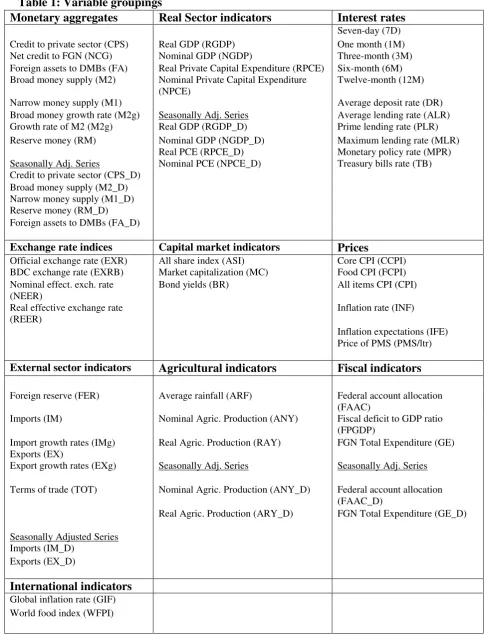
CPI (FCPI). The macroeconomic variables considered in the report are classified into 10 groups

as shown in Table 1.

INSERT TABLE 1 ABOUT HERE

The study adopts a factor-based approach to generate forecasts for each of the three measures

of inflation. This is because of the size of the predictors and the possibility of related variables

providing the same information in explaining the dependent variable. Therefore, principal

component analysis employed in the study is based on the underlying dataset2 _{consisting of 59}

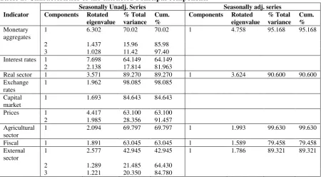
predictors which are classified into 10 groups as shown in Table 1. The principal components

are extracted for each group and used in the BMA model estimation and forecasting. The results

of the principal component analysis are presented in Tables 2 and 3. In Table 2, important

characteristics of the extracted principal components are presented. For the monetary

aggregates containing nine variables, three components were extracted and which accounts for

97.4 percent total variance.3 _{The first component accounts for 70.02 percent of the total}

variance. For the seasonally adjusted monetary aggregates containing five variables, only one

component was extracted which accounts for 95.17 percent total variance. For the interest rate

indicators with 12 variables, two components are extracted. The first component accounts for

64.1 percent of total variance and cumulatively both components account for a total variance

of 81.96 percent. The real sector has four variables. The PCA analysis extracted one component

which accounts for 89.27 percent of the total variance. Exchange rates and capital market, each

2

This total number includes both seasonally adjusted and unadjusted series. Only series having observations from January 2002 to June 2017 are included in the analysis.

3

has one component extracted with total variance of 98.09 percent and 84.64 percent

respectively. The prices category has two extracted components, with the first accounting for

63.10 percent and both cumulatively accounts for 91.46 percent of the total variance. The

agricultural and fiscal categories have one component each with total variance of 69.80 percent

and 63.05 percent respectively. Lastly, for the external sector group, three components are

extracted from the PCA analysis. The first component accounts for up to 42.95 percent and the

three cumulatively accounts for 84.78 percent of the total variance.

INSERT TABLE 2 ABOUT HERE

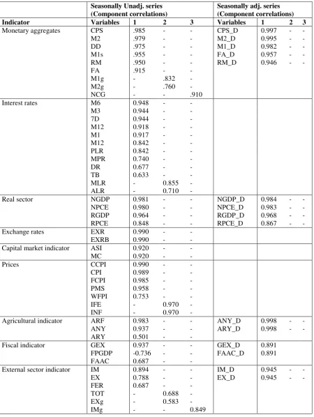
The identified variables in the principal components are presented in Table 3. We present the

results to include up to three components, as in the case of monetary aggregates and external

sector indicators. Generally, the PCA results that are presented in the report agree with the

peculiarity of the Nigerian economy. The first component of the monetary aggregates loads

only six variables. In the seasonally adjusted series, the CPS contributes most follow by the

broad money supply (M2) for both sets of data. For interest rate indicators, six-month interest

time/time deposit rate (M6) loads most with 0.948 correlation as compared to other variants of

interest rate in the principal component. For the real sector indicator, the highest loaded variable

is the nominal gross domestic product (NGDP) for both sets of data. In the case of prices, the

core consumer price index (CCPI) loads most with 0.99 correlation follow by all items CPI

with 0.98 correlation. The rest of the results are presented in Table 3. In all, 18 PCAs, each

representing an index for their respective category, are used as predictor variables in the BMA

model estimation and forecasting.

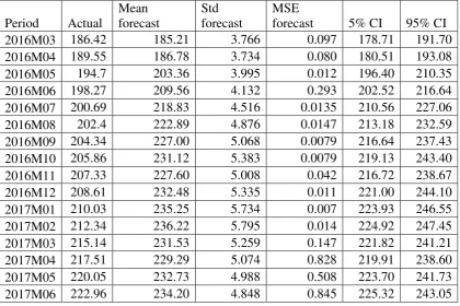
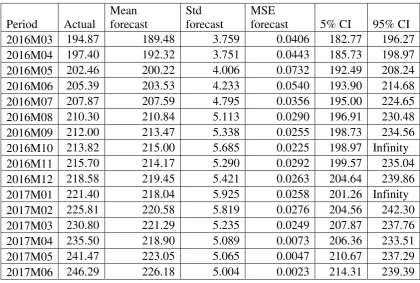
4.2 Model Forecast Performance

The forecast performance of the BMA model is evaluated using the forecast standard error (std

forecast) and the mean square error (MSE). The sample data is divided into two, namely,

training sample (January 2002 to February 2016) and testing sample (March 2016 to June

2017). The Tables 4 to 6 present the results for the testing sample for all items consumer price

index (CPI), core consumer price index (CCPI) and food consumer price index (FCPI),

respectively. The tables show the actual observation, the mean of the forecast density and the

forecast evaluation criteria. Altogether, the number of models visited by BMS (Bayesian Model

Selection) package used for the analysis is 24107 out of model space of 262144. Generally,

the results show low value (< 1.0) of MSE which ranges from 0.002 to 0.429. Looking at the

CPI, the mean forecast values are very close to the actual value. Also, the estimated credible

intervals give 95% confidence that inflation forecasts are within appreciable levels. Similarly,

the results follow for CCPI and FCPI. In all, the forecasts appeared to be reliable judging from

the various forecast performance criteria used.

INSERT TABLES 4-6 ABOUT HERE

4.3 Policy Scenarios and Simulations

In this section, analyses of three major policy scenarios are conducted. These are:

i. Baseline Scenario – assumes that all the predictor variables follow their historical pattern or movement up till June 2018.

ii. Expansionary Monetary Policy (EMP) Scenario– assumes a 5% monthly increase in money supply from July 2017 to June 2018.

iii. Contractionary Monetary Policy (CMP) Scenario – assumes a 5% monthly reduction in money supply from July 2017 to June 2018.

The baseline projections for the 59 predictor variables are made based on the assumption that

the variables will continue to follow their historical behaviour. To implement this, three

historical movement very closely particularly their turning points. The methods are

Holt-Winters’ multiplicative exponential smoothing method, Holt-Winters’ additive exponential smoothing method, and Holt-Winters’ (no seasonal) smoothing method. The software used for

the analysis is EViews 9 which can automatically search for the optimal smoothing

parameters.4

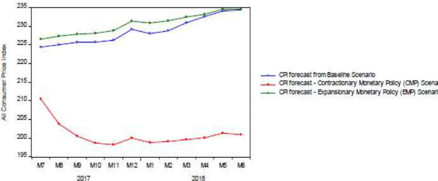
Effects of Monetary Policy Scenarios on All Items Consumer Price Index (CPI)

Figure 1 presents the forecast of all items CPI from July 2017 to June 2018 based on three

different scenarios (baseline, positive shock to M2 and negative shock to M2). With a positive

shock of 5% to monetary policy via broad money supply (M2), the CPI rises marginally above

the baseline scenario whereas a negative shock to M2 of the same magnitude leads to a huge

drop in all items CPI relative to the baseline scenario. Thus, upholding monetarist view on

inflation and supporting contractionary monetary policy as a veritable policy option for

achieving significant and consistent downward inflationary trend.

INSERT FIGURE 1 ABOUT HERE

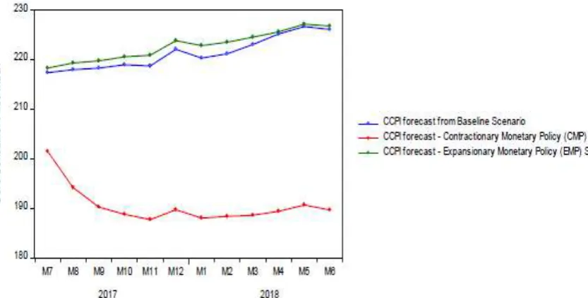
Effects of Monetary Policy Scenarios on Core Consumer Price Index (CCPI)

The response of the core CPI also follows the same pattern as the all item CPI. A positive shock

to M2 scenario leads to marginal increase in Core CPI above the baseline scenario but a similar

magnitude of negative shock yields a higher and consistent fall in the Core CPI (Figure 2).

INSERT FIGURE 2 ABOUT HERE

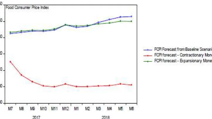
Effects of Monetary Policy Scenarios on Food Consumer Price Index (FCPI)

Figure 3 which presents the response of Food CPI to various types of shock to monetary

aggregates indicates that the response of Food CPI follows the same pattern as those of all item

CPI and Core CPI (Figure 3).

INSERT FIGURE 3 ABOUT HERE

4

5 Summary and Conclusion

Considering the adverse macroeconomic effect of inflation on welfare, fiscal budgeting, trade

performance, international competitiveness and the whole economy, it still remains a subject

of utmost concern and interest to policy makers. Thus, the historical path of inflation is not

only monitored by monetary authorities in both developed and developing countries, but

attempt is also often made to determine its future path. This is done by using various

methodologies which have been criticized to be defective in forecasting inflation. The large

number of macroeconomic variables included in forecasting inflation, according to the critics

of those methodologies, makes model selection cumbersome and difficult, hence the resort to

the use of BMA which obtained the best predictive performance averaging forecasts

constructed from several models. This study uses the Bayesian model averaging (BMA)

methodology to determine the predictors of inflation for Nigeria as well as forecast its future

path using a wide range of variables. The study derived eighteen (18) PCAs from sixty-three

(63) independent variables divided into ten groups and adopted the BMA and Frequentist

Model Averaging (FMA) as model averaging algorithms. Recognizing predictor variables as

either focused or auxiliary regressors, three different measures of inflation were estimated as

objective functions.

The results indicate that both in-sample and out-of-sample forecasts were highly

reliable judging from the various forecast performance criteria. The values of MSE were very

low (< 1.0) and ranges from 0.002 to 0.429; the mean forecast values of inflation rates were

very close to the actual values and the estimated credible intervals give 95% confidence that

inflation forecasts are within appreciable levels.

Various policy scenarios conducted were highly fascinating both from the theoretical

both positive and negative shocks to monetary aggregates moderate CPI inflation but with

higher magnitude for negative shocks. This study strongly recommends that, if the fiscal sector

is expected to maintain the current trend of expenditure up to June 2018, the Central Bank of

Nigeria, even with the objective of curtailing inflationary spiral, can embark on accommodative

monetary policy. This stems from the fact that it is capable, given the current economic

situation, of aiding recovery from recession without fueling inflation. It is however pertinent

to mention that restrictive monetary policy still proves more effective and efficient in curtailing

inflation.

References

Adams, S.O., Awujola, A. and Alumgudu, A.I. (2014). Modelling Nigeria’s Consumer Price Index using ARIMA Model. International Journal of Development and Economic

Sustainability, 2(2), 37 – 47.

Amadi, I. U., Gideon, W. O. & Nnoka, L. C. (2013). Time Series Models on Nigerian Monthly Inflation Rate Series. International Journal of Physical, Chemical and Mathematical Sciences, 2(2), 124-128.

Altug, S. and Cakmakli, C. (2015). Forecasting inflation using survey expectations and target inflation: Evidence for Brazil and Turkey. University of Amsterdam Working paper No IAAE2015-580.

Ang, A., Bekaert, G. and Wei, M. (2007). Do Macro Variables, Asset Markets, or Surveys Forecast Inflation Better? Journal of Monetary Economics, 54, 1163-1212.

Atkeson, A. and Ohanian, L.E. (2001). Are Phillips curves useful for forecasting inflation? Quarterly Federal Reserve Bank of Minneapolis, Winter 2001: pp. 1-12.

Bjornland, H.C., Gerdrup, K., Jore, A.S., Smith, C. and Thorsrud, L.A. (2009). Does forecast combination improve Norges Bank inflation forecasts? Working paper, Economics

Department, Norges Bank, Norway.

Blinder A.S. (1997). Is there a core of practical macroeconomics that we should all believe? American Economic Review, 87, 240-250.

Bruneau, C., DeBandt, O. and Flageollet, A. (2003). Forecasting inflation in the Euro area. Banque de France, Working paper series NER #102.

Buckland, S.T., Burnham, K.P. and Augustin, N.H. (1997). Model selection: an integral part of inference. Biometrics, 53, 603-618.

Chinonso, U.E. and Justice, O.I. (2016). Modelling Nigeria’s Urban and Rural Inflation

usingBox-Jenkins Model. Scientific Paper Series on Management, Economic Engineering in Agriculture and Rural Development, 16(4), pp 61 – 68.

Claeskens, G., and Hjort, N.L. (2003). The focused information criterion. Journal of the American Statistical Association, 98, 900-916.

Claeskens, G., and Hjort, N. L. (2008). Model selection and model averaging. Cambridge: Cambridge University Press.

Doguwa, I. S. and Alade, O. A. (2013). Short-term Inflation Forecasting Models in Nigeria. CBN Journal of Applied Statistics, 4(2), 1 – 29.

Duncan, R. and Martinez-Garcia, E. (2015). Forecasting Inflation with Global Inflation: When Economic Theory Meets the Facts. Paper presented at the 35th International Symposium on Forecasting, International Institute of Forecasters, Riverside, USA - June 21-24, 2015.

Fedderke, J. and Liu, Y. (2016). Inflation in South Africa: An assessment of alternative inflation models. South African Reserve Bank Working Paper series No. WP/16/03.

Figueiredo, F.M.D. (2010). Forecasting Brazilian inflation using a large dataset. The Banco Central do Brasil Working paper series No. 228.

Fujiwara, I. and Koga, M. (2002). A statistical forecasting method for inflation forecasting. Research and Statistics Department, Bank of Japan working paper 02-5.

Gaomab, M. (1998). Modelling inflation in Namibia. Bank of Namibia Occasional paper No. 1.

Giannone, D., Lenza, M., Momferatou, D. and Onorante, L. (2014). Short-term inflation projections: A Bayesian vector approach. International Journal of Forecasting, 30(3), 635- 644.

Groen J., Paap, R. and Ravazzolo, F. (2009). Real-time Inflation Forecasting in a Changing World. Econometric Institute Report, 2009-19, Erasmus University Rotterdam.

Hansen, B.E. (2007). Least Squares Model Averaging. Econometrica, 75, 1175-1189.

Hansen, B.E. (2008). Least-squares forecast averaging. Journal of Econometrics, 146(2), 342- 350.

Hansen, B.E. and Racine, J.S. (2012). Jackknife model averaging. Journal of Econometrics, 167(1), 38-46.

Hjort, N. L. and Claeskens, G. (2003). Frequentist model average estimators. Journal of the American Statistical Association, 98(464), 879-899.

Inam, U.S. (2017). Forecasting Inflation in Nigeria: A vector Autoregression Approach. International Journal of Economics, Commerce and Management, 5(1), 92 – 104.

Iwok, I.A. and Udoh, G.M. (2016). A Comparative study between the ARIMA-Fourier model and the Wavelet model. American Journal of Scientific and Industrial Research, 2016,

7(6):137-144.

John, E.E. and Patrick, U.U. (2016). Short-Term Forecasting of Nigeria Inflation Rates using Seasonal ARIMA Model. Science Journal of Applied Mathematics and Statistics, 4(3), 101- 107.

Kelikume, I. and Salami, A. (2014). Time Series Modeling and Forecasting Inflation: Evidence from Nigeria. The International Journal of Business and Finance Research, 8(2), 41 – 51.

Kuhe, D.A. and Egemba, R.C. (2016). Modelling and Forecasting CPI Inflation in Nigeria: Application of Autoregressive Integrated Moving average Homoskedastic Model. Journal of Scientific and engineering Research, 3(2), 57-66.

Lansing, K.J. (2002). Can the Phillips curve help forecast inflation?, FRBSF Economic Letter, Federal Reserve Bank of San Francisco, issue Oct 4.

Leamer, E.E. (1978). Specification Searches: Ad Hoc Inference with Nonexperimental Data, Wiley, New York.

Mallows, C.L. (1973). Some comments on C p. Technometrics, 15(4), 661-675.

Min, C.K. and Zellner, A. (1993). Bayesian and non-Bayesian methods for combining models and forecasts with applications to forecasting international growth rates. Journal of

Econometrics, 56(1-2), 89-118.

Moral‐ Benito, E. (2015). Model averaging in economics: An overview. Journal of Economic Surveys, 29(1), 46-75.

Okafor, C. and Shaibu, I. (2013). Application of ARIMA models to Nigerian Inflation dynamics. Research Journal of Finance and Accounting, 4(3): 138-150.

Omekara, C.O., Ekpenyong, E.J. and Ekerete, M.P. (2013). Modeling the Nigeria Inflation Rates using Periodogram and Fourier Series Analysis. CBN Journal of Applied Statistics, 4(2), 51-68.

Onimode, B.M., Alhassan, J.K. and Adepoju, S.A. (2015). Comparative Study of Inflation Rates Forecasting Using Feed-Forward Artificial Neural Networks and Auto-Regressive (AR) Models. International Journal of Computer Science Issues, 12(2), 260-266.

Otu, A.O., Osuji, G.A., Jude, O., Ifeyinwa, M.H. and Andrew, I.I. (2014). Application of

SARIMA Models in Modeling and Forecasting Nigeria’s Inflation Rates. American Journal of Applied mathematics and Statistics, 2(1), 16 – 28.

Stock, J.H. and Watson, M.W. (1999). Forecasting inflation. Journal of Monetary Economics, 44(2), 293-335.

Stock, J. H. and Watson, M.W. (2004). Combination forecasts of output growth in a seven‐ country data set. Journal of Forecasting, 23(6), 405-430.

Stock, J.H. and Watson, M.W. (2005). An empirical comparison of methods for forecasting using many predictors. Manuscript, Princeton University.

Stock, J.H. and Watson, M.W. (2006). Forecasting with many predictors. Handbook of economic forecasting, 1, 515-554.

Stock J. H. and Watson, M.W. (2008). Philips Curve Inflation Forecasts. NBER Working Paper No. 14322. vs. 0.3.0, URL: http://cran.r-project.org/web/packages/BMS/

Sims, C.A. (2002). The role of models and probabilities in the monetary policy process. Brookings Papers on Economic Activity, 1-40.

Waiquamdee, A. (2001). Modelling the inflation process in Thailand. BIS Papers No. 8: 252- 263.

Wright, J.H. (2008). Bayesian model averaging and exchange rate forecasts. Journal of Econometrics, 146(2), 329-341.

Wright, J. H. (2009). Forecasting US inflation by Bayesian model averaging. Journal of Forecasting, 28(2), 131-144.

Yemitan, R.A. and Shittu, O.I. (2015). Forecasting Inflation in Nigeria by State Space Modeling. International Journal of Scientific and Engineering Research, 6(8), 778-786.

Younus, S. and Roy, A. (2016). Forecasting inflation and output in Bangladesh: Evidence from a VAR model. Research department and Monetary Policy Department of Bangladesh Bank Working Paper series WP No. 1610.

Table 1: Variable groupings

Monetary aggregates Real Sector indicators Interest rates

Seven-day (7D) Credit to private sector (CPS) Real GDP (RGDP) One month (1M) Net credit to FGN (NCG) Nominal GDP (NGDP) Three-month (3M) Foreign assets to DMBs (FA) Real Private Capital Expenditure (RPCE) Six-month (6M) Broad money supply (M2) Nominal Private Capital Expenditure

(NPCE)

Twelve-month (12M) Narrow money supply (M1) Average deposit rate (DR) Broad money growth rate (M2g) Seasonally Adj. Series Average lending rate (ALR) Growth rate of M2 (M2g) Real GDP (RGDP_D) Prime lending rate (PLR) Reserve money (RM) Nominal GDP (NGDP_D) Maximum lending rate (MLR)

Real PCE (RPCE_D) Monetary policy rate (MPR) Seasonally Adj. Series Nominal PCE (NPCE_D) Treasury bills rate (TB) Credit to private sector (CPS_D)

Broad money supply (M2_D) Narrow money supply (M1_D) Reserve money (RM_D) Foreign assets to DMBs (FA_D)

Exchange rate indices Capital market indicators Prices

Official exchange rate (EXR) All share index (ASI) Core CPI (CCPI) BDC exchange rate (EXRB) Market capitalization (MC) Food CPI (FCPI) Nominal effect. exch. rate

(NEER)

Bond yields (BR) All items CPI (CPI) Real effective exchange rate

(REER)

Inflation rate (INF) Inflation expectations (IFE) Price of PMS (PMS/ltr)

External sector indicators Agricultural indicators Fiscal indicators

Foreign reserve (FER) Average rainfall (ARF) Federal account allocation (FAAC)

Imports (IM) Nominal Agric. Production (ANY) Fiscal deficit to GDP ratio (FPGDP)

Import growth rates (IMg) Real Agric. Production (RAY) FGN Total Expenditure (GE) Exports (EX)

Export growth rates (EXg) Seasonally Adj. Series Seasonally Adj. Series Terms of trade (TOT) Nominal Agric. Production (ANY_D) Federal account allocation

(FAAC_D)

Real Agric. Production (ARY_D) FGN Total Expenditure (GE_D) Seasonally Adjusted Series

Imports (IM_D) Exports (EX_D)

International indicators

Table 2: Characteristics of the extracted Principal components

Seasonally Unadj. Series Seasonally adj. series Indicator Components Rotated

eigenvalue

% Total variance

Cum. %

Components Rotated eigenvalue

% Total variance

Cum. %

Monetary aggregates

1 6.302 70.02 70.02 1 4.758 95.168 95.168

2 1.437 15.96 85.98

3 1.028 11.42 97.40

Interest rates 1 7.698 64.149 64.149

2 2.138 17.814 81.963

Real sector 1 3.571 89.270 89.270 1 3.624 90.600 90.600

Exchange rates

1 1.962 98.085 98.085

Capital market

1 1.693 84.643 84.643

Prices 1 4.417 63.100 63.100

2 1.985 28.356 91.457

Agricultural sector

1 2.094 69.797 69.797 1 1.993 99.630 99.630

Fiscal 1 1.891 63.045 63.045 1 1.589 79.458 79.458

External sector

1 2.577 42.945 42.945 1 1.786 89.321 89.321

2 1.289 21.485 64.430

Table 3: Identified principal components showing variables

Seasonally Unadj. series (Component correlations)

Seasonally adj. series (Component correlations)

Indicator Variables 1 2 3 Variables 1 2 3

Monetary aggregates CPS .985 - - CPS_D 0.997 - - M2 .979 - - M2_D 0.995 - - DD .975 - - M1_D 0.982 - - M1s .955 - - FA_D 0.957 - - RM .950 - - RM_D 0.946 - - FA .915 - -

M1g - .832 - M2g - .760 - NCG - - .910 Interest rates M6 0.948 - -

M3 0.944 - - 7D 0.944 - - M12 0.918 - - M1 0.917 - - M12 0.842 - - PLR 0.842 - - MPR 0.740 - - DR 0.677 - - TB 0.633 - - MLR - 0.855 - ALR - 0.710 -

Real sector NGDP 0.981 - - NGDP_D 0.984 - - NPCE 0.980 - - NPCE_D 0.983 - - RGDP 0.964 - - RGDP_D 0.968 - - RPCE 0.848 - - RPCE_D 0.867 - - Exchange rates EXR 0.990 - -

EXRB 0.990 - - Capital market indicator ASI 0.920 - - MC 0.920 - - Prices CCPI 0.990 - - CPI 0.989 - - FCPI 0.985 - - PMS 0.958 - - WFPI 0.753 - - IFE - 0.970 - INF - 0.970 -

Agricultural indicator ARF 0.983 - - ANY_D 0.998 - - ANY 0.937 - - ARY_D 0.998 - - ARY 0.501 - -

Fiscal indicator GEX 0.937 - - GEX_D 0.891 FPGDP -0.736 - - FAAC_D 0.891 FAAC 0.687 - -

External sector indicator IM 0.894 - - IM_D 0.945 - - EX 0.788 - - EX_D 0.945 - - FER 0.687 - -

Table 4: Forecasts for CPI

Period Actual

Mean forecast

Std forecast

MSE

forecast 5% CI 95% CI

2016M03 189.94 186.91 3.368 0.078 180.96 192.87

2016M04 192.99 189.23 3.361 0.064 183.38 195.09

2016M05 198.3 201.11 3.613 0.075 194.07 208.15

2016M06 201.7 206.58 3.861 0.043 196.63 215.81

2016M07 204.23 213.64 4.356 0.024 200.15 227.44

2016M08 206.29 217.78 4.668 0.019 203.25 236.05

2016M09 207.96 221.31 4.884 0.016 206.23 Infinity 2016M10 209.68 224.52 5.182 0.014 208.82 Infinity 2016M11 211.33 221.91 4.829 0.021 206.78 Infinity

2016M12 213.56 226.93 5.060 0.016 211.26 246.69

2017M01 215.72 228.97 5.433 0.016 212.18 Infinity

2017M02 218.95 230.43 5.384 0.018 213.84 250.17

2017M03 222.71 227.66 4.842 0.032 213.58 240.76

2017M04 226.27 224.48 4.690 0.055 211.96 236.01

2017M05 230.53 228.35 4.629 0.057 216.37 239.44

2017M06 234.17 230.48 4.507 0.058 219.75 240.52

Table 5: Forecasts for CCPI

Period Actual

Mean forecast

Std forecast

MSE

forecast 5% CI 95% CI

2016M03 186.42 185.21 3.766 0.097 178.71 191.70

2016M04 189.55 186.78 3.734 0.080 180.51 193.08

2016M05 194.7 203.36 3.995 0.012 196.40 210.35

2016M06 198.27 209.56 4.132 0.293 202.52 216.64

2016M07 200.69 218.83 4.516 0.0135 210.56 227.06

2016M08 202.4 222.89 4.876 0.0147 213.18 232.59

2016M09 204.34 227.00 5.068 0.0079 216.64 237.43

2016M10 205.86 231.12 5.383 0.0079 219.13 243.40

2016M11 207.33 227.60 5.008 0.042 216.72 238.67

2016M12 208.61 232.48 5.335 0.011 221.00 244.10

2017M01 210.03 235.25 5.734 0.007 223.93 246.55

2017M02 212.34 236.22 5.795 0.014 224.92 247.45

2017M03 215.14 231.53 5.259 0.147 221.82 241.21

2017M04 217.51 229.29 5.074 0.828 219.91 238.60

2017M05 220.05 232.73 4.988 0.508 223.70 241.73

Table 6: Forecasts for FCPI

Period Actual

Mean forecast

Std forecast

MSE

forecast 5% CI 95% CI

2016M03 194.87 189.48 3.759 0.0406 182.77 196.27

2016M04 197.40 192.32 3.751 0.0443 185.73 198.97

2016M05 202.46 200.22 4.006 0.0732 192.49 208.24

2016M06 205.39 203.53 4.233 0.0540 193.90 214.68

2016M07 207.87 207.59 4.795 0.0356 195.00 224.65

2016M08 210.30 210.84 5.113 0.0290 196.91 230.48

2016M09 212.00 213.47 5.338 0.0255 198.73 234.56

2016M10 213.82 215.00 5.685 0.0225 198.97 Infinity

2016M11 215.70 214.17 5.290 0.0292 199.57 235.04

2016M12 218.58 219.45 5.421 0.0263 204.64 239.86

2017M01 221.40 218.04 5.925 0.0258 201.26 Infinity

2017M02 225.81 220.58 5.819 0.0276 204.56 242.30

2017M03 230.80 221.29 5.235 0.0249 207.87 237.76

2017M04 235.50 218.90 5.089 0.0073 206.36 233.51

2017M05 241.47 223.05 5.065 0.0047 210.67 237.29