A Perfect Specialization Model for Gravity Equation in Bilateral Trade based on Production Structure

Munich Personal RePEc Archive

A Perfect Specialization Model for

Gravity Equation in Bilateral Trade

based on Production Structure

Einian, Majid and Ravasan, Farshad

Graduate School of Management and Economics, Sharif University

of Technology„ Paris School of Economics

30 June 2016

A Perfect Specialization Model for Gravity Equation in Bilateral

Trade based on Production Structure

Majid Einian

Graduate School of Management and Economics, Sharif University of Technology, Tehran, Iran.

Corresponding author, email: [email protected]

Farshad Ranjbar Ravasan

Paris School of Economics, Paris, France

1 _{This work of research has not been funded by any organization or institution. We hereby}

1

A Perfect Specialization Model for Gravity Equation in Bilateral

Trade based on Production Structure

Abstract

Specialization models are important in providing a solid theoretical ground for

gravity equation in bilateral trade. Some research papers try to improve

specialization models by adding imperfect specialization to them, but we believe

it is unnecessary complication. We provide a perfect specialization model based

on the phenomenon that we call tradability, which overcomes the problems with

simpler models. We provide empirical evidence using estimations on panel data

of bilateral trade of 40 countries over 10 years that support the theoretical model.

Keywords: bilateral trade, gravity equation, perfect specialization, tradability.

JEL classification: F11, F14, C23, E23.

Introduction

Studying trade is one of the most important branches of economics. Although it is as old

as economics itself (since Ricardo [1819]), it is gaining much more importance as

international trade has been growing tremendously. Gravity equation is a form of

empirical relation explaining the flow of bilateral trade by the size of two engaging

countries and negatively by distance between them usually in a form resembling the law

of gravity in Physics. The traditional relationship did not have a theoretical basis, but

theories of trade have tried to explain this equation (Deardorff 1998).

There are a lot of theories, which try to explain the pattern of international trade.

A branch of these theories are based on relative factor abundance. One of the common

relative-factor-abundance models is the Heckscher-Ohlin model. This theory predicts

that trade patterns would be based on relative factor advantages. Those countries with a

2

comparatively large amount of that factor in their GDP. Although this model generally

is accepted as the theory of trade but does not satisfy empirical results (Bergstrand

1989).

A study by Wassily Leontief indicates that the exports of United States as the

most capital endowed country included more labour intensive commodities, which

suggests the opposite result. This contradiction is known as the Leontief paradox. The

Leontief paradox makes doubt about that Heckscher-Ohlin works in the real world.

An alternative theory, first proposed by Linder (1961), claims that the pattern of

trade is determined by similarity of two country’s preferences (Bohman and Nilson

2007). Countries with similar demand develop similar industries that result in producing

similar goods and services. These countries continue trade in differentiated but similar

goods. Linder (1961) writes, “The more similar the demand structure of the two

countries the more intensive potentially is the trade between these two countries.”

Importance of Linder's hypothesis considering demand part is what departs it from

neoclassical theories of trade, which pay attention only to production features' part.

Linder suggests that per capita income can be used as a proxy for preferences. The

hypothesis can then be tested by comparing per capita income between trading partners.

It means the more similar two country’s GDP’s are, the more they trade. That result is

consistent with the gravity equation.

Helpman and Krugman (1985) develop the Lender’s idea. They observed that

countries with similar levels of income trade more (Bohman and Nilson 2006). This is

not supported by Heckscher-Ohlin model of trade and comparative advantage theory.

They introduced Increasing Returns to Scale as the fundamental factor that account for

part of trade known as intra-industry trade. They relax the neoclassical assumption,

3

different approaches. First is the Marshallian approach, where the economies of scale is

assumed external to firms; second is the Chamberlinian approach, where imperfect

competition takes the relatively tractable form of monopolistic competition; and the

third one is the Cournot approach of non-cooperative quantity-setting firms.

The reciprocal dumping model – in which both countries export the same good

to each other to gain higher profits by supplying their product to the other country with

lower prices than their own market (Krugman and Obstfeld 2009) – also explains

gravity equation. Feenstra, Markusen, and Rose (1998) provided evidence for reciprocal

dumping by assessing the “home market effect” in separate gravity equations for

differentiated and homogeneous goods. The home market effect showed a relationship

in the gravity estimation for differentiated goods, but showed the inverse relationship

for homogeneous goods. The authors show that this result matches the theoretical

predictions of reciprocal dumping playing a role in homogeneous markets.

At all, the literature about the gravity model of trade includes two debates: first

what model is the theoretical base of gravity equation and second what factors account

for deviation of actual bilateral trade from gravity form. To answer the first question,

Deardorff (1998) claims that the basic gravity model can be derived from

Heckscher-Ohlin as well as the Linder and Helpman-Krugman hypotheses. Deardorff (1998)

concludes that, considering how many models can be tied to the gravity model equation;

it is not useful for evaluating the empirical validity of theories. Barriers, Demand

structure, and imperfect specialization are three factors, which were noticed as basic

factors for deviation from gravity equation.

To answer the second question Evenett and Keller (2002) suggest that relaxing

the perfect specialization assumption produces much better results. They support an

4

conditions, first the model should provide a regression coefficient less than one, i.e. can

match the real-world data; and second the model should be consistent with the

correlation of specialization index and the regression coefficient. As we mentioned the

first condition is a kind of gravity-equation-support-identification and the second one

checks if the model can provide an explanation for actual bilateral trade deviations from

traditional gravity equation. We provide a perfect specialization model based on the

phenomenon that we call tradability, which explains the less-than-one coefficient by

non-tradeable share of GDP rather than levels of specialization. We provide empirical

evidence using estimations on panel data of bilateral trade of 40 countries over 10 years

that support the theoretical model. We also provide some empirical evidence on how

imperfect specialization might not address the fundamental deviation factor since high

correlation of specialization index with other important deviation factors like trade cost

and barriers. The remainder of the paper is structured as follows. In the section 2, we

review Evenett and Keller's model identification approach. Then we introduce our

model of perfect specialization based on the tradability phenomenon in section 3.

Section 4 provides information about data used for the study and also the tradability

index we calculated for 40 countries. Section 5 gives the empirical test results. And

section 6 concludes.

Model Identification Approach

Evenett and Keller's identification approach consists of two steps based on a regression

of this type:

𝑋𝑎𝑏 = 𝛼(𝑋𝑎𝑏𝑀𝑜𝑑𝑒𝑙) + 𝜀𝑎𝑏 (1)

5

If we ignore the theoretic base of each specialization model, Evenett and Keller

suggest that all perfect specialization models will lead in a gravity equation as in

follows:

𝑋𝑎𝑏 = 𝑌𝑎_𝑌×𝑌_𝑤𝑏 (2)

in which 𝑋 is export volume, 𝑌 is the gross domestic product and 𝑎, 𝑏, and 𝑤 indices

are respectively indicators of exporting country, importing country, and the world. As

obvious in eq. 2, the coefficient of the fraction is equal to one, i.e. if this is the true

model, estimated 𝛼 in regression in eq. 1 will be not be significantly different from one.

Evenett and Keller (2002) give gravity equations in form of eq. 3 and eq. 4 based on

two different imperfect specialization models.

𝑋𝑎𝑏 = (1 − 𝛾𝑎)𝑌𝑎_𝑌×𝑌_𝑤𝑏 (3)

𝑋𝑎𝑏 = (𝛾𝑏− 𝛾𝑎)𝑌𝑎_𝑌×𝑌_𝑤𝑏 (4)

in which 𝛾 is the specialization index (a number between 0 and 1). As obvious, the

coefficient of the fraction in these models is less than one. Evenett and Keller has

shown that this coefficient is indeed less than one in bilateral trade data. They conclude

thus that perfect specialization models are incapable of explaining the data regarding

this coefficient.

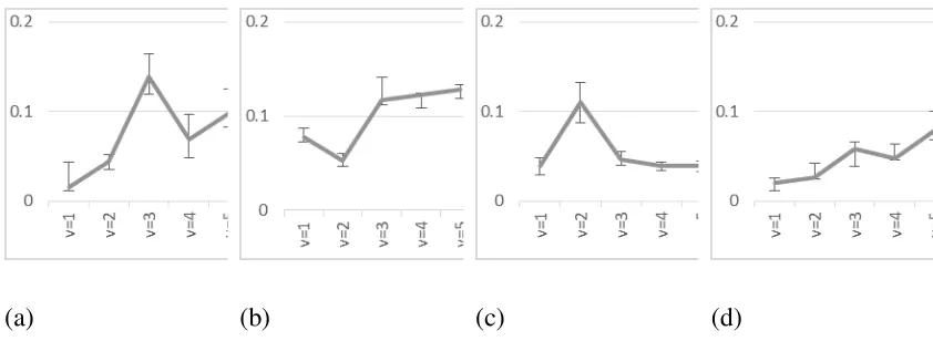
The second criteria in Evenett and Keller (2002) is that the model should

provide reasons why the coefficient departs from 1. They run different regressions to

estimate the coefficient of the fraction from data using five different levels of

6

estimates of coefficient of the fraction. Their results are summarized in panels (a) to (d)

of Figure 1, and shows a weak relationship.

A Model of Gravity with Perfect Specialization based on

Tradable/Non-tradable Product Distinction

Assume that there are three goods in world named as s, t and z. Assume that s is not

tradeable and so to be precise we should use different notation for product s of each

country. Assuming that there are two countries a and b, we call the s produced and

consumed in country a: 𝑠_𝑎, and the s produced and consumed in country b: 𝑠_𝑏. Either

reason of perfect specialization, namely IRS forces or H-O model forces, can be

assumed as the reason for perfect specialization in tradable goods in model. Perfect

specialization leads to each country to produce either of t or z. We assume that a is

producing t and b is producing z.

So these countries GDP’s are:

𝑌𝑎 = 𝑡 + 𝑠𝑎 (5)

𝑌𝑏 = 𝑧 + 𝑠𝑏 (6)

and so letting 𝜆's denote tradable share of GDP we have:

𝜆𝑎 =_𝑌𝑡_𝑎 =_𝑡+𝑠𝑡_𝑎 (7)

𝜆𝑏= _𝑌𝑧_𝑏= _𝑧+𝑠𝑧_𝑏 (8)

Supposing identical homothetic preferences, we have that each country's share in

consumption of each commodity is equal to its share of world GDP, i.e.

7

To simplify the perfect specialization model, Evenett and Keller (2002) assume that the

share of non-tradable goods in GDP is identical for all countries. We do not simplify

further as we believe that the idea of tradeable share of GDP plays a great role in

forming gravity equation and any simplification might lead to unreasonable results.

Thus our model leads in a gravity equation with a coefficient of the ratio less than 1. To

support the second criteria we shall show that the deviation of estimate of coefficient of

the ratio is related to the share of non-tradable production in GDP. To show this we take

logarithms of eq. 9 to get:

ln(𝑋𝑎𝑏) = 𝛽0+ 𝛽1ln 𝜆𝑎 + 𝛽2ln(𝑌𝑎_𝑌×𝑌_𝑤𝑏) + 𝜀 (10)

Which is in fact the logarithm of eq. 11:

𝑋𝑎𝑏 = 𝑒𝛽0 × 𝜆𝑎𝛽1× (𝑌𝑎_𝑌×𝑌_𝑤𝑏) 𝛽2

(11)

Thus 𝛽̂₁ = 𝛽̂₂ = 1 shows complete accordance of the model to the data. On the other

hand tradable production share in GDP is important only if 𝛽̂₁ is statistically significant.

Data

World commodity trade data are gathered from UN ComTrade and UN Service Trade

data set provides the data on trade of services. National account data are from World

Development Indicators data set. 40 countries are selected that constitute a large part of

world GDP (about 90%) and world trade. Saudi Arabia and Israel are dropped because

of technical problems such as missing data. Table 2 lists the countries used for this

study. The data form a panel of 1600 (40x40) export relationship over 10 years

8

Calculating Tradable Productions Share

Model proposed in this paper is based on the tradeable production share in GDP,

so we shall provide some data on this phenomenon. However, in reality, no data are

gathered for tradability. We only observe traded goods and services, not what was

potentially tradable. We study sectors of production and compare the shares of each

sector in world production and world trade and decide if that section is tradable. For

example, agriculture constitutes about 5.61 percent of the world trade, but only 3.35

percent of world GDP, thus we can say that agriculture is tradeable. Adding up tradable

sectors, we can calculate the tradability index of each country. Even so, these

calculations are not precise because of absolute decision on tradability of sectors.

Textiles' share, as an example, is less than 0.5 percent of world GDP, yet more than 6

percent in world trade, so in fact textile is much more tradable than agriculture. So we

use relative tradability with comparing the shares with the most tradable sector

(textiles). So if 100 percent of textile is considered tradable, 81% of chemical and

12.36% of agricultural products are tradable. On the other hand, only 2.31 percent of

services (which is considered a non-tradable sector) are tradable.

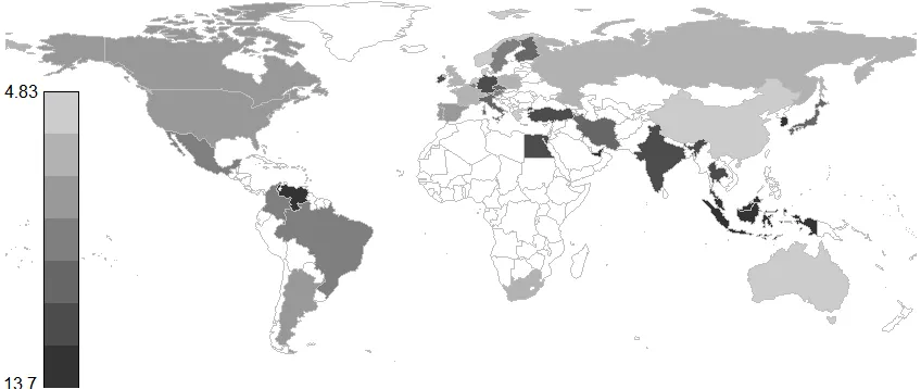
We use the data from Table 1 to calculate the tradability index for each country

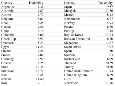
in each year. Table 2 reports the average tradability index for countries of the study

from 2000 to 2009. As shown in this table, Indonesia, Singapore, Malaysia, and South

Korea had the highest indices. This means that these countries have production

structures that are able to export more. The calculated index is not based on trade data

of these countries and is only based on the production structure. Data in Table 2, is

plotted on the map of the world in Figure 2.

The Results

9

panel is unbalanced by nature (not all countries have exported to all countries in every

year). 6624 observations are available. We estimated the equation using both fixed

effect model and random effect model. Testing the null hypothesis that no panel effects

exits (thus recommending use of pooled estimates) is rejected. Hausman (1978) test

indicates that panel effects are fixed effects, and random effects estimations leads to

biased estimates of the equation (Baltagi 2008). Table 3 reports the results of the both

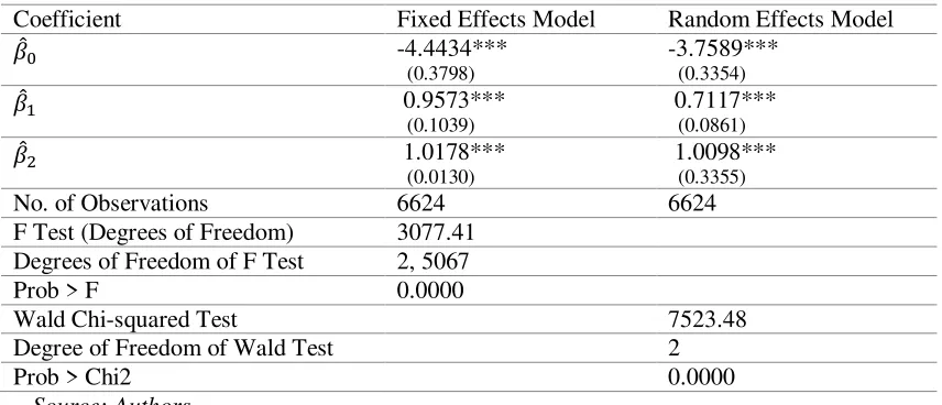
models and Hausman test results are reported in Table 4. As we can see in Table 3, both

coefficients of interest 𝛽̂₁ and 𝛽̂₂ are statistically not different than 1, thus the theoretic

model is supported with data. 𝛽̂₂ = 1 means that the core part of the gravity equation,

i.e. that trade is positively related to the multiplication of GDP of both partners is

modelled in a way that is completely compatible with data. 𝛽̂₁ = 1 means that the

tradability index is the sole reason for deviations of data from basic perfect

specialization models.

Conclusion

We provided a perfect specialization model based on the tradability phenomenon, which

does not have the problems indicated by Evenett and Keller (2002), namely that our

perfect specialization model totally explains the deviations of data from simpler perfect

specialization models without entrapment in the complexities of imperfect

specialization models (which we do not believe are doing any good in explaining the

data). Empirical evidence using estimations on panel data of bilateral trade of 40

countries over 10 years totally and fully supports the theoretical model. In the process of

providing empirical evidence, we built and reported an index of tradability, which is a

10

References

Bergstrand, J.H (1989). "The Generalized Gravity Equation, Monopolistic Competition

and the Factor-Proportions Theory in International Trade." The Review of Economics

and Statistics. 71(1): 143-153.

Bohman H, & Nilson, D. (2007) "Market Overlap and the Direction of Exports: A New

Approach of Assessing the Linder Hypothesis." Working Paper Series in Economics

and Institutions of Innovation. 86. Royal Institute of Technology.

Deardorff, A. (1998). "Determinants of Bilateral Trade: Does Gravity Work in a

Neoclassical World?", in The Regionalization of the World Economy, edited by J.A.

Frankel. Chicago: Univ. Chicago Press for National Bureau of Economic Research.

7-32.

Evenett, S. J., & Keller, W. (2002). "On Theories Explaining the Success of the Gravity

Equation." Journal of Political Economy, 110 (2): 281-361.

Feenstra, R. C., Markusen, J. A., & Rose, A. K. (1998). Understanding the home market

effect and the gravity equation: The role of differentiating goods (No. w6804). National

Bureau of Economic Research.

Hausman, J. A. (1978). "Specification tests in econometrics," Econometrica, 46(6):

1251-1271.

Helpman, E., & Krugman, P. R. (1985). Market structure and foreign trade: Increasing

returns, imperfect competition, and the international economy. MIT press.

Krugman, P. R., & Obstfeld, M. (2009). International Economics: Theory and Policy.

11

Linder S.B. (1961). An Essay on Trade and Transformations. Stockholm: Almqvist &

Wiksell.

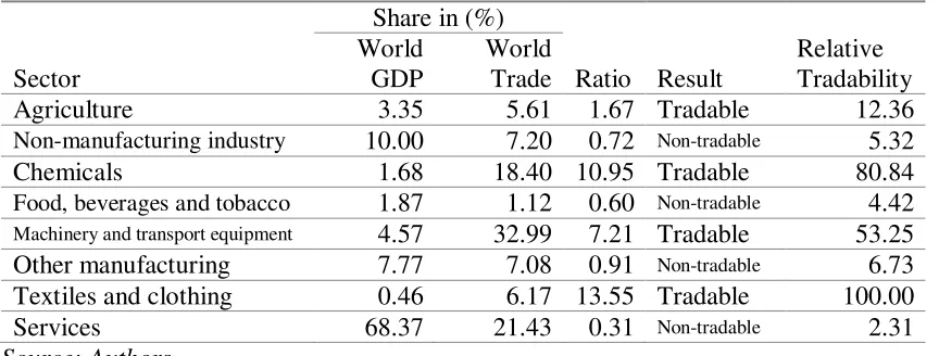
12 Table 1: Tradability of Each Economic Sector

Sector

Share in (%)

Ratio Result

Relative Tradability World

GDP

World Trade

Agriculture 3.35 5.61 1.67 Tradable 12.36

Non-manufacturing industry 10.00 7.20 0.72 Non-tradable _5.32

Chemicals 1.68 18.40 10.95 Tradable 80.84

Food, beverages and tobacco 1.87 1.12 0.60 Non-tradable _4.42 Machinery and transport equipment 4.57 32.99 7.21 Tradable 53.25 Other manufacturing 7.77 7.08 0.91 Non-tradable _6.73 Textiles and clothing 0.46 6.17 13.55 Tradable 100.00

Services 68.37 21.43 0.31 Non-tradable _2.31

13

Table 2: Average of 2000-2009 Tradability Index for 40 Countries

Country Tradability Country Tradability

Argentina 7.31 Japan 9.57

Australia 4.83 Malaysia 13.56

Austria 7.77 Mexico 8.12

Belgium 8.03 Netherlands 6.27

Brazil 8.25 Norway 5.93

Canada 7.56 Poland 6.86

China 6.19 Portugal 7.45

Colombia 8.00 Rep. of Korea 13.24 Czech Rep. 8.92 Russian Federation 6.70

Denmark 5.27 Singapore 13.67

Egypt 11.24 South Africa 7.02

Finland 9.21 Spain 7.50

France 7.04 Sweden 7.63

Germany 9.99 Switzerland 6.99

Greece 5.25 Thailand 10.59

India 10.35 Turkey 10.60

Indonesia 13.74 United Arab Emirates 11.94 Iran 8.45 United Kingdom 6.69

Ireland 11.40 USA 7.10

Italy 9.13 Venezuela 11.76

14

Table 3: Estimating the Gravity Equation based on Imperfect Specialization Model of

Bilateral Trade; Fixed and Random Effect Models

Coefficient Fixed Effects Model Random Effects Model

𝛽̂0 -4.4434***

(0.3798)

-3.7589***

(0.3354)

𝛽̂1 0.9573***

(0.1039)

0.7117***

(0.0861)

𝛽̂2 1.0178***

(0.0130)

1.0098***

(0.3355)

No. of Observations 6624 6624 F Test (Degrees of Freedom) 3077.41

Degrees of Freedom of F Test 2, 5067 Prob > F 0.0000

Wald Chi-squared Test 7523.48

Degree of Freedom of Wald Test 2

Prob > Chi2 0.0000

15

(a) (b) (c) (d)

Figure 1. Estimates of Coefficients of Gravity Equation versus Specialization Level.

16

Figure (2) Average of 2000-2009 Tradability Index for 40 Countries