Article
1
Iterative positioning algorithm of the target node
2
based on distance correction in WSN
3
Jing Chen
1,2,*, Shixin Wang
1, Mingsan Ouyang
1,* Yudi Chen
2and Yuting Xuan
14
1 School of Electrical and Information Engineering, Anhui University of Science and Technology, No.168,
5
Taifeng Road, Huainan 232001, China; [email protected] (S.W.); [email protected] (Y.X.)
6
2 Department of Electrical Engineering and Electronics, University of Liverpool, Liverpool L69 3BX, United
7
Kingdom
8
3 Department of Electrical and Electronics Engineering, Xi’an Jiaotong- Liverpool University, Suzhou 215123,
9
China; [email protected] (Y.C.)
10
* Correspondence: [email protected] (J.C.); [email protected] (M.O.)
11
Received: date; Accepted: date; Published: date
12
Abstract: The node position information is critical in the wireless sensor network (WSN). However,
13
the existing positioning algorithms commonly have low positioning accuracy because of noise
14
interferences in communication. To solve this problem, this paper presents an iterative positioning
15
model based on distance correction to improve the positioning accuracy of the target node in WSN.
16
First, the log-distance distribution model of received signal strength indication (RSSI) ranging is
17
built and the noise impact factor is derived based on the model. Second, the initial position
18
coordinates of the target node are obtained based on the triangle centroid localization algorithm,
19
thereby calculating the distance deviation coefficient under the influence of noise. Then, the ratio of
20
the distance measured by the log-normal distribution model to the median distance deviation
21
coefficient is taken as the new distance between the anchor node and the target node. Based on the
22
new distance, the triangular centroid positioning algorithm is used again to calculate the target
23
node coordinates. Finally, the iterative positioning model is constructed, and the distance deviation
24
coefficient is updated repeatedly to update the positioning result until the set number of iterations
25
is reached. Experiment results show that the proposed iterative positioning model can improve
26
positioning accuracy effectively.
27
Keywords: iterative positioning algorithm; distance correction; RSSI; noise impact factor; distance
28
deviation coefficient
29 30
1. Introduction
31
Wireless sensor network has been applied widely in various fields of defense, industry and
32
social life due to its advantages of low power consumption, low cost, self-organization and so on. In
33
order to provide effective monitoring services in engineering applications, the nodes own position
34
information must be provided [1,1]. The node position information is the key to whether the
35
information obtained is valuable or not in WSN, especially for the target reconnaissance and
36
tracking in the field of military and anti-terrorism [3,4]. It can be said that perceived data are
37
meaningless if no node position information are provided. However, in the actual physical
38
environment, the wireless signals are inevitably interfered by noises such as multi-path fading [5,6],
39
diffraction [7], antenna gain [8], non-line of sight [9] and so on in the process of propagating, and
40
uncertain propagation loss is produced, which results in inaccuracy in ranging. The maximum
41
ranging error is up to ±50% [10].
42
To solve this problem, the node positioning method in WSN should be explored deeply. An
43
effective node positioning method must consider the following problems. (1) How to construct a
44
mathematical model to fit the nonlinear relationship between the RSSI and the distance? (2) What
45
© 2019 by the author(s). Distributed under a Creative Commons CC BY license.
kind of positioning algorithm should be used to obtain more accurate positioning accuracy? (3)
46
What are the basic requirements to consider in terms of hardware resources and computational
47
complexity when building a positioning algorithm?
48
Based on the above three problems, we proposed the target node iterative positioning
49
algorithm based on distance correction in this paper. The motivation of this paper is reducing the
50
positioning error of the target node to help users obtain accurate position information. The process
51
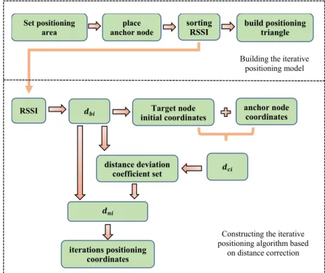
of the target node iterative positioning model based on distance correction is shown as Figure 1.
52
53
Figure 1. The process of the target node iterative positioning model based on distance correction
54
In our proposed algorithm, the median of the distance deviation coefficients is used to modify
55
the measured distance during each iteration. The median of the distance deviation coefficients can
56
more closely express the overall distance deviation characteristic. The log-distance distribution
57
model is used to calculate the distance between unknown target nodes and connected anchor nodes
58
in order to fit the nonlinear relationship between distance and RSSI more accurately, and reduce
59
computational complexity. The iterative positioning model is constructed to ensure that the target
60
node is in the area enclosed by the connected anchor nodes, which is also of great help to improve
61
the positioning accuracy. In addition, the node iterative positioning algorithm based on distance
62
correction can provide theoretical support for future research. Contributions are included in the
63
following aspects.
64
(1) Derivation of noise impact factor based on log-normal distribution model
65
The expression of the noise impact factor FN is derived by reconstructing mathematical model,
66
which is the corresponding numerical relationship between the noise impact factor FN and the
67
measured distance. The noise impact factor proposed in this paper is used to describe the
68
influence degree of noise on the measured values of RSSI.
69
(2) The selection of distance deviation coefficient on node measured distance
70
The distance deviation coefficient is used to evaluate the deviation degree of the distances
71
calculated by the log-distance distribution model and the triangle centroid algorithm
72
respectively, and a distance deviation coefficients set is established. The median of the distance
73
deviation coefficient set is selected to characterize the deviation degree of the whole node
74
measured distances, which can better reflect the overall distance deviation characteristic.
75
RSSI Target node
initial coordinates
anchor node coordinates
distance deviation coefficient set
iterations positioning coordinates Set positioning
area
sorting RSSI
build positioning triangle place
anchor node
Building the iterative positioning model
Constructing the iterative positioning algorithm based
on distance correction
(3) Construction of the iterative positioning algorithm based on distance correction
76
The distance deviation coefficient median is used as an iteration factor for the iterative
77
positioning algorithm. In the process of each iteration, the median of the distance deviation
78
coefficients is used to correct the distance from the last positioning, obtaining a distance value
79
closer to the true value. The triangle centroid localization algorithm is iteratively used to reduce
80
the positioning fluctuation error and improve positioning accuracy.
81
The rest of the paper has been organized as follows: Section 2 will demonstrate a brief review of
82
related works. The proposed iterative positioning algorithm will be provided in Section 3. The
83
iterative positioning model will be constructed in Section 4. The experimental results and some
84
analysis will be given in Section 5. Finally, key conclusions and the general discussion will be
85
summarized in Section 6.
86
2. Related works
87
This section reviews two existing works which are the reference foundation theory for
88
positioning of the target node in WSN. First is the measurement of the distance between the target
89
node and the anchor node. Second is to determine the position coordinates of the target node.
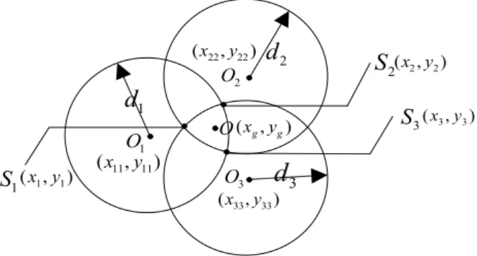
90
2.1. The measurement of distance between the target node and the anchor node
91
The measurement of distance between the target node and the anchor node is an important
92
research topic of the node positioning in WSN. Nowadays, most of the existing node positioning
93
algorithms can be divided into two categories according to whether it is necessary to measure the
94
distance or angle. One is the range-based measurement positioning algorithm and the other is
95
range-free measurement positioning algorithm [11]. The distance measurement refers to calculating
96
the distance or orientation between the unknown target node and the anchor node connected thereto
97
through communication between them [12]. The classical distance measurement algorithms include
98
based on signal time of arrival (TOA), signal time difference of arrival (TDOA) [13], Angle of Arrival
99
(AOA) [14] and received signal strength (RSSI) [15,16] algorithms.
100
The first three algorithms need to accurately calculate the distance or angle between the
101
unknown target node and the anchor node, thereby these three algorithms significantly improve the
102
energy consumption of the node and the hardware equipment requirements of the network in the
103
positioning process, and increase the calculation amount and communication cost of the network.
104
The RSSI ranging method is often adopted in practical applications.
105
2.2. The target node positioning algorithm
106
The target node positioning algorithm can be built in several ways. A triangle centroid
107
positioning algorithm based on the distance or relative angle information between the target node
108
and the anchor node has been proposed in the document [17-19]. There are problems of the target
109
node deviating effective locating area and the large positioning error in the positioning algorithm
110
because the node distribution characteristics are not entirely considered. The weighted centroid
111
positioning algorithm has been presented in the document [20-22] by introducing weight factor,
112
which is related to the distance estimation. Therefore, if there is a large deviation in distance
113
estimation, the positioning error will be large. A fingerprint database positioning algorithm has been
114
constructed to improve the positioning accuracy in the document [23-25] by collecting the
115
positioning samples in advance. The positioning algorithm highly relies on the fingerprint database
116
data, if the environment changes, the positioning accuracy will become poor. The positioning
117
algorithm based on the neural network has been put forward in documents [26,27], the input of the
118
algorithm is the value of RSSI and the output is the distance between nodes. Due to the simple
119
learning rules, the output of the neural network cannot be correct when the data is not sufficient. The
120
positioning algorithm based on Bounding-Box has been proposed in the document [28,29]. The
121
positioning accuracy of the algorithm depends on the number of anchor nodes. The positioning
122
accuracy is not high if the number of anchor nodes is not enough.
123
For the above problems, an iterative positioning algorithm based on distance correction is
124
proposed through correcting the estimated distance between the anchor node and the target node,
125
and constraining the target node in the sub-triangular positioning area of the iterative positioning
126
model in this paper. The algorithm calculates the target node coordinates iteratively and improves
127
positioning accuracy effectively.
128
3. Iterative positioning algorithm for the target node based on distance correction
129
An iterative positioning algorithm for the target node based on distance correction is proposed
130
in this paper to help users overcome the influence of noise on positioning accuracy. There are three
131
main key problems presented in this paper for building iterative positioning algorithm based on
132
distance correction. First,the log-normal distribution mathematical model should be constructed to
133
measure RSSI, based on which the impact factor of noise on distance detecting can be derived.
134
Second , a triangle centroid positioning algorithm should be built to determine the initial
135
positioning coordinates of the target node. Finally, the distance deviation coefficient and its median
136
can be determined. Therefore, the iterative positioning algorithm for the target node based on
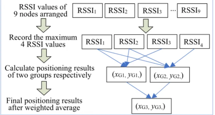
137
distance correction is constructed according to the median of distance deviation coefficient.
138
3.1. Basic concept
139
Definition 1. WSN node positioning. WSN node positioning refers that the position of the unknown target
140
node is calculated based on the communication between the anchor nodes whose position information are known
141
in the network by certain techniques, algorithms and schemes [30].
142
Definition 2. Anchor node. The anchor node is the node whose coordinates or position information is known in
143
WSN [31].
144
Definition 3. Target node. The target node refers to the node whose coordinates or positioning information is
145
unknown in the WSN [32].
146
3.2. The preprocessing of iterative positioning algorithm
147
Before the constructions of the iterative positioning algorithm, it is necessary to do some
148
preprocessing tasks. First of all, the mathematical model of RSSI was constructed and used to
149
calculate the initial measured distance. Then, analyzing the influence of noise on the measured
150
distance and constructing the noise impact factor. Finally, the triangle centroid positioning
151
algorithm is used to obtain the initial positioning coordinates of the target node.
152
3.2.1. RSSI ranging algorithm
153
The basic idea of the RSSI ranging algorithm is to calculate the distance between the
154
transmitting signal node and the receiving signal node by measuring the received signal strength
155
because there are varying degrees of losses in the propagation process of wireless signals. Therefore,
156
it is very important to build an appropriate RSSI ranging model. At present, the model used
157
commonly is the log-normal distribution model [33-35] .
158
Pd is used to indicate the power measurement corresponding to the distance between two
159
nodes as d, Pd
0is used to indicate the power measurement corresponding to the distance between
160
two nodes as d
0. The relationship between Pd and d can be expressed as
161
0
0 0
n
Pd Pd d
d
, (1)
where n is a signal propagation factor, which is usually obtained by empirical value or actual
162
calibration.
163
The logarithmic processing is performed on both sides of the formula (1), and after arranging,
164
the formula (2) can be obtained:
165
0
0
lg lg lg(d )
Pd Pd n
d
, (2)
And because the relationship between RSSI value and power can be expressed as:
166
10 lg
RSSI p
, (3)
Thus, a mathematical model of RSSI ranging can be obtained:
167
0
0
( ) ( ) 10 lg(d )
P d P d n
d
, (4)
where P(d) is the RSSI value when the distance between two nodes is d, and P(d
0) is the
168
RSSI value when the distance between two nodes is d
0.
169
3.2.2. The effect of noise on RSSI ranging
170
The loss of the wireless signal during propagation has a great influence on the accuracy of the
171
RSSI ranging algorithm and must be considered in practical applications. Next, we will analyze the
172
effect of signal propagation loss on RSSI ranging. In the formula (4), the measurement value P(d) is
173
composed of the true signal strength value and noise signal strength value, denoted as P
T(d) and P
N(d)
174
respectively. P(d
0) is the RSSI value when the distance between two nodes is d
0. To simplify the
175
calculation, d
0is usually taken as 1, and P(d
0) is denoted as A.
176
Thus, the actual mathematical model of the log-normal distribution model is as follows:
177
, (5)
From the formula (5), the distance between two nodes can be calculated as follows:
178
A ( ) ( )
=10
10T N
P d P d
d
n
, (6)
Equation (6) can be calculated as follows by further mathematical transformation:
179
( )
A ( )
10 10
=10 10
N
T P d
P d
n n
d
, (7)
Assume that
1A ( )
10 P dT
K n
,
2( ) 10 P dN
K n
.
180
Formula (7) can be expressed as
181
, (8)
Formula (8) can be expanded further as:
182
1 1 2
=10
K10 (10
K K1)
d , (9)
Assume that , Therefore, the calculation of distance d can be
183
simplified as follows:
184
=
T T Nd d d F , (10)
where d
T=10
K1is the true distance between the anchor node and the target node,
185
=10
K21
F
N is the impact factor of noise on distance measurement. F
Nis referred
186
to as noise impact factor in this paper.
187
3.2.3.The triangular centroid positioning algorithm
188
The basic principle of the triangle centroid positioning algorithm is as follows: the three circles
189
are determined by treating the three anchor nodes as their respective circle centres, by treating the
190
distances between the anchor nodes and the target node as their respective radiuses. The
191
intersection of the three circles can obtain six intersection points, a triangle is constructed by
192
treating the three closer intersection points as vertexes, the centroid of the triangle is taken as the
193
coordinates of the node to be positioned. The schematic diagram of triangular centroid positioning
194
is shown in Figure 2.
195
11 11
(x ,y )
33 33
(x ,y )
22 22
(x ,y ) O2
O3
O1 O
S
1S
2S
32 2
(x y, )
3 3
(x,y)
1 1
(x y, )
(xg,yg)
d
1d
2d
3196
Figure 2. Schematic diagram of triangular centroid positioning
197
In Fig. 2, and O
1, O
2and O
3are defined as the positions of three anchor nodes with coordinates
198
of O
1(x
11, y
11), O
2(x
22, y
22) and O
3(x
33, y
33), which radius are d
1, d
2, and d
3respectively. Point S
1(x
1, y
1),
199
S
2(x
2, y
2) and S
3(x
3, y
3) are the three closer intersections points, that is, the three vertices of the triangle
200
centroid positioning algorithm.
201
The intersection point coordinates of the circle O
1and the circle O
2can be obtained by equation
202
(11).
203
2 2 2
11 11 1
2 2 2
22 22 2
( ) ( )
( ) ( )
x x y y d
x x y y d
, (11)
In the 2 sets of coordinates solved by equation (11), the intersection S
3(x
3, y
3) closer to the
204
center of the positioning triangle. The solution of the remaining two points S
1(x
1, y
1) and S
2(x
2, y
2) is
205
similar to that of point S
3(x
3, y
3).
206
Thus, the initial coordinates O(x
g, y
g) of the target node can be calculated by equation (12).
207
= 1
= 1
1 1
m
g i
i m
g i
i
x x
m
y y
m
( m 3) , (12)
where m=3, i = 1, 2, 3.
208
3.3. The iterative positioning algorithm
209
In the actual physical environment, signals are easily disturbed by noise in the transmission
210
process. Therefore, there is a large deviation between the distance obtained by the log-normal
211
distribution model and the real distance value. In order to reduce the positioning error further, a
212
node iterative positioning algorithm based on distance correction is introduced in the paper.
213
The basic principle of the iterative positioning algorithm based on distance correction is as
214
follows: the distance deviation coefficient is introduced to evaluate the degree of deviation of the
215
measurement distance between the log-normal distribution model and based on the triangle
216
centroid positioning algorithm. The distance between the anchor node and the target node is
217
recalculated based on the distance deviation coefficient. By constantly updating the distance
218
between the anchor node and the target node, the target node coordinates are iteratively calculated.
219
3.3.1. The calculation of the distance deviation coefficient
220
The distance between the anchor node and the target node, which is calculated by the
221
log-normal distribution model, is denoted as d
biThe distance between the anchor node
222
coordinates and the coordinates, which are calculated by the triangle centroid positioning algorithm,
223
is denoted as d
ciIn order to indicate the deviation of the two distances, the distance deviation
224
coefficient C
devis defined as equation (13).
225
=
bidev ci
C d
d (i=1, 2, 3), (13)
Many distance deviation coefficients can be solved by the formula (13), and it is important to
226
determine a characteristic quantity to represent the degree of deviation of the overall node
227
measurement distance. The two statistical parameters, the average value and the median of distance
228
deviation coefficients, can both closely be used to express the overall distance deviation
229
characteristics.
230
The average value of distance deviation coefficients can be expressed the average level of the
231
overall measurement distance deviation. However, its fatal disadvantage is that if the extremum at
232
both ends is too low or too high, the final calculation result will greatly deviate from the real
233
situation.
234
Therefore, the median distance deviation coefficients are usually used to express the overall
235
distance deviation characteristic. The median is not affected by the extreme values of both ends, and
236
can better reflect the overall distance deviation characteristics, making the final calculation result
237
closer to the real situation.
238
The distance deviation coefficients are calculated by the formula (13), the median C
devcan
239
be obtained after sorting.
240
The distance between the anchor node and the target node can be recalculated based on the
241
median C
devas shown in equation (14).
242
=
bini dev
d d
C (i=1, 2, 3), (14)
The new distance d
niis obtained by the formula (14), and the triangular centroid positioning
243
algorithm is iteratively conducted to obtain the positioning result .
244
3.3.2. The iteration termination criteria for algorithm.
245
If the termination condition of the iterative positioning algorithm is set correctly, the higher
246
positioning accuracy can be obtained with only a small number of iterations, and the algorithm is
247
prevented from falling into an infinite loop. In general, the iteration termination condition is defined
248 249 as:
, (15)
Where is the RSSI value between the centroid of the nth iteration and the unknown target
250
node, ε is the set threshold.
251
Under different environmental conditions, if formula (15) is used as the iterative termination
252
condition, its computational complexity is very high, even higher than the complexity of the
253
iterative positioning algorithm itself. In this way, the hardware complexity of the system will
254
increase significantly and the algorithm become almost infeasible. In practical applications, as the
255
number of iterations increases, the positioning error has the following cases: fast convergence, slow
256
convergence, and periodic oscillation. By simulation analysis, it is found that,when the number of
257
iterations is between 0-10 times, the iteration error varies with different regular pattern,the
258
iteration error basically unchanged when the number of iterations is between 10-20 times.
259
The flow chart of the iterative positioning algorithm is shown in Figure 3.
260
261
Figure 3. The flow chart of the iterative positioning algorithm
262
4. The construction of iterative positioning model
263
In the procedure of iterative positioning, whether the target node is in the positioning triangle
264
area has great influence on its positioning accuracy. The positioning error of the target node located
265
in the positioning triangle area is much smaller than that of the target node outside the positioning
266
triangle area. In order to improve the positioning accuracy, an iterative positioning model is
267
established in the paper, as shown in Figure 4.
268
269
Figure 4. A schematic of the positioning model
270
In Figure 4, the quadrilateral A
1A
2A
3A
4is a square, the point O is its center, the points B
1, B
2, B
3271
and B
4are the midpoints of the respective sides. According to the connection shown in Figure 4, the
272
square A
1A
2A
3A
4is subdivided into eight triangular regions: region 1 to region 8. The anchor nodes
273
(9 in total) are placed at points A
1, A
2, A
3, A
4, B
1, B
2, B
3, B
4and O.
274
There is a target node X in the quadrilateral A
1B
1OB
4in Figure 4, the points closest to the point X
275
are points A
1, B
1, O, B
4in turn. The node X is included in both △A
1B
1B
4and △A
1B
1O. In the △A
1B
1B
4,
276
Calculating the distance dbi
between anchor node and target node
Obtaining the initial positioning coordinates Conducting the triangular centroid algorithm positioning
Calculating distance deviation coefficient Cdev
Initialization iterations
Output iterative positioning results
Y N
Getting the median after arranging
Recalculating the distance dni between anchor node and target node
Conducting again the triangular centroid algorithm positioning
Obtaining the iterative positioning coordinates (xG, yG)
Reaches the number of iterations?
the coordinates (x
G1, y
G1) is calculated by iterative positioning algorithm. In order to reduce
277
effectively the positioning error caused by noise, the other coordinate is calculated by
278
the iterative positioning algorithm in △A
1B
1O. The weighted average of these two coordinates can be
279
taken as the final coordinates . Obviously, the closer the distance between the anchor
280
node and the target node is, the more reliable the calculation result is. Hence the weight of the
281
former coordinate should be greater than the weight of the latter coordinate.
282
The various proportion of weight value are compared by the simulation experiment, the results
283
show that when the weight of the former coordinate is 0.75 and the weight of the latter coordinate is
284
0.25, the positioning result better than others.
285
The final positioning results can be expressed as follows in equation (16).
286
2 1
3
2 1
3
25 . 0 75 . 0
25 . 0 75 . 0
G G
G
G G
G
y y
y
x x
x , (16)
In actual positioning progress, the RSSI values of the 9 anchor nodes are recorded and arranged
287
in descending order of their values. The first four larger RSSI values are denoted as RSSI
1, RSSI
2,
288
RSSI
3and RSSI
4. The first positioning coordinates (x
G1,y
G1) is calculated by RSSI
1, RSSI
2, RSSI
3and
289
their corresponding coordinates. The second positioning coordinates (x
G2,y
G2) is calculated by RSSI
1,
290
RSSI
2and RSSI
4and their corresponding coordinates. The weighted average of two coordinates
291
according to the weights mentioned above is the final positioning result (x
G3,y
G3).
292
The positioning process of the iterative positioning algorithm is shown in Figure 5:
293
294
Figure 5. The specific implementation process of iterative positioning
295
5. Experiment
296
5.1. The experimental method
297
In order to verify the performance of the algorithm proposed in the paper accurately and
298
quantitatively, without loss of generality, the positioning experimental area is set as a square of
299
40m*40m. There are nine anchor nodes in the positioning experimental area, which are located at
300
the vertices of the square, the middle of each edge and the center of the square. Now, 50 target
301
nodes are generated in the square area by random, and calculating their positioning results in turn.
302
In the experiment, for different noise impact factors F
N, positioning error is discussed by three
303
methods of the centroid positioning algorithm, the weighted centroid positioning algorithm and the
304
iterative positioning algorithm based on distance correction. The value of F
Nis taken into account in
305
two situations: constant value and random value.
306
5.2. Experimental analysis
307
According to the above experimental method, two experiments have been conducted.
308
5.2.1. The first experiment: F
Nis constant
309
When F
Nis a constant value, considering the effects of the actual noise on the signal, three
310
RSSI values of ...
9 nodes arranged RSSI1 RSSI2 RSSI3 RSSI9
RSSI1 RSSI2 RSSI3 RSSI4 Record the maximum
4 RSSI values
Calculate positioning results of two groups respectively
Final positioning results after weighted average
(xG1, yG1,) (xG2, yG2,)
(xG3, yG3,)
typical F
Nvalues are taken for experiments, which are 0.1, 0.2 and 0.3 respectively.
311
The experiments for three parameters are shown as follows:
312
● F
N=0.1
313
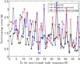
The positioning error is shown as Figure 6 in the case of the noise impact factor of 0.1.
314
315
Figure 6. The positioning error of the three positioning algorithms in the case of the noise impact
316
factor of 0.1
317
The x-coordinate represents the target node sequence, the unit is the number of nodes. The
318
y-coordinate represents the positioning error, the unit is meter.
319
● F
N=0.2
320
The positioning error is shown as Figure 7 in the case of the noise impact factor of 0.2.
321
322
Figure 7. The positioning error of the three positioning algorithms in the case of the noise impact
323
factor of 0.2
324
● F
N=0.3
325
The positioning error is shown as Figure 8 in the case of noise impact factor of 0.3.
326
327
Figure 8. The positioning error of the three positioning algorithms in the case of noise impact factor
328
of 0.3
329
5.2.2. The second experiment: FN is a random value
330
When F
Nis a random value, considering the effect of the actual noise on the signal, the random
331
value is 0.3 times of random function.
332
The positioning error is shown as Figure 9 in the case of the noise impact factor of random
333
value.
334
0 5 10 15 20 25 30 35 40 45 50
0 0.5 1 1.5 2 2.5 3 3.5
335
Figure 9. The positioning error of the three positioning algorithms in the case of the noise impact
336
factor of random value
337
In the case of different noise impact factors, the positioning errors of the three positioning
338
algorithms are shown in Table 1.
339
Table 1. The positioning error of the three positioning algorithms in the case of different noise impact
340
factors
341
Noise impact factor Average positioning error (m)
Centroid Weighted centroid Iterative positioning
F
N=0.1 0.77 0.70 0.17
F
N=0.2 1.68 1.30 0.32
F
N=0.3 2.63 1.85 0.59
F
N=random 1.75 1.53 1.09
As can be seen from Table 1, when FN is a random value, the positioning accuracy of the
342
iterative positioning algorithm is improved by 38% compared with the centroid algorithm, and the
343
positioning accuracy of the iterative positioning algorithm is improved by 29% by comparing with
344
the weighted centroid algorithm.
345
The positioning error of the three positioning algorithms for different values of noise impact
346
factors is shown in Figure 10.
347
0 0.5 1 1.5 2 2.5 3
0.1 0.2 0.3 Random value
Noise impact factor value
Averagepositioningerror(m)
Centroid Weighted centroid Iteration
348
Figure 10. The positioning error of the three positioning algorithms under different noise influence
349
factors
350
As can be seen from Figure 10, the positioning error of the iterative positioning algorithm is
351
smaller than that of the centroid positioning algorithm and the weighted centroid positioning
352
algorithm in the case of different noise impact factors F
N.
353
6. Conclusions
354
With the development of wireless communication technology, the position information of data
355
is playing an increasingly important role. There are errors in node positioning due to various
356
interferences in the data transmission process. To solve this problem, a node iterative positioning
357
algorithm based on distance correction is proposed in this paper to help users obtain accurate
358
position information. Contributions include the following aspects.
359
(1) The noise impact factor FN has been derived on the basis of the original log-distance
360
distribution model, which is used to describe the corresponding relationship between the noise
361
impact factor FN and the measured distance. Proposing of noise impact factor provides a novel
362
method for analyzing the influence of noise on the distance measurement between nodes in WSN.
363
(2) The median of the distance deviation coefficient has been constructed to characterize the
364
deviation degree of the whole measured distances, and used to correct the distance from the last
365
positioning. The triangle centroid localization algorithm has been iteratively conducted based on the
366
corrected new distance value to improve the node positioning accuracy.
367
The experimental results show that the node iterative positioning algorithm based on distance
368
correction can effectively reduce the positioning error of unknown target nodes in wireless sensor
369
networks, and help users obtain more accurate node coordinates. In the future, based on the node
370
iterative positioning algorithm proposed in the paper, we will do some related researches such as
371
real-time tracking and path planning of moving nodes in WSN.
372
Author Contributions: Conceptualization, J.C., S.W., and M.O.; Methodology, all authors; Software, J.C. M.O.,
373
and Y.C.; Validation, J.C and Y.X.; Formal Analysis, J.C., S.W., and Y.X.; Investigation, J.C, and M.O.; Resources,
374
J.C., S.W. and Y.C.; Data curation, S.W.,Y.C. and Y.X.; Writing—Original Draft Preparation, J.C. and M.O.;
375
Writing—Review & Editing, J.C., S.W., and M.O.; Visualization, J.C. and Y.C.; Supervision, J.C. and M.O.;
376
Project administration, J.C. and M.O.; Funding acquisition, J.C.
377
Funding: This research was funded by Natural Science Fundation of Education Department of Anhui province
378
(KJ2018A0087) and Natural Science Foundation of China (51874010).
379
Conflicts of Interest: The authors declare no conflict of interest.
380
References
381
1. S. Pandey, S. Varma. A Range-Based Localization System in Multihop Wireless Sensor Networks A
382
Distributed Cooperative Approach. Wireless Personal Communications 2016, 86, 615-634. [ DOI:
383
10.1007/s11277-015-2948-3]
384
2. S. Safavi, U. A. Khan. Localization in mobile networks via virtual convex hulls. IEEE Transactions on Signal
385
and Information Processing over Networks 2018, 4, 188-201. [DOI: 10.1109/TSIPN.2017.2673238]
386
3. M. A. Benatia, M. Sahnoun, D. Baudry, A. Louis, A. El-Hami, B. Mazari. Multi-Objective WSN
387
Deployment Using Genetic Algorithms Under Cost, Coverage, and Connectivity Constraints. Wireless
388
Personal Communications 2017, 94, 2739-2768. [doi.org/10.1007/s11277-017-3974-0]
389
4. M.R. Senouci and H.E. Lehtihet. Sampling-based selection-decimation deployment approach for
390
large-scale wireless sensor networks. Ad Hoc Networks 2018, 75-76, 135-146.
391
[DOI: 10.1016/j.adhoc.2018.04.002]
392
5. P. Raja1, P. Dananjayan. Game Theory Based Cooperative MIMO Routing Scheme for Lifetime
393
Enhancement of WSN. International Journal of Wireless Information Networks 2015, 22, 116-125. [DOI
394
10.1007/s10776-015-0268-x]
395
6. R. Rai, P. Rai. Survey on Energy-Efficient Routing Protocols in Wireless Sensor Networks Using Game
396
Theory. Advances in Communication, Cloud, and Big Data 2019, 31, 1-9. [DOI: 10.1007/978-981-10-8911-4_1]
397
7. S. Halder1, A. Ghosal1. A survey on mobile anchor assisted localization techniques in wireless sensor
398
networks. Wireless Networks 2016, 22, 317-2336. [DOI: 10.1109/COMST.2016.2544751]
399
8. Alletto S, Cucchiara R, Fiore G D, et al. An Indoor Location-Aware System for an IoT-Based Smart
400
Museum. IEEE Internet of Things Journal 2016, 3, 244-253. [DOI: 10.1109/JIOT.2015.2506258]
401
9. ZHANG X. R, XIONG W. L, XU B. G. A Whole Process Optimization Distributed Localization Strategy
402
Based on RSSI in Wireless Sensor Networks. Chinese Journal of Sensors and Actuators 2016, 29, 1875-1881.
403
10. Tomic S, Beko M, Rui D. Distributed RSS-AoA Based Localization with Unknown Transmit Powers[J].
404
IEEE Wireless Communications Letters 2016, 29, 3-395. [DOI: 10.1109/LWC.2016.2567394]
405
11. P. K. Sahu, E. H.-K. Wu, and J. Sahoo. DuRT: Dual RSSI Trend Based Localization for Wireless Sensor
406
Networks. IEEE Sensors Journal 2013, 13, 3115-3123. [DOI: 10.1109/JSEN.2013.2257731]
407
12. F. Yaghoubi, A.-A. Abbasfar, and B. Maham. Energy-efcient RSSI-based localization for wireless sensor
408
networks. IEEE Communications Letters 2014, 8, 973-976. [DOI: 10.1109/LCOMM.2014.2320939]
409
13. S. Tomic, M. Beko, and R. Dinis. RSS-based localization in wireless sensor networks using convex
410
relaxation: on cooperative and cooperative schemes. IEEE Transactions on Vehicular Technology 2015, 64,
411
2037-2050. [DOI: 10.1109/TVT.2014.2334397]
412
14. Y. Hou, X. Yang, and Q.H. Abbasi. Efficient AoA-Based Wireless Indoor Localization for Hospital
413
Outpatients Using Mobile Devices. Sensors 2018, 18 3698. [Doi.org/10.3390/s18113698]
414
15. X. H. Zhang, T. J. Wang, J. L. Fang. A node localization approach based on mobile beacon using particle
415
swarm optimization in wireless sensor networks. International Journal of Embedded Systems 2017, 9, 112-118.
416
[https://doi.org/10.1504/IJES.2017.083731]
417
16. C. Ke, M. Wu, Y. Chan, K. Lu. Developing a BLE Beacon-Based Location System Using Location
418
Fingerprint Positioning for Smart Home Power Management. ENERGIES 2018, 11, 3464.
419
[doi.org/10.3390/en11123464]
420
17. T. J. S. Chowdhury, C. Elkin, V. Devabhaktuni, D. B. Rawat, and J. Oluoch. Advances on localization
421
techniques for wireless sensor networks: A survey. Computer Networks 2016, 110, 284-305.
422
[doi.org/10.1016/j.comnet.2016.10.006]
423
18. Z. Wang, H. Zhang, T. Lu, T. A. Gulliver. Cooperative RSS-Based localization in wireless sensor networks
424
using relative error estimation and semidefinite programming. IEEE TRANSACTIONS ON VEHICULAR
425
TECHNOLOGY 2019, 8, 483-497. [DOI: 10.1109/TVT.2018.2880991]
426
19. G. Sharma, A. Kumar. Improved range-free localization for three-dimensional wireless sensor networks
427
using genetic algorithm. Computers & Electrical Engineering 2018, 72, 808-827.
428
[doi.org/10.1016/j.compeleceng.2017.12.036]
429
20. Zhang Y, Xu X. L, Xu K. Y. Algorithm based on weighted centroid method for WLAN indoor positioning.
430
Journal of Electronic Measurement and Instruments 2015, 29, 1036-1041.
431
21. S. Phoemphon, C. So-In, N. Leelathakul. Fuzzy Weighted Centroid Localization with Virtual Node
432
Approximation in Wireless Sensor Networks. IEEE Internet of Things Journal 2018, 5, 4728-4752. [DOI:
433
10.1109/JIOT.2018.2811741]
434
22. S. B. Shah, Z. Chen, F. Yin, I. U. Khan, S. Begum, M. Faheem, F. A. Khan. 3D weighted centroid algorithm
435
& RSSI ranging model strategy for node localization in WSN based on smart devices. Sustainable Cities and
436
Society 2018, 39,298-308 [doi.org/10.1016/j.scs.2018.02.022]
437
23. H. Huo, H.H. Yang, D.Y. Zhen, L. Liu, W. Zhang. Advanced indoor position algorithm based on RSSI
438
fingerprint. Application Research of Computers 2017, 24, 2786-2790.
439
24. X. Fang, Z. Jiang, L. Nan, L. Chen. Optimal weighted K-nearest neighbour algorithm for wireless sensor
440
network fingerprint localisation in noisy environment. IET COMMUNICATIONS 2018, 12, 1171-1177.
441
[DOI: 10.1049/iet-com.2017.0515]
442
25. C. Panarat, S. Pitikhate. Soft-clustering Technique for Fingerprint-based Localization. SENSORS AND
443
MATERIALS 2018, 30, 2221-2233. [doi.org/10.18494/SAM.2018.1844]
444
26. M. Gholami, N. Cai, R. W. Brennan. An artificial neural network approach to the problem of wireless
445
sensors network localization. Robotics and Computer-Integrated Manufacturing 2013, 29, 96-109.
446
[doi.org/10.1016/j.rcim.2012.07.006]
447
27. B. S. Saber, A. Fazlollah, S. Mehdi A. A New Range-Free and Storage-Efficient Localization Algorithm
448
Using Neural Networks in Wireless Sensor Networks. Wireless Personal Communications 2018, 98,
449
1547-1568. [Doi:10.1007/s11277-017-4934-4]
450
28. Sun X, Yao H, Zhang S, et al. Non-Rigid Object Contour Tracking via a Novel Supervised Level Set Model.
451
IEEE Transactions on Image Processing 2015, 24, 3386-3399. [DOI: 10.1109/TIP.2015.2447213]
452
29. K. G. Qian, Y. J. Wang, X. M. Li, Z. C.Dai. An Improved Bounding Box Localization Algorithm Based on
453
Optimum Node Selection. Applied Mechanics and Materials 2014, 668-669, 1359-1362.
454
[doi.org/10.4028/www.scientific.net/AMM.668-669.1359]
455
30. S. Saunhita, M. S. Optimized Relay Nodes Positioning to Achieve Full Connectivity in Wireless Sensor
456
Networks. WIRELESS PERSONAL COMMUNICATIONS 2018, 99, 1521-1540.
457
[Doi:10.1007/s11277-018-5290-8]
458
31. P. Singh, A. Khosla, M. Khosla, A. Kumar. Computational intelligence based localization of moving target
459
nodes using single anchor node in wireless sensor networks. Telecommunication Systems 2018, 69, 397-411.
460
[doi:10.1007/s11235-018-0444-2]
461
32. P. Singh, A. Khosla, A. Kumar, M. Khosla. Optimized localization of target nodes using single mobile
462
anchor node in wireless sensor network. International Journal of Electronics and Communications 2018, 91,
463
55-65. [DOI: 10.1109/IC3TSN.2017.8284493]
464
33. E. Goldoni, A. Savioli, M. Risi, and P. Gamba. Experimental analysis of RSSI-based indoor localization
465
with IEEE 802.15.4. IEEE Proc. of European Wireless Conference 2010, 71-77. [DOI: 10.1109/EW.2010.5483396]
466
34. TIAN Z. J, LI Z. W, LIU X. Y, et al. A Positioning Method in Mine Tunnel Based on Joint Electromagnetic
467
Wave and Ultrasonic Distance Measurement. Transactions of Beijing Institute of Technology 2014, 34,
468
1177-1185.
469
35. Zheng X. L, Fu J. Q. Research on Indoor Location Algorithm Based on PDR and RSSI’, Journal of
470
Instrumentation 2015, 36, 1177-1185.
471