Modeling for Operating Expenses and Time Consumption of High Speed Railway (HSR)

Modeling for Operating Expenses and

Time Consumption of High-Speed

Railway (HSR)

Noor, Bashar Abdal and Sirong, Yi and Alam Kazmi, Syed

Hasnain and Abid, Malik Muneeb

Southwest Jiaotong University

10 August 2016

Mod

Basha

In the l

Recent

deling fo

ar Abdal

1_Department 2_{School o} 3_{School of Tr}

ct

ortation plays c harmonious g vertical prof spacing on ption. In this show that op ption model

has great imp

ds: operating

Introductio

ast decade,

HSR infras

or Oper

Hi

Noor

, Yi

t of Road and of Economics ransportation a

a significant s developmen file of high-sp operating exp regard, six s perating expe is a quadratic pact on operati

expenses, tim

on

the world h

structure is

rating E

igh-Spe

i Sirong

,

Railway Engi and Managem and Logistics,

(malik.m

t role in each nt. Operating peed railway l

penses, and i standard verti enses model c function of ing expenses a me consumptio has cherish the result

Expense

eed Rail

Syed Ha

Abid

ineering, Sout ment, Southwe , Southwest Ji muneeb.abid@

h country’s ec expenses an ine. The pape ii) second m ical profiles o

is a third-d f maximum g and time cons on, high-speed

ed the rapid

of specializ

es and T

lway

(

H

snain Ala

3

thwest Jiaoton est JiaoTong U iaoTong Univ @hotmail.com)

conomy and nd time consu er presents two measures the e of high-speed degree functio gradient. Furth sumption of H d railway, vert

d developm zed develop

Time Co

HSR)

am Kazmi

it is critically umption are o models: i) fi effect of max d railway line

on of station hermore, it is HSR.

tical profile, st

ment of high

pment techn

onsump

i

, Malik

, Chengdu, Ch hengdu, China du, China 610

y important to important in irst estimates ximum gradie e have been s n spacing, wh

s determined

tation spacing

h-speed railw

niques in th

ption of

k Muneeb

hina. a. 0031.

which results into the expanded the passenger traffic system (Gong, 2010). The passenger

high-speed train operates significantly faster (300 km/h) than the normal high-speed (120 km/h) of rail

traffic and has great attraction for passengers (International Union of Railways, 2015). The

European Union pays a special consideration for the railway transport development to minimize

the undesirable (traffic jams, damage to the environment, noise, accidents) influence of

dominating factors in transportation network (Vytautas and Gintaras, 2014). According to the

definitions of the European Union, high-speed railway refers to the transformed railway tracks

whose operating speed should be 200 km/h or more and the new specialized railway tracks

whose operating speed can be 250 km/h or more (International Union of Railways, 2015). The

social and economic benefits are one of the important attributes of high-speed railways beside

many others like, high-speed, large passing capacity, high efficiency and less pollution. Many

studies on efficient energy management have been carried out in metro and rail transit systems

(Ennio and Pierluigi, 2014; Ashiya and Yasuda, 1994). The reduction of energy consumption is

also seen as one of the key objectives for the development of sustainable mobility by use of

HSR. The completion of a HSR project will lead to a huge increase in electricity consumption in

spite of the comparatively lower mean energy consumption per passenger kilometer for normal

train (High-Level Group, 1995). Moreover, a HSR project requires a very heavy investment for a

country mainly due to the cost of civil works. Therefore, high investment must be balanced by a

shorter trip time and lower energy consumption.

In recent years, more than ten countries in the world have built HSR, including Spain, Japan,

Germany, France, China, and the United States (International Union of Railways, 2015/UIC).

HSR from many views, such as infrastructure, rolling stock and operations. Nevertheless, HSR is

a combination of all the elements that constitute the “system” (Aurélie 2011):

1. Infrastructure: new dedicated lines designed for speeds above 250 km/h; upgraded normal

lines, which enable trains to operate up to 200 or even 220 km/h.

2. Rolling stock and operating conditions: special trains that differ from normal rolling stock

with an increased power/weight ratio and several characteristics such as aerodynamics,

reliability, safety.

Due to the constraints in train routes and other economic and technical reasons, high-speed trains

cannot provide the “door to door” service for passenger, so that the passenger distribution of

speed railway station must be completed by means of urban traffic system. Thus,

high-speed railway station is also one joint point between urban external communication and intra-city

traffic system, where is the change place of traffic modes and transport properties. The aim of

high-speed railway station location is to control trip time of passengers, and reduce the pressure

of urban road traffic network and improve transportation energy efficiency (Xiang et al., 2010).

In this context a technique for calculation of time consumption and operating expenses, derived

by Wang D. and Wang D.S. (2000), is in the form of mathematical models and graphs. They

expected that the theoretical idea and the main procedures could be applied for HSR. Their work

was done in cooperation with engineers of the Third Design Institute of Chinese Railway

Ministry and was proved satisfactory in practical designs for normal speed railways. By referring

to several vertical profiles of railway lines, Wang D. and Wang D.S. (2000) have also suggested

six standard vertical profiles between passing sidings or intermediate stops. In this paper, the

authors have applied their technique to HSR. It is concluded that when station spacing is small

and vice versa.

2. Literature Review

like travel speed, passing capacity and transportation organizational modes. He found that setting the stations in full accordance with the needs of passenger traffic will worsen the passing capacity, the number of running train and travel speed that will caused in more time consumption.

Zeng et al. (2013) introduced variable of comfort levels to calculate the generalized value of travel time. A pricing model, which is based on the value of travel time and bi-level programming, presented to maximize the benefit of the railway agencies and the passengers’ utility. Model considered the passenger’s mode choice behavior with different income levels. They found that using the model by actual survey and pricing is more acceptable compared with the pricing method in the current condition. Through the actual investigation, the price got by model based on value of travel time and bi-level programming was more reasonable than the existing price. Travel time reliability is a fundamental factor in travel behavior. It represents the temporal uncertainty experienced by travelers in their movement between any two nodes in a network. The importance of the time reliability depends on the penalties incurred by the travelers. Carrion and Levinson (2012) presented a systematic review of the current state of research in travel time reliability, and more explicitly in the value of travel time reliability. To increase the overall benefits of the HST (and decrease its negative effects), it should serve many cities and include many stops, but more stations on an HST line lead to a lower average speed and thus to lower capacity on the route and a longer travel time (Hang, 2011). Recently, Abid and Khan (2015) proposed a MILP model to find the position of stations with sidings on the railway network to minimize the conflict delays.

Various researchers present different social and economic effects of transport projects (Lingaitis, 2009; Robert and Daniel, 2012). Summarizing the authors’ suggestions, the passenger transport system’s modernization effects can be grouped into the effects of transport systems changes and the effects of social economic changes that measure the interests of passengers, transport companies, regions and countries. The evaluation indicators proposed the following points: the change of travelling time, the changes of technological costs of passenger transport, the changes of traffic and ecological safety, the changes of comfort level, and the changes of a company’s cohesion and economic development. According to the experts, one of the most important indicators of passenger transport's economic social efficiency is the value of travel timesaving. 30 to 80 percent of the overall transport project benefit is thought to come from the reduced traveling time during which a passenger does not participate in the formation process of added value (Vytautas and Gintaras, 2014).

3. Research Methodology

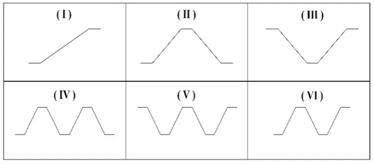
planning and design stages but also useful for examining the efficiency of existing railways (Yi and He, 2009). In the framework, a method for the calculation of operating expenses and time consumption are derived from Wang and Wang (2000) in the form of mathematical models and graphs. By comparing the large volume of design data, authors found that the vertical profiles between passing sidings or intermediate stops could be classified into six types of simulated designs, mentioned as vertical profiles I, II, III, IV, V and VI (see Figure 1).

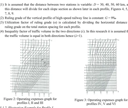
Operating expenses modeling has implemented the earlier discussed methodology of normal speed railway for modeling operating expense (E) to high-speed railways. Figure 2 shows the graph for calculating operating expenses of profiles I, II and III. Figure 3 shows the graph for calculating operating expenses of profiles IV, V and VI. Time Consumption Modeling has also adopted a methodology that implies using previously mentioned six types of vertical profiles. We have calculated the maximum gradient values with different maximum speed on HSR, besides getting the value of time consumption.

Figure 1: Six types of vertical profiles of high-speed railway Table 1: Table of Notation

D Station spacing (km)

λ Inequality factor of traffic volume in the

E Operating expenses (¥)

¥ RMB (Chinese Currency)

G Ruling grade ‰

α Factor of utilization of ruling grade

R2 coefficient of determination

f (D) Function of station spacing

imax Maximum gradient of slope (‰)

Pk Required power per ton (kW/t)

Vmax Maximum speed of train (km/h).

g Gravity acceleration (g = 10 m/s2).

W0 Basic resistance of maximum speed of running

/ Time consumption of train running between station ts Extra time consumption for starting a train (min)

tp Extra time consumption for parking a train (min)

Li Horizontal length of slope (km)

ti Time consumption per kilometer for a train on a

Vi Balancing speed (km/h)

D Braking distance (m)

V Speed of the train (km/h)

a Deceleration of the train(m/s2)

t Time consumption (min)

3.1 Operating Expenses Modeling

3.1.1 Assumptions for study

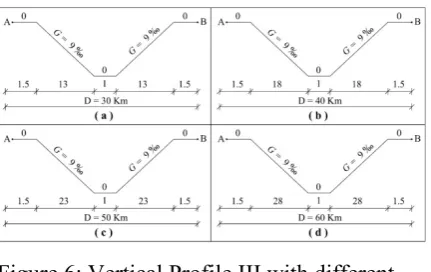
(1) It is assumed that the distance between two stations is variable: D = 30, 40, 50, 60 km, and this distance will divide for each slope section as shown later in each profile, Figures 4, 5, 6, 7, 8, 9.

(2) Ruling grade of the vertical profile of high-speed railway line is constant: G = 9‰

(3) Utilization factor of ruling grade (α) is calculated by dividing the horizontal distance of ruling grade on the total station spacing for each profile.

(4) Inequality factor of traffic volume in the two directions (λ). In this research it is assumed that the traffic volume is equal in both directions hence (λ=1).

Figure 2: Operating expenses graph for

profiles I, II and III Figure 3: Operating expenses graph for _{profiles IV, V and VI}

3.1.2. Illustration Example for Profile I

Figure 4: Vertical Profile I with different station spacing

Figure 5: Vertical Profile II with different station spacing

Figure 6: Vertical Profile III with different station spacing

Figure 7: Vertical Profile IV with different station spacing

Figure 8: Vertical Profile V with different station spacing

Figure 9: Vertical Profile VI with different station spacing

3.2 Time Consumption Modeling

The maximum gradient of slope (imax) is calculated by using formula (1), (Yi 2008; Yi and He

2009):

  . . .

.     ‰ (1)

Where, Pk: required power per ton (kW/t)

Vmax: Maximum speed of train (km/h)

g: Gravity acceleration (g = 10 m/s2)

w0: Basic resistance of maximum speed of running train (N/kN)

For calculating basic resistance for China Railway High-speed (CRH) Electrical Motor train Unit (EMU), this research will use formula (2) by (Yi 2008; Yi and He 2009):

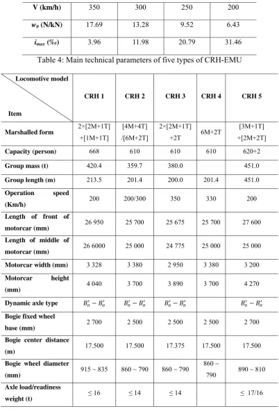
0.66 0.00245 0.000132 (2) Table 3 shows the values of maximum gradient of the vertical profile of HSR when maximum speed of CRH3 (EMU) is varying from 350 km/h to 200 km/h.

3.2.2. Time Consumption

Time consumption of train running between station A and station B is calculated by using formula (3), (Yi 2008; Yi and He 2009).

_/ ∑ ∙ (min) (3) Where: ts, tp: Extra time consumption for starting and parking a train. In general, for electric

traction and diesel traction: ts = 1~ 3 min; tp= 1~ 2 min.

Li: Horizontal length of slope (km)

ti: Time consumption per kilometer for a train on a slope section (min/km), for ascending

train, ti= 60 / Vi where Vi is the balancing speed and can be calculated from unit force graph. But

as the braking system of high speed train is activated by using computer-controlled comprehensive braking mode, and it doesn’t has the concept of train converted braking ratio and brake lining converted friction coefficient which is in general referred as train brake calculation, and also doesn’t need to consider the train basic resistance and gradient resistance, so the effective braking distance can be directly calculated by a given deceleration, (Zhang and Ma 2006). When the train is getting off a slope, ti is calculated from the formula (4):

. (4) Where, D: Braking distance (m)

Vmax: Maximum speed of the train (km/h)

t: Time consumption (min)

However, when the train is getting off a slope and there is a station at the end of the gradient section, the running time is calculated according to formula (5) of uniformly variable motion:

.   . (5)

Where, D: Braking distance (m) V: Speed of the train (km/h) a: Deceleration of the train (m/s2) t: Time consumption (min)

1- It is assumed that the distance between two following stations is constant (L = 30 km) and this distance will divide for each gradient section as shown later in each profile, (Figures 4-a, 5-a, 6-a, 7-6-a, 8-6-a, 9-a).

2- The additional time for starting and parking of the train is considered to be 3 min:

3 min.

3- This research chooses the CRH – EMU type-3 and Figure 14 shows its unit force curve, (Yi 2008).

Table 4 shows main technical parameters of five types of China Railway High-speed (CRH) Electrical Motor train Unit (EMU), (Yi and He 2009). From main technical parameters of CRH3 – EMU (Table 4): Pk = 21.05 kW/t , Vmax = 350 km/h. Figure 14, shows Unit force curve of

CRH3 – EMU

3.2.4 Illustration of Calculation Process for Profile I

When high-speed train pass through an area imitated as profile I between station A and station B, time consumption is calculated by using the formula (3):

  ∑ .

_⁄   . . .  

As shown in profile I (Figure 4-a) and by using first value of maximum gradient (Table 3):

i1 = i3= 0, i2 = imax = 3.96 ‰

From unit force curve of CRH3 – EMU (Figure 14), associated speed value of CRH3-EMU for each gradient is as follow: 341.44  / , 340.69  /

Now, by replacing in formula (3):

_⁄  

. 1.5 . 27 . 1.5  3 8.28 

By repeating previous calculation for all values of maximum gradient (Table 3) and drawing the graph, this research is getting time consumption model for each profile as shown later.

4. Computational Experiments

This section presents the application of the proposed methodologies with real world case study of HSR from Guiyang – Guangzhou China.

4.1 Case Study

economic development along the line is of great meaning for implementation of the western development strategy and sustainable development and construction of harmonious society.

4.2 Results

4.2.1Operating Expenses

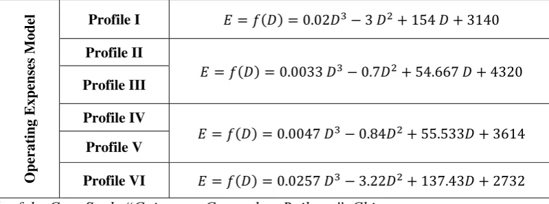
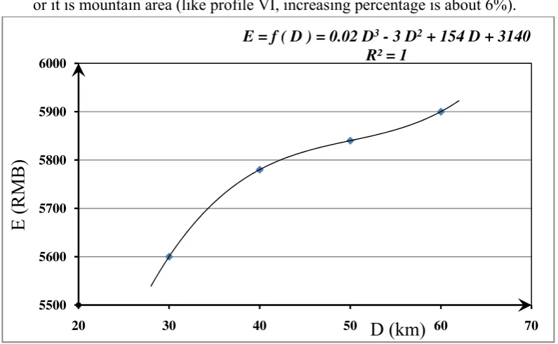
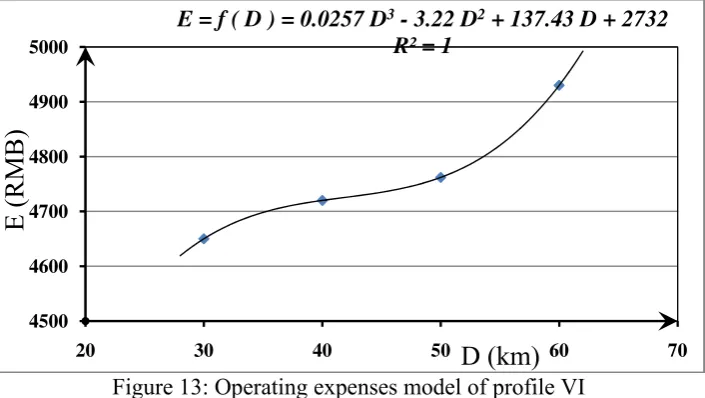
Figures 10, 11, 12, and 13 shows the relationship between operating expenses value and station spacing for profiles I, II/III, IV/V, and VI respectively. Table 1 shows operating expenses model for each standard vertical profile. Based on the implicit analysis mentioned earlier, the following results are established.

(1) Operating expenses model is a third-degree function for all profiles. The R-square values for all models are equal to one, as shown in the figures 10, 11, 12, 13.

(2) The results show that operating expenses are similar for the profiles, which have symmetrical sketch with a horizontal axis, whereas unsymmetrical sketch of different profiles have different values of operating expenses.

(3) Both profiles II and III have equal values of operating expenses, consequently they have the same model of operating expenses; additionally the profile IV and V accept the same effect.

(4) Operating expenses upsurges with the increasing of station spacing for each profile. (5) The percentage of increasing of operating expenses between the first and the last value of

station spacing for each profile is 5.36% for profile I, 7% for profiles II and III, 6% for profiles IV and V and it is 6% for profile VI.

Table 1. Operating expenses model for six standard vertical profiles of high-speed railway

Operating E x p en se s M odel

Profile I 0.02 3 154 3140

Profile II

0.0033 0.7 54.667  4320

Profile III

Profile IV

0.0047 0.84 55.533 3614

Profile V

Profile VI 0.0257 3.22 137.43 2732

Result of the Case Study “Guiyang – Guangzhou Railway”, China

Theoretical study has applied to few sections of case study railway line. Table 2 shows the operating expenses for stations spacing of the case study (Guiyang – Guangzhou) according to the sixth profiles. From Table 2, the following results are established:

Table 2. Operating expenses values for stations spacing of case study

LingTian–NanYu

D = 31.8 km 5646.63 5456.66 4681.65 4672.53

NanYu–GongCheng

D = 47.56 km 5829.95 5691.60 4860.72 4749.45

GongCheng–Lian’an

D =37.57 km 5751.87 5560.78 4763.95 4713.08

Lian’an–West ZhonShan D =21.44 km

5259.85 5202.81 4464.82 4451.63

West ZhonShan– Hezhou D =24.45 km

5404.22 5286.38 4538.32 4542.88

(1) The smallest station spacing is 21.44 km between (Lian’an – West Zhongshan), and when the vertical profile is shifting from plain area (like profile I) to a mountain area (like profile VI), the operating expenses will decrease about 15%.

(2) The largest station spacing is 47.56 km between (Nanyu – Gongcheng), and when the vertical profile is shifting from plain area (like profile I) to a mountain area (like profile VI), the operating expenses will decrease about 18%.

(3) When the station spacing is increasing from the smallest one (Lian’an – West Zhongshan) to the biggest area, (Nanyu – Gongcheng), the operating expenses is also increasing whether it is plain area (like profile I, increasing percentage is about 10%) or it is mountain area (like profile VI, increasing percentage is about 6%).

Figure 10: Operating expenses model of profile I

E = f ( D ) = 0.02 D3_{- 3 D}2_{+ 154 D + 3140}

R² = 1

5500 5600 5700 5800 5900 6000

20 30 40 50

_{D (km)}

Figure 11: Operating expenses model of profile II/III

Figure 12: Operating expenses model of profile IV/V

E = f ( D ) = 0.0033 D3_{- 0.7 D}2_{+ 54.667 D + 4320}

R² = 1

5300 5400 5500 5600 5700 5800 5900

20 30 40 50 60 70

D (km)

E (RMB)

E = f ( D ) = 0.0047 D3_{- 0.84 D}2_{+ 55.533 D + 3614}

R² = 1

4500 4600 4700 4800 4900 5000

20 30 40 50 60 70

E (RMB)

Figure 13: Operating expenses model of profile VI

4.2.2 Time Consumption

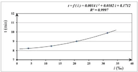
Figures 15, 16, 17 and 18 show the relationship between time consumption and maximum gradient for profiles I, II/III, IV/V, and VI respectively.

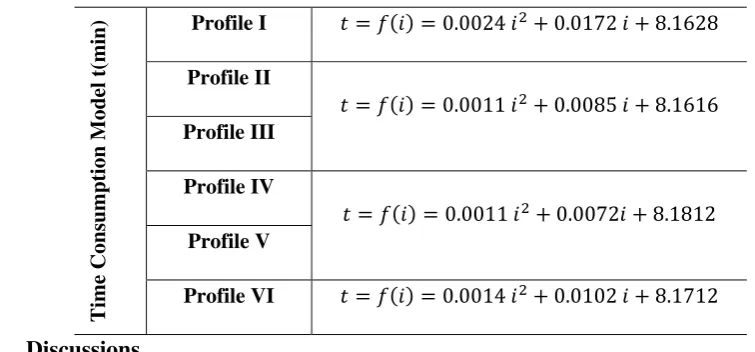
Table 5 shows time consumption model for each standard vertical profile mentioned previously. Based on the implied analysis mentioned earlier, the following results are established:

(1) Time consumption model is a quadratic function for all profiles. The R-square values for all models are more than 99% as shown in the figures 15, 16, 17, and 18.

(2) The results show that the time consumption is similar for the profiles that have symmetrical sketch with a horizontal axis, whereas unsymmetrical sketch of different profiles have different values of time consumption.

(3) Profiles No.2 and No.3 have the same model of time consumption. Correspondingly, Profiles No.4 and No. 5 have the same model, (Table 5).

(4) Time consumption increases with the increasing of maximum gradient value for each profile. (5) The percentage of increasing in time consumption between the first and the last value of

gradient for each profile is 33.6% for profile No.1, 16.3% for profiles No.2 and No.3, 14.9% for profiles No.4 and No.5 and it is 20% for profile No.6.

E = f ( D ) = 0.0257 D3_{- 3.22 D}2_{+ 137.43 D + 2732}

R² = 1

4500 4600 4700 4800 4900 5000

20 30 40 50

_{D (km)}

E (R

Figure 14: Unit force curve of type 3 China Railway High-speed (CRH) Electrical Motor train

Unit (EMU)

Figure 15: Time consumption graph for

profile I

Figure 16: Time consumption graph for

profile II/III

Figure 17: Time consumption graph for

profile IV/V

Figure 18: Time consumption graph for

Table 3: Maximum gradient values for different maximum speed of CH3 – EMU

V (km/h) 350 300 250 200

w0(N/kN) 17.69 13.28 9.52 6.43

imax (‰) 3.96 11.98 20.79 31.46

Table 4: Main technical parameters of five types of CRH-EMU

Locomotive model

Item

CRH 1 CRH 2 CRH 3 CRH 4 CRH 5

Marshalled form 2×[2M+1T]

+[1M+1T]

[4M+4T] /[6M+2T]

2×[2M+1T]

+2T 6M+2T

[3M+1T] +[2M+2T]

Capacity (person) 668 610 610 610 620+2

Group mass (t) 420.4 359.7 380.0 451.0

Group length (m) 213.5 201.4 200.0 201.4 451.0

Operation speed

(Km/h) 200 200/300 350 330 200 Length of front of

motorcar (mm) 26 950 25 700 25 675 25 700 27 600 Length of middle of

motorcar (mm) 26 6000 25 000 24 775 25 000 25 000 Motorcar width (mm) 3 328 3 380 2 950 3 380 3 200

Motorcar height

(mm) 4 040 3 700 3 890 3 700 4 270 Dynamic axle type

Bogie fixed wheel

base (mm) 2 700 2 500 2 500 2 500 2 700 Bogie center distance

(m) 17.500 17.500 17.375 17.500 17.500

Bogie wheel diameter

(mm) 915 ~ 835 860 ~ 790 860 ~ 790

860 ~

790 890 ~ 810

Axle load/readiness

Total traction power

(KW) 5 500

4 800 / 7

200 2 400 5 500

Single motor power

(KW) 275 300 500 300 550

Average power per

ton (KW/t) 13.08 13.34 21.05 19.67 12.19 Starting tractive force

(KN) 325 237 300 300

Starting acceleration

(m/s2) 0.5 0.406 0.406 0.6

Emergency braking

distance (m) ≤ 2 000 ≤ 1800 ≤ 1800 ≤ 2 000

Table 5: Time consumption model for the sixth profiles

Time

C

onsumption Mo

del

t(

mi

n) Profile I 0.0024 0.0172 8.1628

Profile II

0.0011 0.0085 8.1616 Profile III

Profile IV

0.0011 0.0072 8.1812 Profile V

Profile VI 0.0014 0.0102 8.1712

5. Discussions

Based on the normal railway schemes for calculation of time consumption and operating expenses, this study implied the models and graphs, as presented in Figure 2 and Figure 3, for HSR. The study has assessed the effect of stations spacing on operating expenses. In this regard, six standard vertical profiles of HSR line have been studied. The results reported that operating expenses model is a third-degree function of station spacing. These models have applied to a case study. The study shows that when the distance between stations is small like in mountain areas, the operating expenses will be lower. Whereas when the distance between stations is large like in plain areas, the operating expenses will be higher.

consumption will be higher. Meanwhile, when the high-speed train passes through flat or plain areas, there will be less number of intermediate stations.

6. Conclusions and Future Directions

This paper have studied the relationship between operating expenses of HSR line with the station spacing depending on six standard vertical profiles and keeping other indicators constant. We studied the relationship between time consumption and maximum gradient of high-speed railway, but in fact there are few more indicators that can be considered for calculation. Comparison of several times with the vertical sections of existing HSR lines, the intended graphical method shows high degree of veracity among standard profiles. Therefore, future studies can be concentrated on operating expenses, extending time consumption models and including other indicators.

References

 Abid, M., M., Khan, M., B. (2015). Sensitivity analysis of train schedule of a railway track network using an optimization modeling technique. Eur. Transp. Res. Rev. (2015) 7:3.

 Ashiya M., and Yasuda M. (1994). Total system simulation of electrical railway of power consumption study. Paper presented at the 4th International Conference on Computer Aided Design, Manufacture and Operation in the Railway and Other Mass Transit Systems. Part 1 (of 2). Madrid, Spain.

 Aurélie J. (2011), High-speed rail & sustainability. Report for International Union of Railway (UIC), High Speed and Sustainable Development Departments, Paris, France.

 Carrion C., and Levinson D. (2012). Value of travel time reliability: a review of current evidence. Transportation Research Part A: Policy and Practice 46(4), 72-741. DOI: 10.1016/j.tra.2012.01.003  Coto-Millán P., Inglada V., and Casares P. (2011). Social profitability threshold of high-speed

railway: a benefit-cost analysis. Journal of Transportation Technologies 1(4), 107-115, DOI:10.4236/jtts.2011.14014

 Ennio C., and Pierluigi C. (2014). High Speed Rail (HSR) Induced Demand Models. Procedia - Social and Behavioral Sciences 111, 147-156, DOI:10.1016/j.sbspro.2014.01.047

 Gong D.Q. (2010). Design for network of high-speed rail system station spacing. Paper presented at UIC high-speed 2010, the 7th world congress on High Speed Rail. Beijing, China.

 Hang Z. J. (2011). The impact of the high-speed train in China. 2011 International Conference on Management and Service Science, IEEE, Wuhan, China. DOI: 10.1109/ICMSS.2011.5998237  High-Level Group (1995). Relevance of the trans-European high-speed train network for the

European Union: study results. High Speed Europe. Office for Official Publications of the European Communities, 54-55, Luxembourg.

 Hwang H. S. (1998). Control strategy for optimal compromise between trip time and energy consumption in a high-speed railway. Systems, Man and Cybernetics, Part A: IEEE Transactions on Systems and Humans 28(6), DOI: 10.1109/3468.725350

 Levinson D., Mathieu J. M., Gillen D., Kanafani A. (1997). The full cost of high-speed rail: an engineering approach. The Annals of Regional Science, Springer-Verlag 31(2): 189-215, DOI: 10.1007/s001680050045

 Lingaitis, V. (2009). Effectiveness of investments in the development of road infrastructure: Doctoral Thesis Vilnius Gediminas Technical University.

 Qiu D.W., Du M. Y., Lu S. Q., and Shi R. M. (2009). High-speed railway location design using GIS. International Geoscience and Remote Sensing Symposium, IEEE, Cape Town, South Africa. DOI: 10.1109/IGARSS.2009.5418170

 Robert N., and Daniel J. G. (2012). Marginal productivity of expanding highway capacity. Journal of Transport Economics and Policy 46(3), 333–347.

 Vytautas L., and Gintaras S. (2014). Passenger Transport by Railway: Evaluation of Economic and Social Phenomenon. Procedia, Social and Behavioral Sciences 110, 549-559, DOI:10.1016/j.sbspro.2013.12.899

 Wang D., and Wang D.S. (2000). Synthetic optimization in engineering decisions with railway examples. Chengdu, China, Southwest Jiaotong University Press ISBN: 7-81057-391-8.

 Xiang R., Lu G. Y., and He D. (2010). Simulated annealing algorithm for solving a bi-level optimization model on high-speed railway station location. 3rd International Conference on Information and Computing, IEEE. College of traffic and transportation, Southwest Jiaotong University, Chengdu, China.

 Yi S.R. (2008). Railway line selection curriculum design instruction (2nd edi.). Southwest Jiaotong University Press, Chengdu, China.

 Yi S.R., and He H.W. (2009), Railway location design(3rd Ed.). Chengdu, China, Southwest Jiaotong University Press.

 Zeng J., Liu Y. J., and Lin Y. Y. (2013). Pricing model of train passenger transport based on the value of travel time and bi-level programming. International Conference on Management Science and Engineering, IEEE, Harbin, China. DOI: 10.1109/ICMSE.2013.6586311