Forecasting German Car Sales Using Google Data and Multivariate Models

(1)

Munich Personal RePEc Archive

Forecasting German Car Sales Using

Google Data and Multivariate Models

Fantazzini, Dean and Toktamysova, Zhamal

Moscow School of Economics, Moscow State University (Russia),

Faculty of Economics, Higher School of Economics, Moscow (Russia)

2015

Online at

https://mpra.ub.uni-muenchen.de/67110/

(2)

Forecasting German Car Sales Using Google Data and

Multivariate Models

Dean Fantazzini

∗

Zhamal Toktamysova

†

Abstract

Long-term forecasts are of key importance for the car industry due to the lengthy period of time

required for the development and production processes. With this in mind, this paper proposes new

multivariate models to forecast monthly car sales data using economic variables and Google online

search data. An out-of-sample forecasting comparison with forecast horizons up to 2 years ahead

was implemented using the monthly sales of ten car brands in Germany for the period from 2001M1

to 2014M6. Models including Google search data statistically outperformed the competing models

for most of the car brands and forecast horizons. These results also hold after several robustness

checks which consider nonlinear models, different out-of-sample forecasts, directional accuracy, the

variability of Google data and additional car brands.

Keywords

: Car Sales, Forecasting, Google, Google Trends, Global Financial Crisis, Great

Reces-sion.

JEL classification

: C22, C32, C52, C53, L62.

∗

Moscow School of Economics, Moscow State University, Leninskie Gory, 1, Building 61, 119992, Moscow, Russia. Fax:

+7 4955105256 . Phone: +7 4955105267 . E-mail:

[email protected]

.

†

Faculty of Economics, Higher School of Economics, Moscow (Russia)

This is the working paper version of the paper

Forecasting German Car Sales Using Google Data and Multivariate Models

,

(3)

1

Introduction

Long-term forecasting of car sales plays an important role in the automobile industry. Accurate

pre-dictions allow firms to improve market performance, minimize profit losses, and plan manufacturing

processes and marketing policies more efficiently.

Tough competition, significant investments, and the need for quick model updates are the specifics of

the automotive industry which make forecasting an element of key importance for the sales and production

processes. Like other complex industries, it can be characterized by long product development cycles

varying from 12 up to 60 months. An effective planning of the production therefore requires accurate

long-term sales forecasts. Inaccurate forecasts may result in several negative consequences, such as

overstocking or shortage of production supplies, high costs for different workforce activities, loss of

reputation for the manufacturer and even bankruptcy.

There are several economic factors affecting the automobile industry, and they can be broadly

di-vided into three groups. The first group incorporates the technological aspects of the products: quality,

innovation and technology, performance and economy of the engine, functionality, safety, space

man-agement, design and aesthetics (Lin and Zhang, 2004; Sa-ngasoongsong and Bukkapatnam, 2011). The

second group comprises promotion and sales factors, including wholesale and retail prices, customer

ser-vice, advertising campaigns, and brand image (Landwehr, Labroo, and Herrmann, 2011). These factors

are significant, but usually do not have a long-term effect and automobile producers in most cases can

manage and control them (Dekimpe, Hanssens, and Silva-Risso, 1998; Nijs, Dekimpe, Steenkamp, and

Hanssens, 2001; Pauwels, Hanssens, and Siddarth, 2002; Pauwels, Silva-Risso, Srinivasan, and Hanssens,

2004). The third group includes various political, economic and social environmental factors which are

generally beyond the control of manufacturers, such as organizational issues, political issues, global

eco-nomic growth, ecological and physical forces, socio-cultural effects and consumer behavior. The use of

these factors for car sales forecasting has been rather limited, see Br¨

uhl, Borscheid, Friedrich, and

Re-ith (2009), Shahabuddin (2009), Wang, Chang, and Tzeng (2011) and Sa-ngasoongsong, Bukkapatnam,

Kim, Iyer, and Suresh (2012). Moreover, most previous studies have focused on the dynamics of car

sales in the short-term, with forecast horizons usually less than 4 months, whereas car sales forecasting

requires time scales with duration up to one year or more.

Following the growing number of Internet users (International Telecommunications Union, 2014)

and the increasing popularity of Google as a search engine for obtaining information about cars, we

propose the use of Google search data as a leading indicator for the long-term forecasting of car sales.

In this regard, Google Search holds the world leadership among all search engines with a 54% market

share (Net Applications, 2014). Since 2004, it has offered a tool called Google Trends, which provides

information on the relative interest of users in a particular search query, at a given geographic region and

at a given time (the data are available on a weekly or even daily basis). Moreover, Google Trends can

attribute queries to different search categories (Autos, Computers, Finance, Health and others). In recent

years, researchers worldwide have begun to use online search data to produce real-time forecasts where

information from official sources is released with a lag (such as ‘nowcasting’), or simply as an additional

variable for forecasting purposes, see Choi and Varian (2012), Askitas and Zimmermann (2009), Suhoy

(2009), Ginsberg, Mohebbi, Patel, Brammer, Smolinski, and Brilliant (2009), Da, Engelberg, and Pengjie

(2011), D’Amuri and Marcucci (2013) and Fantazzini and Fomichev (2014) for some recent applications.

With this in mind, we propose a set of models for the long-term forecasting of car sales in Germany,

which consider both economic variables and online search queries. Germany is the third biggest car

producer in the world (about 14 million vehicles in 2013 and 20% of the total world production) and

the absolute leader in Europe (31% of the total European production), see the reports by the German

Association of the Automotive Industry (GTAI, 2014) and the Germany Trade and Invest Organization

(VDA, 2014) for more details. As for Internet users, Germany has the second highest number of users

in Europe (12.3% of all European users) and the 7th in the world. In June 2014, more than 71 million

people in Germany visited the Web at least once a month, representing 88.6% of the adult population

(Internet World Stats, 2014).

(4)

multivariate models for both deseasonalized data, the usual approach in the economic literature, and

for data not seasonally adjusted, which is more common in practice, since planning and production

departments tend to work with raw data

1

.

The second contribution of our paper is a large-scale forecasting exercise for ten car brands in

Ger-many, where we compute out-of-sample forecasts ranging from 1 month to 24 months ahead. Our results

show that models including car sales, Google data and economic variables outperform the competing

models in the medium term for most of the car brands, while multivariate models including only car

sales and Google data outperform the other models for long-term forecasts up to 24 steps ahead. The use

of parsimonious models is crucial to obtain precise forecasts in the long run, and the use of Google search

data represents a simple and powerful way to summarize the large amount of information available (see

also Fantazzini and Fomichev, 2014).

The third contribution of the paper is a set of robustness checks to verify that our results also hold

when considering nonlinear models, different out-of-sample forecasts, the use of directional accuracy as

the main evaluation tool, Google data downloaded on different days, and additional car brands.

The paper is organized as follows. Section 2 describes the data and the in-sample analysis, and the

forecasting models and their out-of-sample performance are reported in Section 3. Robustness checks

are discussed in Section 4, and Section 5 briefly concludes.

2

Data and In-Sample analysis

We analyze new car registrations in the Federal Republic of Germany, as provided in press releases

by the Federal Motor Transport Authority (Kraftfahrt-Bundesamt). These data cover the period from

January 2001 to June 2014, for a total of 162 observations. The data consist of monthly numbers of

new vehicle registrations by vehicle type and new registrations of passenger cars by brand starting from

2001. For different reasons, the information for some car brands was truncated: certain brands were

present only after 2001; others stopped being observed well before 2014; or the registration statistics

were not published due to the small number of registrations per month. Our car brands were selected

based on the availability of a long time series for new car registrations and their presence in the “

Vehicle

Brands

” Google subcategory. Moreover, car brands were chosen to reflect both foreign and domestic car

producers.

There were only 22 brands which had both monthly data continuously available since 2001 and were

present in Google Trends. We divided these brands into clusters by taking the average sales for each

brand and using the method of k-means with Euclidian distance. We wanted to determine large, medium

and small car manufacturers, and assign all brands into three clusters. The method of k-means allowed us

to define the number of clusters a priori and minimize the within-cluster distance while maximizing the

between-cluster distance (see e.g. Hartigan (1975)). The initial

k

cluster centers are chosen to maximize

the initial distance. The data are arranged to the nearest cluster center, therefore

k

clusters are formed.

Next, new cluster centers are chosen as centers of mass for the clusters. After recalculation, the data are

again assigned to the nearest cluster centers. The procedure ends when all centers of mass are stabilized.

We found three clusters consisting of the following brands:

•

Large sellers: Volkswagen, Opel, Ford, BMW, Audi (average monthly sales between 19523 and

53820);

•

Medium-sized sellers: Renault, Toyota, Peugeot, Hyundai, Fiat, Mazda, Citroen, Nissan (average

monthly sales between 4976 and 14074);

•

Small sellers: Jaguar, Kia, Land Rover, Porsche, Subaru, Honda, Volvo, Mitsubishi, Suzuki (average

monthly sales between 355 and 3351).

We also used the method of k-means with the monthly sales data from January 2001 to June 2014 and

we obtained the same division into three clusters.

For the sake of space, interest and to keep the empirical analysis computationally tractable,

through-out the paper we will consider three large sellers (Volkswagen, Opel, BMW), three medium-sized sellers

(Toyota, Fiat, Citroen), and four small sellers (Jaguar, Kia, Mitsubishi, Suzuki). The remaining 12

brands will be examined as a robustness check in section 4.5.

(5)

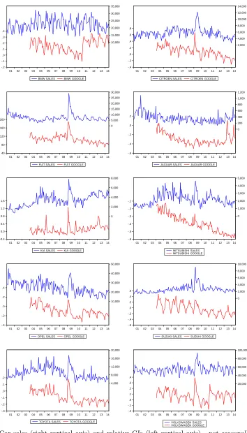
The plots of the monthly sales are reported in Figure 1 (right vertical axis). Car sales are subject to

seasonal fluctuations and all car brands tend to show several peaks during the year, with the biggest one

taking place at the end of spring. In general, car sales decline during winter. The Census X-12 tests for

seasonality detected that all brands exhibit stable seasonality, with no evidence of moving seasonality.

The second source of data consists of Google Trends data, which can be downloaded from

www.google.

com/trends/

, using the specific “

Autos and Vehicles

” category and its “

Vehicle Brands

”

subcate-gory. The Google Index (GI) is the ratio of the number of queries relative to a particular category (in

our case the car brand), with respect to all queries in the selected region at a given point of time. The

data were collected for the whole of Germany for the period January 2004 - June 2014. The data have a

weekly frequency and were converted to a monthly series by taking average values. While the GIs for a

keyword are normalized to be bounded between 0 to 100, where 100 is the peak of the search queries, the

GIs for a category are expressed in terms of percentage change from their first observation in January

2004, so that they can be both positive and negative. Their plots are reported in Figure 1 (left vertical

axis): it is interesting to note that the turning points in the GIs anticipate those in the car sales for

all car brands. This initial evidence suggests that Google data may be of some help for medium- and

long-term forecasting.

Additionally, we included a number of economic variables related to car sales, based on recent works

by Shahabuddin (2009) and Sa-ngasoongsong, Bukkapatnam, Kim, Iyer, and Suresh (2012). These

variables are assumed to reflect the state of the national economy, and the factors that can influence

a consumer’s decision to purchase a car. The selected economic variables and their descriptions are

presented in Table 1. The data were collected for the period January 2001 to June 2014. All data,

with the exception of building construction orders (which were available only seasonally adjusted), show

some form of seasonality, with peaks during the summer season and troughs at the end of the year. The

quarterly GDP data were converted to monthly data via the quadratic match average procedure, while

the daily data for Euribor rates were transformed into monthly data by taking their average. Their plots

are reported in Figure 2.

Economic variable

Frequency

Seasonally

adjusted

Source

Explanation

Building

Construction

(BC)

M

yes

GFB

Volume index of new orders for residential

buildings construction

Consumer Confidence

Indi-cator (CCI)

M

no

DG ECFIN

Consumer survey that reflects consumer

ex-pectations

Consumer

Price

Index

(CPI)

M

no

FSO

Measure of the ratio of a price of fixed set of

consumer goods and services in current period

to its price in a basic period

Euro

Interbank

Offered

Rate (EURIBOR)

D

no

EBF

Calculated as an average rate of lending rate of

the banks which participate in the survey. For

the current research EURIBOR for long-term

credits (1 year) is considered

Gross Domestic Product

(GDP)

Q

no

FSO

Market value of all goods and services

pro-duced within a country. In the present work

GDP in nominal billions Euro was taken

Production Index (PI)

M

no

FSO

Production Index for durable goods

Unemployment Rate (UR)

M

no

FEA

The registered unemployed population as a

percentage of the civilian labor force

Petrol Price (PP)

M

no

FSO

Consumer price for petrol, price index

Table 1: Description of economic variables used in the analysis. The second column reports the frequency

of publishing: M - monthly data, Q - quarterly data, D - daily data. The abbreviations used in the

fourth column represent the data sources: GFB - German Federal Bank (Deutsche Bundesbank), DG

ECFIN -Directorate General for Economic and Financial Affairs, FSO - The Federal Statistical Office

(Statistisches Bundesamt), EBF - The European Banking Federation, FEA - The Federal Employment

Agency (Bundesagentur f¨

ur Arbeit).

Data with seasonal behavior were seasonally adjusted with the Census X-12 adjustment program

developed by US Census Bureau. However, we also considered the raw data, since they are more common

in practice and of greater interest for production planners and marketing managers, who base their

decisions on real data which exhibit seasonality.

(6)

-.2 -.1 .0 .1 .2 .3 .4 10,000 15,000 20,000 25,000 30,000 35,000

01 02 03 04 05 06 07 08 09 10 11 12 13 14

BMW SALES BMW GOOGLE

-.4 -.2 .0 .2 .4 .6 .8 2,000 4,000 6,000 8,000 10,000 12,000 14,000

01 02 03 04 05 06 07 08 09 10 11 12 13 14

CITROEN SALES CITROEN GOOGLE

40 80 120 160 200 0 5,000 10,000 15,000 20,000 25,000 30,000

01 02 03 04 05 06 07 08 09 10 11 12 13 14

FIAT SALES FIAT GOOGLE

-.6 -.4 -.2 .0 .2 0 200 400 600 800 1,000 1,200

01 02 03 04 05 06 07 08 09 10 11 12 13 14

JAGUAR SALES JAGUAR GOOGLE

-0.4 0.0 0.4 0.8 1.2 1.6 0 2,000 4,000 6,000 8,000

01 02 03 04 05 06 07 08 09 10 11 12 13 14

KIA SALES KIA GOOGLE

-.6 -.5 -.4 -.3 -.2 -.1 0 1,000 2,000 3,000 4,000 5,000

01 02 03 04 05 06 07 08 09 10 11 12 13 14

MITSUBISHI SALES MITSUBISHI GOOGLE

-.4 -.2 .0 .2 .4 10,000 20,000 30,000 40,000 50,000

01 02 03 04 05 06 07 08 09 10 11 12 13 14

OPEL SALES OPEL GOOGLE

-.6 -.4 -.2 .0 .2 .4 .6 0 2,000 4,000 6,000 8,000 10,000

01 02 03 04 05 06 07 08 09 10 11 12 13 14

SUZUKI SALES SUZUKI GOOGLE

-.3 -.2 -.1 .0 .1 .2 4,000 8,000 12,000 16,000 20,000

01 02 03 04 05 06 07 08 09 10 11 12 13 14

TOYOTA SALES TOYOTA GOOGLE

-.2 -.1 .0 .1 .2 .3 .4 20,000 40,000 60,000 80,000 100,000

01 02 03 04 05 06 07 08 09 10 11 12 13 14

[image:6.612.119.473.48.668.2]

VOLKSWAGEN SALES VOLKSWAGEN GOOGLE

(7)

60 80 100 120 140 160 180 200

010203 040506 07080910 111213 14

BUILDING CONSTRUCTION ORDERS

60 70 80 90 100 110 120

01020304 050607 08091011 1213 14

CONSUMER CONFIDENCE INDEX

85 90 95 100 105 110

01 02030405 060708 09101112 13 14

CPI 0 1 2 3 4 5 6

0102 03040506 070809 101112 13 14

EURIBOR 500 550 600 650 700 750

010203 040506 07080910 111213 14

GDP 70 80 90 100 110 120 130 140

01020304 050607 08091011 1213 14

PRODUCTION INDEX 6 7 8 9 10 11 12 13

01 02030405 060708 09101112 13 14

UNEMPLOYMENT RATE

70 80 90 100 110 120 130 140

0102 03040506 070809 101112 13 14

PETROL PRICE

Figure 2: Economic variables - not seasonally adjusted. Sample: 2001M1 - 2014M6

linear patterns

2

(see Sa-ngasoongsong, Bukkapatnam, Kim, Iyer, and Suresh (2012)). The descriptive

statistics for the car registrations, the Google data and the economic variables (both seasonally adjusted

and raw data) are not reported for the sake of space and are available from the authors upon request.

To select the best multivariate model for each car brand, we follow the structural relationship

identi-fication methodology discussed by Sa-ngasoongsong, Bukkapatnam, Kim, Iyer, and Suresh (2012) for the

case of the US car market. Briefly, the first step is to identify the order of integration using unit root tests;

if all variables are stationary, VAR and VARX (Vector Autoregressive with exogenous variables) models

are used. The second step determines the exogeneity of each variable using the sequential reduction

method for weak exogeneity by Hall, Henry, and Greenslade (2002), who consider weakly exogenous each

variable for which the test is not rejected and re-test the remaining variables until all weakly exogenous

variables are identified. For non-stationary variables, cointegration rank tests are employed to determine

the presence of a long-run relationship among the endogenous variables: if this is the case, VECM or

VECMX (Vector Error Correction model with exogenous variables) models are used, otherwise VAR or

VARX models in differences are applied. The last step is to compute the impulse response functions

from the chosen model to trace the effect of a unit shock in one of the variables on the future values

of car sales, and to compute out-of-sample forecasts (see Sa-ngasoongsong, Bukkapatnam, Kim, Iyer,

and Suresh (2012) for more details). Our approach differs from the one proposed by Sa-ngasoongsong,

Bukkapatnam, Kim, Iyer, and Suresh (2012) in two respects: first, we employ unit root tests and

coin-tegration tests allowing for structural breaks, given the possible break in the years 2008-2009 during the

global financial crisis. Second, we employ the previous identification methodology for both the seasonally

adjusted data and the raw data.

2.1

Stationarity

2.1.1

Seasonally Adjusted data

The stationarity of our variables is analyzed using several unit root tests allowing for potential endogenous

structural break(s), both under the null of a unit root and under the alternative. We justify this choice

considering the strong influence the global financial crisis in the years 2007-2009 had on the German

economy, which is visible when looking at Figures 1 and 2. As for the Google data, we remark that the

statistical effects of dividing the original search data by the total number of web searches in the same

week and area are unknown, so that we cannot say a priori whether they are stationary or not (see also

Fantazzini and Fomichev (2014) for a discussion on this issue). More specifically, we employed four unit

root tests: the Lee and Strazicich (2003) unit root tests allowing for one and two breaks, respectively, and

the Range Unit Root (RUR) and the Forward-Backward RUR tests suggested by Aparicio, Escribano,

and Garcia (2006), which are non-parametric tests robust against nonlinearities, error distributions,

structural breaks and outliers. A brief description of these tests is reported in the Technical Appendix

(8)

A accompanying this paper and can be found on the authors’ websites.

RUR

FB

LS 1 break

LS 2 breaks

The null hypothesis

Test

is rejected

statistic

by all tests?

Car sales

BMW

0.71 *

1.16

-5.08

*

-11.14

*

no

Citroen

1.34

1.95

-5.12

*

-6.09

*

no

Fiat

0.79 *

1.89

-4.75

*

-6.31

*

no

Jaguar

0.87 *

1.39

-4.47

-6.98

*

no

Kia

1.42

2.01

-4.94

*

-5.89

*

no

Mitsubishi

0.79 *

1.34

-5.05

*

-5.79

*

no

Opel

0.87 *

1.56

-6.17

*

-6.87

*

no

Suzuki

1.02 *

1.67

-4.91

*

-6.47

*

no

Toyota

1.50

1.95

-4.92

*

-5.86

*

no

Volkswagen

0.87 *

1.73

-6.66

*

-7.52

*

no

Economic variables

BUILD

1.34

2.17

-2.33

-8.68

*

no

CCI

1.18

2.23

-3.60

-4.07

no

CPI

9.14 *

13.15*

-3.53

-4.10

no

EURIBOR

3.07

3.73 *

-3.46

-4.29

no

PP

2.68

3.96 *

-3.65

-5.26

no

GDP

6.30 *

8.75 *

-3.67

-4.53

no

PI

1.42

1.67

-3.88

-4.80

no

UR

5.28 *

7.30 *

-3.42

-5.66

no

Google data

BMW GI

1.34

1.77

-5.24

*

-8.59

*

no

Citroen GI

1.97

2.34

-5.98

*

-6.71

*

no

Fiat GI

1.43

2.34

-4.59

*

-7.07

*

no

Jaguar GI

1.52

1.90

-7.12

*

-8.10

*

no

Kia GI

0.80 *

1.39

-7.45

*

-8.12

*

no

Mitsubishi GI

2.68

2.97

-9.26

*

-9.83

*

no

Opel GI

1.25

2.53

-4.51

*

-5.24

no

Suzuki GI

1.88

2.09

-7.18

*

-8.24

*

no

Toyota GI

1.34

1.90

-4.67

*

-5.17

no

[image:8.612.122.475.61.340.2]

Volkswagen GI

1.34

1.83

-4.96

*

-5.55

no

Table 2: Unit root tests: RUR = Range Unit Root test by Aparicio, Escribano, and Garcia (2006); FB

= Forward-Backward RUR test by Aparicio, Escribano, and Garcia (2006); LS = Unit Root test by Lee

and Strazicich (2003). Null hypothesis: the time series has a unit root.

* Significance at the 5% level.

The results in Table 2 show that the majority of our time series are not stationary. However, the

Lee and Strazicich (2003) tests show a stronger evidence of unit roots for economic variables, while the

Aparicio, Escribano, and Garcia (2006) tests show the same for car sales and Google data. If we follow

a conservative approach and analyze when all four tests reject the null hypothesis (see the last column

in Table 2), then all car brands can be deemed non-stationary.

2.1.2

Raw data

To test the null hypothesis of a periodic unit root, we follow the two-step strategy suggested by Boswijk

and Franses (1996) and Franses and Paap (2004). In the first step, a likelihood ratio test for testing a

single unit root in a Periodic Auto-Regressive (PAR) model of order

p

is performed. Since there is no

version of this test with endogenous breaks, we estimated it both with the full sample starting in 2001,

and with a smaller sample starting in 2008. The year 2008 was chosen following the previous evidence

of a possible break in this year, which emerged with the unit root tests allowing for breaks in the case

of seasonally adjusted data. If the null of a periodic unit root cannot be rejected, Boswijk and Franses

(1996) and Franses and Paap (2004) suggest to test in a second step whether the process contains a

non-periodic unit root equal to 1 for all seasons. A description of these tests is reported in the Technical

Appendix B.

(9)

Sample: 2001-2014

Sample: 2008-2014

1st step

2nd step

1st step

2nd step

H

0

: periodic

H

0

: non periodic

H

0

: periodic

H

0

: non periodic

unit root

Car Sales

BMW

NC

Citroen

18.66*

/

7.21

0.46

Fiat

16.60*

/

4.43

0.00

Jaguar

42.41*

/

NC

Kia

10.46*

/

4.96

0.08

Mitsubishi

22.97*

/

16.96*

/

Opel

15.38*

/

10.66*

/

Suzuki

24.85*

/

15.95*

/

Toyota

10.19*

/

15.81*

/

Volkswagen

58.20*

/

NC

Economic Variables

BUILD

7.99

0.09

2.32

0.11

CCI

3.23

0.06

1.02

0.14

CPI

0.13

0.00

0.30

0.44

EURIBOR

0.37

0.66

1.99

0.15

PP

1.97

0.88

1.36

0.10

GDP

0.01

0.00

0.15

0.00

PI

36.79*

/

22.07*

/

UR

0.52

0.56

NC

Google data

BMW GI

8.93

0.49

2.71

0.53

Citroen GI

4.90

0.47

4.46

0.13

Fiat GI

4.47

0.04

1.84

0.11

Jaguar GI

12.02*

/

5.17

0.01

Kia GI

16.82*

/

8.07

0.76

Mitsubishi GI

3.91

0.99

2.19

0.35

Opel GI

6.06

0.64

6.69

0.53

Suzuki GI

3.60

0.02

3.63

0.04

Toyota GI

5.86

0.46

5.15

0.01

[image:9.612.124.472.39.320.2]

Volkswagen GI

11.20*

/

5.38

0.39

Table 3: Periodic Unit root tests by Boswijk and Franses (1996) and Franses and Paap (2004).

* Significance at the 5% level. NC = Not Converged. The second step is performed only if the first step

numerically converged and did not reject the null hypothesis.

p-values smaller than 0.05 are in bold.

2.2

Weak Exogeneity and Cointegration Tests

2.2.1

The next step in the structural relationship identification methodology discussed by Sa-ngasoongsong,

Bukkapatnam, Kim, Iyer, and Suresh (2012) is to determine the exogeneity of each variable using the

sequential reduction method for weak exogeneity proposed by Hall, Henry, and Greenslade (2002). This

method exogenizes all weakly exogenous variables and re-tests the remaining variables until all weakly

exogenous variables are identified. The variables that reject the null of weak exogeneity after re-testing

are reported in Table 12 in Appendix A: the Euribor series can be considered weakly exogenous for four

car brands, while almost all other variables are deemed endogenous (with some exceptions for Mitsubishi).

We then proceeded to test for cointegration using the variables which were deemed endogenous

according to the previous sequential test procedure by Hall, Henry, and Greenslade (2002). We test for

cointegration using a set of cointegration tests allowing for the presence of structural break(s):

•

Gregory and Hansen (1996) single-equation cointegration test allowing for one endogenous break;

•

Hatemi (2008) single-equation cointegration test allowing for two endogenous breaks;

•

Johansen, Mosconi, and Nielsen (2000) multivariate test allowing for the presence of one or two

exogenous break(s), where the dates of the breaks are the ones selected by the Gregory and Hansen

(1996) and Hatemi (2008) tests, respectively.

(10)

and Nielsen (2000) is that they allow only for exogenous breaks. Accordingly, we followed a 2-step

strategy: we first estimated the single-equation tests to obtain an indication of the structural break dates.

We then used these dates to compute the tests by Johansen, Mosconi, and Nielsen (2000). Finally, we

remark that the number of lags for the Johansen tests were chosen to minimize the Schwartz criterion

and to make the residuals approximately white noise.

Single-Equation cointegration tests

Gregory and Hansen (1996)

Hatemi (2008)

one(endogenous) break

two(endogenous) breaks

Z-t statistic

Break date

Z-t statistic

Break dates

BMW

-10.61*

2010M02

-11.14*

2006M09 2008M07

Citroen

-7.38*

2009M02

-8.35

2005M08 2007M07

Fiat

-7.54*

2006M01

-8.27

2005M11 2007M08

Jaguar

-14.54*

2012M09

-14.30*

2007M10 2011M02

Kia

-8.27*

2006M09

-8.61

2006M09 2011M01

Mitsubishi

-10.98*

2009M03

-10.79*

2008M04 2008M12

Opel

-8.72*

2009M02

-7.60

2009M09 2010M10

Suzuki

-10.85*

2009M02

-10.14

2006M09 2007M06

Toyota

-7.95*

2009M12

-8.40

2006M09 2009M07

Volkswagen

-9.96*

2009M03

-9.35

2005M08 2007M08

Multivariate cointegration tests

Johansen (1995)

Johansen, Mosconi, and Nielsen (2000)

No Breaks

one(exogenous) break

two (exogenous) breaks

N. of CEs

Break date

N. of CEs

Break dates

at 5% level

(GH,1996)

at 5% level

(H,2008)

BMW

5 CE

2010M02

5 CE

2006M09 2008M07

Citroen

5 CE

4 CE

2009M02

5 CE

2005M08 2007M07

Fiat

7 CE

5 CE

2006M01

7 CE

2005M11 2007M08

Jaguar

5 CE

4 CE

2012M09

5 CE

2007M10 2011M02

Kia

5 CE

3 CE

2006M09

4 CE

2006M09 2011M01

Mitsubishi

4 CE

0 CE

2009M03

NC

2008M04 2008M12

Opel

5 CE

4 CE

2009M02

5 CE

2009M09 2010M10

Suzuki

5 CE

2009M02

NC

2006M09 2007M06

Toyota

5 CE

2009M12

5 CE

2006M09 2009M07

[image:10.612.72.543.108.355.2]

Volkswagen

5 CE

2009M03

5 CE

2005M08 2007M08

Table 4: Single-equation and multivariate cointegration tests with and without structural break(s) for

seasonally-adjusted data. The null hypothesis for all tests is the absence of cointegration. The tests

considered the case of a level shift. The table cells for the Johansen tests report the number of CEs

selected at the 5% level. NC=not converged. * Significance at the 5% level.

Table 4 shows that there is strong evidence for cointegration for all considered car brands. However,

structural breaks seem to have a non-negligible effect, particularly when considering Johansen

multi-variate tests. Moreover, the effects of breaks appear to be much stronger for foreign brands than for

domestic brands (BMW, Volkswagen and, to a lesser extent, Opel), for which the cointegration tests do

not change substantially when breaks are taken into account.

2.2.2

Raw data

To determine the exogeneity of variables with potential seasonal behavior, we extend the previous

se-quential reduction method for weak exogeneity by including centered seasonal dummies: they sum to

zero over time and therefore do not affect the asymptotic distributions of the tests (see Johansen (1995,

2006)). The variables that reject the null of weak exogeneity after re-testing are reported in Table 13 in

Appendix A: the results for raw data are not too dissimilar to the seasonally-adjusted data, even though

there are less variables which are weakly exogenous. We then tested for cointegration using the

vari-ables which were found to be endogenous, and the previous cointegration tests augmented with centered

seasonal dummies, see Table 5.

In the case of raw data, the evidence for cointegration appears to be quite similar to that of

seasonally-adjusted data, particularly when considering the Johansen test without breaks and with one break.

Moreover, the fact that the Johansen test with two breaks failed to converge for some car brands indicates

that our sample is too small for two breaks and that only tests with one break should be considered.

(11)

Single-Equation cointegration tests

Gregory and Hansen (1996)

Hatemi (2008)

one (endogenous) break

two (endogenous) breaks

Z-t statistic

Break date

Z-t statistic

Break dates

BMW

-10.78*

2010M02

11.35*

2006M09 2008M07

Citroen

-7.70*

2009M02

8.60

2005M08 2007M07

Fiat

-7.63*

2005M10

8.64

2005M10 2007M08

Jaguar

-13.10*

2006M11

NC

Kia

-8.71*

2006M09

9.25

2009M09 2011M01

Mitsubishi

-11.54*

2009M02

10.88*

2008M03 2008M12

Opel

-8.48*

2009M02

7.30

2009M09 2010M12

Suzuki

-11.00*

2009M02

9.64

2006M09 2007M07

Toyota

-7.44*

2009M12

8.03

2009M10 2010M12

Volkswagen

-10.67*

2009M02

9.63

2005M08 2007M07

Multivariate cointegration tests

Johansen (1995)

Johansen, Mosconi, and Nielsen (2000)

No Breaks

one(exogenous) break

two(exogenous) breaks

N. of CEs at 5% level

N. of CEs

Break date

N. of CEs

Break dates

at 5% level

(GH,1996)

at 5% level

(H,2008)

BMW

5 CE

4 CE

2010M02

5 CE

2006M09 2008M07

Citroen

5 CE

2009M02

5 CE

2005M08 2007M07

Fiat

5 CE

6 CE

2005M10

7 CE

2005M10 2007M08

Jaguar

3 CE

0 CE

2006M11

NC

Kia

5 CE

2006M09

5 CE

2009M09 2011M01

Mitsubishi

4 CE

2009M02

NC

Opel

5 CE

4 CE

2009M02

5 CE

2009M09 2010M12

Suzuki

5 CE

6 CE

2009M02

NC

Toyota

5 CE

2009M12

5 CE

2009M10 2010M12

[image:11.612.75.547.45.278.2]

Volkswagen

5 CE

6 CE

2009M02

6 CE

2005M08 2007M07

Table 5: Single-equation and multivariate cointegration tests with and without structural break(s) for

raw data. The null hypothesis for all tests is the absence of cointegration. The tests considered the case

of a level shift. The table cells for the Johansen tests report the number of CEs selected at the 5% level.

NC=not converged. * Significance at the 5% level.

parsimonious model can nevertheless be of interest for forecasting purposes. Moreover, the capacity

of Google data to summarize a wealth of information should not be underestimated. In this regard,

we implemented the single-equation periodic cointegration test discussed in Franses and Paap (2004),

which is an extension of the Boswijk (1994) cointegration test. The null hypothesis is the absence of

cointegration against the alternative of periodic cointegration and the right-hand variables should be

weakly exogenous. A description of this test as well as the test for weak exogeneity in the case of

periodic variables by Boswijk (1994) is reported in the Technical Appendix D. Since we are not aware of

any extension of this test allowing for structural breaks, we estimated it using both the full sample and a

reduced sample starting in 2008 to take any potential break into account and the results are reported in

Table 14 in Appendix A: the evidence in favor of periodic cointegration is fairly strong, but the results

of the Boskwijk test statistics change partially when the smaller sample starting in 2008 is considered.

Caution should therefore be exercised when dealing with this restricted model. Interestingly, the GIs are

weakly exogenous with respect to car sales for almost all brands at the 5% level and this outcome does

not change substantially with the sample used.

2.3

Impulse Response Functions

(12)

details about these tests). The full results are available from the authors upon request.

-.04 -.02 .00 .02 .04

1 2 3 4 5 6 7 8 9 10 11 12

Response of LOG(CAR BMW SALES) to LOG(BMW GI)

-.04 -.02 .00 .02 .04

1 2 3 4 5 6 7 8 9 10 11 12

Response of LOG(CAR CITROEN SALES) to LOG(CITROEN GI)

-.04 -.02 .00 .02 .04

1 2 3 4 5 6 7 8 9 10 11 12

Response of LOG(CAR FIAT SALES) to LOG(FIAT GI)

-.04 -.02 .00 .02 .04

1 2 3 4 5 6 7 8 9 10 11 12

Response of LOG(CAR JAGUAR SALES) to LOG(JAGUAR GI)

-.04 -.02 .00 .02 .04

1 2 3 4 5 6 7 8 9 10 11 12

Response of LOG(CAR KIA SALES) to LOG(KIA GI)

-.04 -.02 .00 .02 .04 .06 .08

1 2 3 4 5 6 7 8 9 10 11 12

Response of LOG(CAR MITSUBISHI SALES) to LOG(MITSUBISHI GI)

-.04 -.02 .00 .02 .04

1 2 3 4 5 6 7 8 9 10 11 12

Response of LOG(CAR OPEL SALES) to LOG(OPEL GI)

-.04 -.02 .00 .02 .04

1 2 3 4 5 6 7 8 9 10 11 12

Response of LOG(CAR SUZUKI SALES) to LOG(SUZUKI GI)

-.04 -.02 .00 .02 .04

1 2 3 4 5 6 7 8 9 10 11 12

Response of LOG(CAR TOYOTA SALES) to LOG(TOYOTA GI)

-.04 -.02 .00 .02 .04

1 2 3 4 5 6 7 8 9 10 11 12

[image:12.612.84.511.68.289.2]

Response of LOG(CAR VOLKSWAGEN SALES) to LOG(VOLKSWAGEN GI)

Figure 3: Impulse response functions: response of car sales (in logs) to generalized one standard deviation

innovations in the Google Indexes.

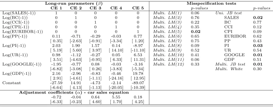
Long-run parameters (

β

)

Misspecification tests

CE 1

CE 2

CE 3

CE 4

CE 5

p

-values

p

-values

Log(SALES(-1))

1

0

Multi. LM(1)

0.06

Uni. JB test

Log(BC(-1))

0

1

0

Multi. LM(2)

0.76

SALES

0.02

Log(CCI(-1))

0

1

0

Multi. LM(3)

0.22

BC

0.77

Log(CPI(-1))

0

1

0

Multi. LM(4)

0.35

CCI

0.12

Log(EURIBOR(-1))

0

1

Multi. LM(5)

0.02

CPI

0.09

[image:12.612.74.539.353.536.2]

Log(PP(-1))

0.11

-0.71

-0.29

-0.03

0.77

Multi. LM(6)

0.65

EURIBOR

0.62

[ 0.35]

[-2.63]

[-0.91]

[-3.34]

[ 1.20]

Multi. LM(7)

0.75

PP

0.43

Log(PI(-1))

2.03

1.90

1.57

0.14

-8.97

Multi. LM(8)

0.09

PI

0.03

[ 5.19]

[ 5.60]

[ 3.97]

[ 14.10]

[-11.10]

Multi. LM(9)

0.52

UR

0.54

Log(UR(-1))

0.98

-1.12

-0.27

0.05

6.53

Multi. LM(10)

0.41

GOOGLE

0.01

[ 3.51]

[-4.63]

[-0.95]

[ 6.33]

[ 11.31]

Multi. LM(11)

0.06

GDP

0.51

Log(GOOGLE(-1))

-1.95

-0.77

0.08

-0.03

-3.16

Multi. LM(12)

0.33

Multi. JB test

0.01

[-6.82]

[-3.08]

[ 0.26]

[-3.83]

[-5.34]

Multi. White

0.30

Log(GDP(-1))

2.16

-2.96

-0.83

-0.46

19.78

[ 2.91]

[-4.61]

[-1.11]

[-24.16]

[ 12.95]

Constant

-27.59

14.91

-4.73

-2.14

-89.07

[-6.64]

[ 4.13]

[-1.13]

[-20.05]

[-10.39]

Adjustment coefficients (

α

) - car sales equation

-0.72

-0.04

0.64

5.55

0.18

[-6.33]

[-0.23]

[ 4.60]

[ 1.70]

[ 4.25]

Table 6: Long-run parameters and adjustment coefficients for the Volkswagen car sales equation (left

table). Misspecification tests on the residuals from the Volkswagen VECMX model (right table).

t-statistics are reported in brackets, while

p-values smaller than 5% are reported in bold.

As expected, a unit shock in the Google Index has a rather long and positive effect for almost all

car brands. Similarly, the model estimates in Table 6 show that the Google Index enters almost all

cointegration equations with significant positive coefficients

3

, while the residual tests do not signal any

serious misspecification.

(13)

3

Out-of-Sample Forecasting Analysis

The last step in the structural relationship identification methodology discussed by Sa-ngasoongsong,

Bukkapatnam, Kim, Iyer, and Suresh (2012) is to compare the forecasting performances of the selected

VECM (or VECMX) models with a set of competitors.

3.1

We compared a set of 34 models, which allow for different degrees of model flexibility, parsimonious

specifications and numerical tractability. More specifically, three types of multivariate models were

employed:

•

Vector Error Correction (VEC) models:

We considered both VECM and VECMX models, as well

as models with and without Google data, to better examine their effects on forecasting performance.

The number of lags was selected to minimize the Schwartz criteria and to make the residuals

ap-proximately white noise. We also considered a set of parsimonious bivariate specifications including

only car sales and Google data, which may be of interest for long-term forecasting.

•

Vector Auto-Regressive (VAR) models:

We considered VAR models with variables in log-levels and

in log-differences, to consider both cases of stationarity and non-stationarity. Moreover, models

with and without exogenous variables and with and without Google data were also considered.

Finally, a set of parsimonious bivariate VAR models including only car sales and Google data was

included.

•

Bayesian Vector Auto-Regressive (BVAR) models:

When there are a lot of variables and a high

number of lags, estimating the parameters of a VAR model can be very difficult, if not impossible.

One way to solve this issue is to shrink the parameters using Bayesian methods. Bayesian VAR

models have recently enjoyed a lot of success in macroeconomic forecasting (see Koop and Korobilis

(2010) for a recent review and Fantazzini and Fomichev (2014) for a recent application with Google

data). In this regard, we used the so-called Litterman/Minnesota prior, which was developed by

researchers at the University of Minnesota and at the Federal Reserve Bank of Minneapolis, and

which is a common choice in empirical applications due to its computational speed and forecasting

success (see Doan, Litterman, and Sims (1984), Litterman (1986) and Koop and Korobilis (2010)).

A brief description of BVAR models can be found in the Technical Appendix E. Similarly to the

VAR and VECM models, we considered models with and without exogenous variables, with and

without Google data and with variables both in log-levels and in log-differences.

Besides these models, we also considered a set of standard univariate time series models:

•

The Random Walk with drift;

•

An AR(12) model for the log-returns of car sales.

Moreover, all models without Google data were estimated using both a long sample starting in 2001

and a short one starting in 2004, in the hope that this will show more clearly the advantages of Google

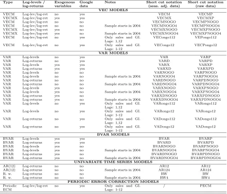
data. The full details of all 34 multivariate models are reported in Table 7. For ease of reference, we

also report in the sixth column a short-cut notation for identifying each model in the tables reporting

the models forecasting performances.

We used the data between 2001M1 and 2008M9 as the first initialization sample for the models

without Google data, and data from 2004M1 till 2008M9 for the models with Google data and those

without Google data but estimated on a shorter sample. The evaluation period ranged from 2008M10

till 2014M6 and was used to compare forecasts from 1 step ahead up to 24 steps ahead. The top three

models in terms of the Mean Squared Prediction Error (MSPE) for each forecasting horizon and each

car brand are reported in Table 15, while the full results are available from the authors upon request.

Table 15 shows that there is no single model which outperforms all competitors for all horizons and

all car brands. However, some general indications can be retrieved:

•

The MSPEs of the competing models with forecasting horizons up to 8-10 steps ahead are relatively

(14)

Type

Log-levels /

Exogenous

Google

Notes

Short cut notation

log-returns

variables

data

(seas. adj. data)

(raw data)

VEC MODELS

VECM

Log-lev/log-ret

no

yes

VECM

VECMP

VECMX

Log-lev/log-ret

yes

VECMX

VECMXP

VECM

Log-lev/log-ret

no

VECMNOGO

VECMPNOGO

VECM

Log-lev/log-ret

no

Sample starts in 2004

VECMNOGO4

VECMPNOGO4

VECMX

Log-lev/log-ret

yes

no

VECMXNOGO

VECMXPNOGO

VECMX

Log-lev/log-ret

yes

no

Sample starts in 2004

VECMXNOGO4

VECMXPNOGO4

VECM

Log-lev/log-ret

no

yes

Only sales and GI.

Lags: 1,12

VECongo112

VEPongo112

VECM

Log-lev/log-ret

no

yes

Only sales and GI.

Lags: 1-12

VECongo12

VECPongo12

VAR MODELS

VAR

Log-levels

no

yes

VAR

VARP

VAR

Log-returns

no

yes

VARD

VARPD

VAR

Log-levels

yes

VARX

VARXP

VAR

Log-returns

yes

VARXD

VARXPD

VAR

Log-levels

no

VARNOGO

VARPNOGO

VAR

Log-levels

no

VARNOGO4

VARPNOGO4

VAR

Log-returns

no

VARDNOGO

VARPDNOGO

VAR

Log-returns

no

VARDNOGO4

VARPDNOGO4

VAR

Log-levels

yes

no

VARXNOGO

VARXPNOGO

VAR

Log-levels

yes

no

VARXNOGO4

VARXPNOGO4

VAR

Log-returns

yes

no

VARXDNOGO

VARXPDNOGO

VAR

Log-returns

yes

no

Sample starts in 2004

VARXDNOGO4

VARXPDNOGO4

VAR

Log-levels

no

yes

Only sales and GI.

Lags: 1,12

VARongo112

VAR

Log-levels

no

yes

Only sales and GI.

Lags: 1-12

VARongo12

VAR

Log-returns

no

yes

Only sales and GI.

Lags: 1,12

VADongo112

VAR

Log-returns

no

yes

Only sales and GI.

Lags: 1-12

VADongo12

BVAR MODELS

BVAR

Log-levels

yes

BVAR

BVARP

BVAR

Log-returns

yes

BVARD

BVARPD

BVAR

Log-levels

yes

no

BVARNOGO

BVARPNOGO

BVAR

Log-levels

yes

no

BVARNOGO4

BVARPNOGO4

BVAR

Log-returns

yes

no

BVARDNOGO

BVARPDNOGO

BVAR

Log-returns

yes

no

BVARDNOGO4

BVARPDNOGO4

UNIVARIATE TIME SERIES MODELS

AR(12)

Log-returns

no

AR12

AR(12)

Log-returns

no

AR124

R. w.

Log-returns

no

RW

R. w.

Log-returns

no

RW4

PERIODIC ERROR CORRECTION MODELS

Periodic

ECM

Log-lev/log-ret

no

yes

Only sales and GI.

Lags: 1-12

[image:14.612.72.539.38.438.2]

/

PECM

Table 7: Models used for forecasting (baseline case).

•

Bayesian VAR models, particularly in differences and without Google data, perform rather well

across all car brands and for short and medium forecasts (up to 12 steps ahead);

•

Bivariate models including only car sales and Google models and using only the first and the 12th

lags perform extremely well across most of the car brands examined, particularly for long-term

forecasts. The parsimonious specifications of these models clearly allow for efficiency gains where

forecasting is of concern.

•

The forecasting power of the best models using Google data increases with the length of the forecast

horizon, particularly with forecast horizons higher than 12 steps ahead. This evidence is similar to

that found in D’Amuri and Marcucci (2013) and Fantazzini and Fomichev (2014).

•

Models without Google data estimated with the long sample starting in 2001 tend to perform better

than those estimated with a shorter sample starting in 2004.

•

There are no particular differences between large, medium-sized and small sellers and between

foreign and German manufacturers.

(15)

model without Google data and the Random Walk model. We remark that the best models tend to vary

across different horizons.

0.0 0.2 0.4 0.6 0.8 1.0

5 10 15 20

BMW: MODEL WITH GI BMW: MODEL WITHOUT GI

0.0 0.2 0.4 0.6 0.8 1.0

5 10 15 20

CITROEN: MODEL WITH GI CITROEN: MODEL WITHOUT GI

SEASONALLY ADJUSTED DATA

0.0 0.2 0.4 0.6 0.8 1.0 1.2

5 10 15 20

FIAT: LINEAR WITH GI FIAT: LINEAR WITHOUT GI

0.0 0.2 0.4 0.6 0.8 1.0

5 10 15 20

JAGUAR: MODEL WITH GI JAGUAR: MODEL WITHOUT GI

0.0 0.2 0.4 0.6 0.8 1.0 1.2

5 10 15 20

KIA: MODEL WITH GI KIA: MODEL WITHOUT GI

0.0 0.2 0.4 0.6 0.8 1.0

5 10 15 20

MITSUBISHI: MODEL WITH GI MITSUBISHI: MODEL WITHOUT GI

0.0 0.2 0.4 0.6 0.8 1.0

5 10 15 20

OPEL: MODEL WITH GI OPEL: MODEL WITHOUT GI

0.0 0.2 0.4 0.6 0.8 1.0 1.2

5 10 15 20

SUZUKI: MODEL WITH GI SUZUKI: MODEL WITHOUT GI

0.0 0.2 0.4 0.6 0.8 1.0 1.2

5 10 15 20

TOYOTA: MODEL WITH GI TOYOTA: MODEL WITHOUT GI

0.0 0.2 0.4 0.6 0.8 1.0

5 10 15 20

VOLKSWAGEN: MODEL WITH GI VOLKSWAGEN: MODEL WITHOUT GI

SEASONALLY ADJUSTED DATA

0.0 0.2 0.4 0.6 0.8 1.0

5 10 15 20

BMW: MODEL WITH GI BMW: MODEL WITHOUT GI

0.0 0.2 0.4 0.6 0.8 1.0

5 10 15 20

CITROEN: MODEL WITH GI CITROEN: MODEL WITHOUT GI

0.0 0.2 0.4 0.6 0.8 1.0 1.2

5 10 15 20

FIAT: MODEL WITH GI FIAT: MODEL WITHOUT GI

0.0 0.2 0.4 0.6 0.8 1.0

5 10 15 20

JAGUAR: MODEL WITH GI JAGUAR: MODEL WITHOUT GI

0.0 0.2 0.4 0.6 0.8 1.0 1.2

5 10 15 20

KIA: MODEL WITH GI KIA: MODEL WITHOUT GI

0.0 0.2 0.4 0.6 0.8 1.0 1.2

5 10 15 20

MITSUBISHI: MODEL WITH GI MITSUBISHI: MODEL WITHOUT GI

0.0 0.2 0.4 0.6 0.8 1.0 1.2

5 10 15 20

OPEL: MODEL WITH GI OPEL: MODEL WITHOUT GI

0.0 0.2 0.4 0.6 0.8 1.0

5 10 15 20

SUZUKI: MODEL WITH GI SUZUKI: MODEL WITHOUT GI

0.0 0.2 0.4 0.6 0.8 1.0

5 10 15 20

TOYOTA: MODEL WITH GI TOYOTA: MODEL WITHOUT GI

0.0 0.2 0.4 0.6 0.8 1.0

5 10 15 20

VOLKSWAGEN: MODEL WITH GI VOLKSWAGEN: MODEL WITHOUT GI

[image:15.612.81.530.91.534.2]

RAW DATA RAW DATA

Figure 4: Ratios of the MSPEs of the best models with and without Google data and the Random Walk

model across all forecasting horizons. The first two columns show results for seasonally-adjusted data,

and the last two for raw data.

(16)

Model rankings in terms of the MSPE do not show whether the competing forecasts are statistically

different or not. We therefore tested for significant differences in forecast accuracy using the Model

Confi-dence Set (MCS) approach proposed by Hansen, Lunde, and Nason (2011). The MCS is a sequential test

of equal predictive ability, with the starting hypothesis that all models considered have equal forecasting

performance. Given an initial set of forecasts, it tests the null that no forecast is distinguishable from

any other and discards any inferior forecasts if they exist. The MCS procedure yields a model confidence

set containing the best forecasting models at a given confidence level. Since our dataset is not too large

and the number of forecasting models is moderate, we employed the semiquadratic test statistic (

T

SQ

),

which is more computationally intensive but more selective, see e.g. Rossi and Fantazzini (2014). The

loss function used was the MSPE, while the

p

-values for the test statistic were obtained using a stationary

block bootstrap with a block length of 12 months and 1000 re-samples. If the

p-value was lower than a

defined confidence level

α, the model was not included in the MCS and viceversa. A brief description of

the MCS approach is reported in the Technical Appendix F.

The models included in the MCS at the 10% level for all car brands and forecast horizons are reported

in Table 16

4

: for the sake of space and interest, we report only the total number of selected models, the

total number of selected Google-based models, and whether the Random Walk model was included or

not. The full set of results is available from the authors upon request.

Table 16 shows that most, if not all, models are selected in the case of forecasts up to 10-12 steps

ahead for five car brands out of ten: the differences in forecasting performances are not large enough

to distinguish between them, meaning that the MCS contains a large number of models. Moreover, the

Random Walk model is often included. Instead, for long-term forecasts (12 steps ahead and higher),

only a small number of models is selected, most of them bivariate models including only car sales and

GIs, Bayesian VARs with GIs and sometimes the AR(12). Besides, the Random Walk model is seldom

included. Here, the data are much more informative and it is possible to select a limited number of

models which statistically outperform their competitors.

3.2

Raw data

We compared the same 34 models used for seasonally-adjusted data, but augmented with centered

seasonal dummies to model potential seasonal behavior. Moreover, we also considered the bivariate

Periodic Error Correction Model PECM(1,12) which includes only car sales and Google data, as discussed

in section 2.2.2. To account for the possible endogeneity of regressors and improve the efficiency of the

parameter estimates in small samples, we estimated the error correction term using the method of

dynamic OLS (see Boswijk and Franses (1995), Hayashi (2000) and Franses and Paap (2004)). A

short-cut notation for identifying each model in the subsequent tables reporting their forecasting performances

is reported in the last column of Table 7.

We used the data between 2001M1 and 2009M6 as the first initialization sample for the models without

Google data, while we used the initialization sample 2004M1-2009M6 for the models with Google data

and for those without Google data but estimated on a shorter sample. The evaluation period ranged from

2009M7 till 2014M6 and was used to compare forecasts from 1 step ahead up to 24 steps ahead. The top

three models in terms of the Mean Squared Prediction Error (MSPE) for each forecasting horizon and

each car brand are reported in Table 17, while a summary of the models included in the MCS is reported

in Table 18. The ratios of the MSPE of the best model with Google data and the Random Walk model

across all forecasting horizons, together with the ratios of the MSPE of the best model without Google

data and the Random Walk model are shown in the last two columns of Figure 4.

The results are somewhat similar to those which emerged from seasonally-adjusted data, but there are

also some important differences. Models without Google data now perform better, with respect to the case

of seasonally-adjusted data. Moreover, the number of models selected in the MCS is now much smaller

(often no more than 2-6 models): Bayesian VARs (with and without Google data) and parsimonious

bivariate models including only sales and GIs again represent the majority of models included in the

MCS at the 10% level.

(17)

4

Robustness Checks

We wanted to verify that the superior performance of Google-based models also holds under alternative

forecasting. We performed a series of robustness checks, considering alternative nonlinear models,

alter-native out-of-sample intervals, evaluating the directional accuracy of the competing forecasting models,

checking whether Google data downloaded on different days can affect the models’ forecasting

perfor-mances, and examining additional car brands.

4.1

Nonlinear Models

A part of the economic and financial literature has suggested the use of nonlinear models for forecasting

purposes (for instance, see Franses and Dijk (2000) and Terasvirta, Tjostheim, and Granger (2011) for

a discussion at the textbook level). Given this evidence, we estimated a set of nonlinear models and

compared their forecasting performances with the models in section 3. More specifically, we considered

three nonlinear models:

•

the SETAR model with 2 regimes (see Tong (1990) for a discussion at the textbook level);

•

the logistic smooth transition autoregressive (LSTAR) model, which is a generalization of the

SETAR model (see Tong (1990));

•

the additive autoregressive model (AAR), also known as generalized additive model (GAM), since

it combines generalized linear models and additive models (see Wood (2006) for a discussion at the

textbook level).

A description of these nonlinear models is given in the Technical Appendix G. See D’Amuri and Marcucci

(2013) and Fantazzini and Fomichev (2014) for a discussion of robustness checks using these nonlinear

models.

The top three models in terms of the MSPE for each forecasting horizon and each car brand are

reported in Table 19 for seasonally-adjusted data and in Table 21 for raw data. A summary of the

models included in the MCS is reported in Table 20 for seasonally-adjusted data and in Table 22 for raw

data.

In general, nonlinear models are very competitive, thus confirming past literature dealing with car

sales forecasting (see Da, Engelberg, and Pengjie (2003), Kunhui, Qiang, Changle, and Junfeng (2007),

Br¨

uhl, Borscheid, Friedrich, and Reith (2009), Hulsmann, Borscheid, Friedrich, and Reith (2012)).

Par-ticularly, parsimonious AAR and SETAR models involving only a few lags are often ranked among the

top models in terms of MSPE. Moreover, AAR models with log-prices performed very well for

medium-and long-term forecasts, similarly to what was found in Fantazzini medium-and Fomichev (2014) when

forecast-ing the real price of oil. However, nonlinear models were difficult to estimate, and specifications with

a large number of lags failed to converge. Particularly, the LSTAR proved to be the most challenging

and computationally intensive (see Franses and Dijk (2000) for a discussion of this issue). The results of

the MCS confirm this evidence and most of the models included at the 10% level are nonlinear, whereas

the only selected linear models are mostly Google-based. This evidence therefore seems to suggest that

Google data may explain a good portion of the nonlinearity displayed by sales data.

In the case of raw data, nonlinear models are less competitive than linear models, particularly for

forecasting horizons up to 12 steps ahead, whereas Bayesian VAR models and bivariate linear models

including car sales and GIs are often the top ranked models across most of the car brands. However, for

long-term forecasts, more than half of the models included in the MCS are nonlinear, while the remaining

selected models are mainly bivariate Google-based models.

(18)

SEASONALLY ADJUSTED DATA

Bmw Citroen Fiat Jaguar Kia

Model MSE Ranking MCS Model MSE Ranking MCS Model MSE Ranking MCS Model MSE Ranking MCS Model MSE Ranking MCS

Linear w. GI BVAR 7255188 36 Yes VARD 1937867 4 Yes VARongo112 11439630 10 Yes VADongo112 7409 22 Yes VARongo112 1220217 18 Yes Linear w/o GI AR12 6080991 4 Yes VARDNOGO 2054348 6 No BVARNOGO 11763929 11 Yes AR12 6913 11 Yes AR12 1036132 12 Yes Nonlinear AAR(7)dlog 5698093 1 Yes LSTAR(3)log 1688104 1 Yes SETAR(2)log 9458281 1 Yes SETAR(5)log 6478 1 Yes AAR(4)log 909397 1 Yes

RW 9073312 54 Yes 2534232 36 No 13839395 26 Yes 8907 61 Yes 1406331 28 Yes

Mitsubishi Opel Suzuki Toyota Volkswagen

Linear w. GI VECongo112 285910 1 Yes VECongo112 16265040 1 Yes VARongo112 1206941 9 Yes VECongo112 4040621 1 Yes VARongo112 60790600 2 Yes Linear w/o GI VECMNOGO4 484285 32 Yes VECMXNOGO 21934786 6 No VECMXNOGO 1233267 10 Yes VECMXNOGO 5429724 3 Yes AR124 58970200 1 Yes Nonlinear SETAR(11)log 347695 3 Yes AAR(2)log 24373967 9 No SETAR(3)log 812440 1 Yes AAR(1)log 5653546 6 Yes AAR(1)log 71730620 9 No

RW 577041 62 Yes 36590894 40 No 1760865 27 No 7663277 29 No 94350150 36 No

RAW DATA

Linear w. GI VADongo112 9546849 1 Yes VARongo112 913022 3 Yes VARongo112 1225557 1 Yes BVARPD 7852 1 Yes BVARPD 731755 1 Yes Linear w/o GI BVARPDNOGO10099266 2 Yes BVARPNOGO 763696 1 Yes BVARPNOGO 2874716 13 Yes BVARPDNOGO4 8209 2 Yes BVARPDNOGO753717 3 Yes Nonlinear AAR(8)log 17435149 24 No AAR(3)log 1121818 6 No LSTAR(2)log 2615865 2 Yes AAR(3)log 12342 30 No AAR(9)log 828305 6 Yes

RW 21780883 62 No 3800014 70 No 9377139 62 No 15886 90 No 1218423 33 No

Linear w. GI VEPongo112 193905 1 Yes VEPongo112 11342673 1 Yes BVARP 523703 12 Yes VEPongo112 3433042 2 Yes VEPongo112 48248128 2 Yes Linear w/o GI BVARPDNOGO322456 26 Yes BVARPNOGO 15033303 5 No BVARPNOGO4 380224 10 Yes VECMXPNOGO4 3333000 1 Yes BVARPNOGO 45734023 1 Yes Nonlinear LSTAR(3)log 234530 2 Yes SETAR(9)dlog 31266013 29 No SETAR(2)log 269229 1 Yes SETAR(1)dlog 4165033 6 Yes SETAR(4)log 72437319 12 No

[image:18.792.77.778.95.280.2]

RW 319260 24 Yes 34959425 38 No 1244803 34 No 5758188 30 No 153257703 63 No

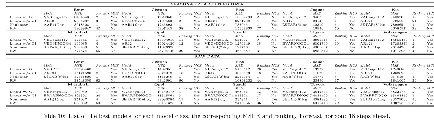
Table 8: List of the best models for each model class, the corresponding MSPE and ranking. Forecast horizon: 6 steps ahead.

SEASONALLY ADJUSTED DATA

Linear w. GI VARongo112 11630497 20 Yes VECongo112 1746615 9 Yes VARongo112 8070599 15 No VECongo112 9089 15 Yes VARongo112 1226001 24 Linear w/o GI AR12 9491265 5 Yes BVARNOGO 1302593 6 Yes BVARNOGO 5773194 10 No AR12 8158 3 Yes AR12 859701 14 Nonlinear SETAR(1)log 8506115 1 Yes SETAR(4)log 1170021 1 Yes AAR(1)log 2142114 1 Yes SETAR(3)log 7758 1 Yes SETAR(3)log 709664 1

RW 13909104 43 Yes 3606090 43 No 14889930 30 No 13024 63 Yes 1830155 29

Linear w. GI VECongo12 227696 1 Yes VECongo112 21470315 3 Yes BVAR 921548 12 No BVAR 5198460 6 Yes VARongo112 34715966 2 Yes Linear w/o GI AR12 446751 5 Yes BVARNOGO 22609378 5 Yes BVARNOGO4 979593 14 No BVARNOGO4 4832954 1 Yes AR124 28352989 1 Yes Nonlinear SETAR(11)log 393336 12 Yes SETAR(7)dlog 20607165 1 Yes AAR(3)log 222809 1 Yes SETAR(7)dlog 4977505 2 Yes SETAR(7)log 37548975 4 Yes RW 888768 70 Yes 37088135 43 No 3319004 44 No 10675830 36 No 133013321 47 No

RAW DATA

Linear w. GI VADongo112 11298025 3 Yes VARongo112 872250 1 Yes PECM 2688297 15 Yes BVARPD 9021 2 Yes VADongo112 859092 3 Yes Linear w/o GI AR124 11133748 1 Yes AAR(3)log 1109012 3 Yes BVARPNOGO4 3686731 23 No BVARPDNOGO4 8749 1 Yes BVARPDNOGO871338 5 Yes Nonlinear SETAR(10)log 13316723 9 No BVARPNOGO 1156313 4 Yes SETAR(1)log 1732960 1 Yes SETAR(7)dlog 11973 13 Yes AAR(9)log 765639 1 Yes

RW 15260733 16 No 2734442 47 No 3822802 24 Yes 11294 9 Yes 942287 10 Yes

Linear w. GI VEPongo112 207765 1 Yes VEPongo112 12940989 1 Yes BVARP 585175 13 No VEPongo112 2398770 1 Yes BVARP 78930479 7 Yes Linear w/o GI AR12 414701 26 Yes BVARPNOGO 19896671 4 No BVARPNOGO4 541203 12 Yes BVARPDNOGO4 3334235 6 Yes BVARPNOGO 60857150 1 Yes Nonlinear AAR(1)log 273074 2 Yes AAR(1)dlog 24701172 13 No AAR(4)log 240509 1 Yes SETAR(6)log 3292246 5 Yes SETAR(6)log 72922923 2 Yes

RW 493513 41 Yes 18710646 3 Yes 1613001 38 No 4803964 26 No 98132979 22 Yes

Table 9: List of the best models for each model class, the corresponding MSPE and ranking. Forecast horizon: 12 steps ahead.

[image:18.792.74.792.302.475.2]

(19)

SEASONALLY ADJUSTED DATA

Linear w. GI VARongo112 8464643 2 Yes VECongo112 1920350 7 Yes VECongo112 13037790 21 No VECongo112 9462 2 Yes VARongo112 940676 19 Yes Linear w/o GI AR12 9384237 3 Yes BVARNOGO 2109563 9 Yes AR124 2271788 4 Yes AR12 9313 1 Yes AR124 970566 21 Yes Nonlinear AAR(1)log 8018508 1 Yes AAR(1)log 1266893 1 Yes AAR(1)log 783045 1 Yes LSTAR(5)log 10319 6 Yes SETAR(8)log 780965 1 Yes

RW 19689847 42 No 4907445 38 No 15368830 27 No 16920 50 No 2358597 29 No

Linear w. GI VECongo112 174546 1 Yes VECongo112 18394010 11 Yes VARongo112 634907 9 No VECongo112 3866818 1 Yes VARongo112 14865460 1 Yes Linear w/o GI VECMNOGO4 195035 4 Yes AR12 19024430 12 Yes VECMXNOGO 1279649 15 No BVARNOGO4 6302790 19 Yes AR124 17283870 2 Yes Nonlinear SETAR(10)log 288480 5 No SETAR(7)dlog 11826920 1 Yes SETAR(2)log 191776 1 Yes SETAR(3)dlog 4001607 2 Yes AAR(1)log 26144200 4 Yes

RW 777574 66 No 25704740 29 Yes 4680547 37 No 9851512 36 No 107189500 43 No

RAW DATA

Linear w. GI VARPD 15598460 11 Yes VARongo112 1402351 2 Yes VEPongo112 5156512 20 Yes VEPongo112 13929 2 Yes VEPongo112 1249080 5 Yes Linear w/o GI AR124 15171520 8 Yes BVARPNOGO 2374012 15 Yes AR12 4056693 18 Yes VARPNOGO 11879 1 Yes AR124 1262323 6 Yes Nonlinear LSTAR(9)log 12761820 1 Yes AAR(3)log 1151259 1 Yes LSTAR(2)log 2217764 1 Yes AAR(3)log 14774 4 Yes AAR(9)log 967518 1 Yes

RW 38548350 62 No 6342691 66 No 10898232 44 No 23496 67 Yes 1841665 29 No

Linear w. GI VEPongo112 159969 1 Yes VARongo112 10159473 1 Yes VARongo112 463961 13 Yes VEPongo112 3849544 1 Yes VECPongo12 58221750 2 Yes Linear w/o GI BVARPNOGO4 395301 24 Yes BVARPDNOGO 18345564 3 Yes BVARPNOGO4 816324 17 No BVARPDNOGO4438429 6 Yes BVARPNOGO 55863450 1 Yes Nonlinear AAR(1)