Munich Personal RePEc Archive
Monetary Policy and Large Crises in a
Financial Accelerator Agent-Based
Model
Giri, Federico and Riccetti, Luca and Russo, Alberto and
Gallegati, Mauro
Università Politecnica delle Marche, La Sapienza Università di Roma
30 March 2016
Online at
https://mpra.ub.uni-muenchen.de/70371/
Monetary Policy and Large Crises in a
Financial Accelerator Agent-Based Model
Federico Giri
∗1, Luca Riccetti
2, Alberto Russo
1, and Mauro
Gallegati
11
Universit`a Politecnica delle Marche, Ancona, Italy
2Sapienza Universit`a di Roma, Roma, Italy
March 30, 2016
Abstract
An accommodating monetary policy followed by a sudden increase of the short term interest rate often leads to a bubble burst and to an economic slowdown. Two examples are the Great Depression of 1929 and the Great Recession of 2008. Through the implementation of an Agent Based Model with a financial accelerator mechanism we are able to study the relationship between monetary policy and large scale crisis events. The main results can be summarized as follow: a) sudden and sharp increases of the policy rate can generate recessions; b) after a crisis, returning too soon and too quickly to a normal monetary policy regime can generate a “double dip” recession, while c) keeping the short term interest rate anchored to the zero lower bound in the short run can successfully avoid a further slowdown.
Keywords: Monetary Policy, Large Crises, Agent Based Model, Financial Accelerator, Zero Lower Bound .
JEL classification codes: E32, E44, E58, C63.
Po-1
Introduction
As highlighted by Fratianni and Giri (2015), monetary policy played a non
negligible role in both the largest disruptive events of the 20th century, the
Great Depression of 1929 and the Great Recession of 2008. The combination
of a long-lasting accommodating monetary policy just followed by a sharp and
quick monetary contraction results to be a powerful destabilizing mechanism.
To support this view, Taylor (2009, 2007) compared the behavior of the
monetary policy conducted by the Federal Reserve and the predicted values
implied by a simple Taylor rule.
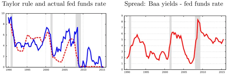
Figure 1 shows that, during the period 2001-2004, the fed funds rate was
well below, almost 300 basis points at the end of 2004, the value predicted
using a standard Taylor rule (see Taylor, 1993). This part of the decade
is usually referred as the “Greenspan put”, that is a period of exceptionally
low interest rates and expansionary monetary policy under the Fed chairman
Alan Greenspan.
The reason of such an aggressive expansionary monetary policy can be
traced back to the burst of the “dot com” bubble in 2000-2001. The following
recession forced the Federal Reserve to take drastic measures in order to
restore the normal functioning of the US economy.
Credit provided by financial intermediaries to buy new houses became
cheaper, fueling a bubble on the housing market (see Bordo and
Landon-Lane, 2013, and Ferrero, 2015). At the end of 2004, the concerns about
a possible resurgence of inflation convinced the governor of the Fed, Ben
Bernanke, to abandon the accommodating monetary policy started by his
predecessor. He increased the fed funds rate sharply from a value slightly
above 1 % to a new one of 5.25 % in less than two years.
Figure 1
Taylor rule and actual fed funds rate Spread: Baa yields - fed funds rate
0 1 2 3 4 5 6 7 8 9
1990 1995 2000 2005 2010 2015
Source: FRED database and authors calculations. Left graph: the expression of the Taylor rule is taken from Taylor (1993). itr=max{0,4% + 1.5(πt−2%) + 0.5ye}. The red dashed line represents the effective fed funds rate, the blue line are the values predicted according to the Taylors rule. Grey bars represent recessions according to the NBER classification.
an increase of the interest rates on loans to firms. Following Gilchrist and
Zakrajsek (2012), we calculate and report in Figure 1 the spread between
the Baa corporate bond yields and the effective Fed funds rate. The cost of
external funding rose of more than 8 % during the 2007 financial crisis with
respect to the risk free rate.
The main consequence in 2008 of this combination of events was the burst
of the sub-prime mortgages crisis (and, consequently, the end of the expansion
Monetary policy after the Great Recession changed radically and it was
characterized by extreme monetary policy measures that pushed the
inter-est rates closed to the zero lower bound of interinter-est rates (henceforth ZLB).
Moreover, once the ZLB was reached and the effectiveness of monetary
pol-icy based on steering the short term interest rates was undermined, central
banks began to experiment unexplored way to stimulate the economy.1
The aim of this paper is to provide answers to three important questions:
a) is there a macroeconomic relationship between monetary policy and large
scale crisis events? b) Is the so called “Forward Guidance” of short term
interest rates an effective tools of unconventional monetary policy? c) After
a crisis, should the conduction of monetary policy return to a normal
imple-mentation as soon as possible or is it desirable to keep the interest rates close
to the ZLB for an extended period of time?
In order to do that, we built an Agent Based Macroeconomic model
(henceforth ABM) with interacting agents including a financial accelerator
mechanism as in Bernanke et al. (1999), that is the standard mechanism to
introduce financial frictions in the classical DSGE models.
Why do we use an ABM model? Following Quadrini (2011), heterogeneity
is an essential element of every DSGE model with financial intermediaries,
but taking into account the entire distribution of agents became a daunting
task as soon as the model is enriched along several dimensions. The most
common shortcut in the mainstream literature is to assume the existence
of two representative heterogeneous agents, borrowers and savers, like in
1
Kiyotaki and Moore (1997). Alternatively, one can assume the existence of a
continuum of agents (like in Bernanke et al. (1999) and Carlstrom and Fuerst
(1997)). The behavior of such agents can be summarized by a single equation
thank to the linear aggregation (Quadrini, 2011, p 215). Implementing the
financial accelerator framework into an ABM seems to be a natural extension
of such models.
Moreover, ABMs have been already used as computational tools to
inves-tigate economic policy issues in a macroeconomic framework: for instance,
Delli Gatti et al. (2005) explore the role of monetary policy in a complex
sys-tem with agent’s learning; Russo et al. (2007) focus on fiscal policy and its
effect on R&D dynamics; Haber (2008) investigates the effect of both fiscal
and monetary policies; Cincotti et al. (2010, 2012a) investigate the causes of
macroeconomic instability and, in particular, the role of deleveraging;
Babut-sidze (2012) analyzes the implications for monetary policy of price-setting;
Cincotti et al. (2012b) analyze the role of banking regulation finding that
both unregulated financial systems and overly restrictive regulations have
destabilizing effects; Dosi et al. (2013) consider the interplay between
in-come distribution and economic policies; Salle et al. (2013) focus on inflation
targeting; Dosi et al. (2015) evaluate the effect of both fiscal and monetary
policy in complex evolving economies; da Silva and Lima (2015) studies the
interplay between the monetary policy rate and financial regulation; Krug
et al. (2015) evaluate the impact of Basel III on financial instability; Ashraf
et al. (2016) analyze the impact of the trend rate of inflation on
macroeco-nomic performance; Riccetti et al. (2016) explore the effects of banking
reg-ulation on financial stability and endogenous macroeconomic crises. All in
all, ABMs represent an alternative approach for studying a complex
(Dawid and Neugart, 2011).2
Another fundamental issue is the way in which financial factors are
in-cluded into a macroeconomic model that is strictly related to the problem
of replicating, at least qualitatively, the dynamic evolution of the spread
between the lending rates and the policy rate.
DSGE models literature focuses its attention on two different approaches
to include financial factors into general equilibrium set up, the collateral
con-straint like in Kiyotaki and Moore (1997) and the already mentioned financial
accelerator mechanism like in Bernanke et al. (1999). The first approach
fo-cuses its attention on the importance of collateral provided by the borrowers
that cannot receive a loans for an amount larger than the expected value of
their collaterals, typically physical capital or housing services. Instead, the
financial accelerator mechanism boils down from a costly state verification
problem. Monitoring a loan is costly for financial intermediaries forcing them
to apply a spread over the risk free interest rate, the so called external risk
premium.
We decide to include in our ABM a financial accelerator mechanism for
two main reasons. The first is a modeling choice since, as we previously
stated, the financial accelerator can be naturally extended in a framework
with heterogeneous agents. The second motivation is empirical. The financial
accelerator seems to perform better with respect to the collateral constraint
set up in order to reproduce the same stylized facts like volatilities and hump
shape responses of the same variables of interest (Brzoza-Brzezina et al.,
2013).
The main findings of our contribution are the followings: a) An increase
of short term interest rates can generate a large scale crisis if the increase
2
happens too quickly and too sharply; b) after a crisis, if the central bank
returns too early to conduct monetary policy steering the short term interest
rates, the possibility of falling in a “double dip” recession is significant, while
c) keeping short term interest rates close to the zero lower bound helps the
central bank to stabilize the economy, at least in the short run.
The paper is organized as follow: Section 2 presents the ABM model in
details, while Section 3 shows the general properties of the model, the
de-scriptions of a large scale crisis events produced by the model and a
counter-factual unconventional monetary policy experiments. Section 4 summarizes
the main findings and the possible future developments of this work.
2
The model
In this section we provide a description of the ABM we propose to analyze
macroeconomic dynamics and, in particular, the behavior of the monetary
authority during large crisis events. It is worth to notice that model dynamics
are not limited to the relationship between monetary policy and recessions.
Indeed, the model is able to endogenously reproduce a variety of
macroe-conomic scenarios and different typology of crises, such as crises due to real
factors. Our choice in this paper is, however, to focus on the particular nexus
between the central bank’s behavior and the evolution of crises.
In what follows, firstly, we present the set up of the model; secondly, we
describe the sequence of events occurring in our economy; then, we provide
2.1
Model setup
The economy evolves over a time span t = 1,2, ..., T and it is composed of
households (h = 1,2, ..., H), capital goods firms (k = 1,2, ..., K),
consump-tion goods firms (f = 1,2, ..., F), a banking system, a central bank, and the
government. Agents are boundedly rational and live in an incomplete and
asymmetric information context, thus they follow simple rules of behavior
and use adaptive expectations. For the sake of simplicity, we assume that
consumption goods are produced by means of capital goods and that capital
goods are produced only by employing labor. This simplifying assumption
allows us to border the direct interaction between firms and workers in the
labor market to one typology of firms, that is capital goods producers.
Al-though this may lead to a certain loss of realism, for instance resulting in a
higher volatility of unemployment, it does not prevent the model to
quali-tatively explain various characteristics of the business cycles. Moreover, we
focus more on financial aspects, as the dynamics of interest rates’ spread,
than on the level of unemployment.3
Agents interact in five markets: credit, labor, investment goods,
con-sumption goods and deposits. The first and the last market in the previous
list are not based on a decentralized mechanism, while in other markets the
interaction mechanism that matches the demand and the supply sides follows
a common decentralized matching protocol (Riccetti et al., 2015). In
particu-lar, the interaction process develops as follows: a random list of agents on the
demand side is set, then the first agent on the list observes a random subset
of potential counterparts on the supply side, the size of which depends on a
parameter 0< χ≤1 (that proxies the degree of imperfect information), and
3
chooses the cheapest one. After that, the second agent on the list performs
the same activity on a new random subset of the updated potential partner
list. The process iterates until the end of the demand side list. Subsequently,
a new random list of agents in the demand side is set and the whole matching
mechanism continues until either one side of the market (demand or supply)
is empty or no further matchings are feasible because the highest bid (for
example, the money available to the richest firm) is lower than the lowest
ask (for example, the lowest wage asked by unemployed workers).
2.2
Sequence of events
The sequence of events runs as follows.
• At the beginning of each period, new entrants substitute bankrupted
agents according to a one-to-one replacement.4
• The capital used by consumption goods producers depreciates.
• Firms set their desired production based on past production, expected
profitability and the level of inventories.
• Based on desired production and given the expected price of capital,
consumption goods producers derive total financing; the demand for
credit is then given by total financing less net worth plus the possible
outstanding debt.
4
• Based on desired production, capital producers set their labor demand;
the resulting demand for credit is given by the expected wage bill
mi-nus internal resources plus the possible outstanding debt previously
received.
• The credit market opens: the demand of credit comes from both capital
and consumption goods producers; the supply of credit is set by the
banking system as a multiple of its net worth; in particular, credit
supply increases (decreases) as the bank’s profit increases (decreases);
in the case the demand is higher than the supply, firms are credit
rationed proportionally. Firms’ liquidity is then given by both internal
and external resources.
• The bank sets interest rates by charging a risk premium on firm loans
which gives rise to the financial accelerator mechanism.
• Insolvent as well as illiquid firms are declared bankrupted; the banking
system suffers non-performing loans for the fraction of loans not repaid
by firms; moreover, the bank comes into the possession of firms’
inven-tories of capital and consumption goods, respectively, that it tries to
sell at a discounted price in the respective markets.
• The labor market opens: employed workers get their wage on which
they pay a proportional tax; the unemployment rate can be computed;
some vacancies may remain unfulfilled due to both mismatch between
the supply and the demand of labor and a lack of aggregate demand.
• Workers update their desired wage: upwards if employed, downwards
otherwise; however, the desired wage has a lower bound tied to the
• Capital goods are produced by employing the hired workers; current
production plus inventories is available on the market to be sold to
consumption goods producers.
• The capital goods market opens and a decentralized matching between
firms takes place; due to both a lack of demand and supply/demand
mismatch, some capital goods may remain unsold and then considered
as inventories.
• Consumption goods are produced by employing capital goods; current
production plus inventories is available on the market to be sold to
households.
• The consumption goods market opens and a decentralized matching
between firms and households takes place: due to both a lack of demand
and supply/demand mismatch, some consumption goods may remain
unsold and then considered as inventories.
• Firms update their selling prices.
• Households’ saving is deposited in the banking system and gives rise
to the payment of an interest on which depositors pay a proportional
tax; households also pay a wealth tax according to a proportional tax
rate.
• The public deficit and the public debt is computed.
• Government securities are bought by the banking sector; in the case
the private demand for these bonds is below the supply, the central
• Depending on the balance sheet of the banking sector, the central bank
either provides money injection or receives reserves.
• Firms compute their profits on which they pay a proportional tax
(neg-ative profits are subtracted from the tax that the firm should pay on
next positive profits); a fraction of net profits is distributed as dividends
to households (proportionally to their relative wealth); then, firms’ net
worth is updated.
• In the case firms’ liquidity is negative, they decide to ask a bank loan
to cover it (if in the next period they do not receive such a loan, they
go bankrupt).
• The banking sector computes its profit on which it pays a proportional
tax (negative profits are subtracted from the tax that the bank should
pay on next positive profits); a fraction of the net profit is distributed
as dividends to households (proportionally to their relative wealth);
then, the net worth of the banking sector is updated.
• Aggregate variables are computed.
• The central bank sets the policy rate for the next period according to
the Taylor rule.
In next subsections, we describe in more detail the behavior of agents and
the specific structure of different markets.
2.3
Consumption goods producers
Firms that produce consumption goods use capital goods as the only factor
depre-ciates at the rate δ. Consequently, the number of capital goods of the firm
f at the beginning of period t is:5
x′
f t=
(1−δ)x′′
f t−1
(1)
wherex′′
f t−1 represents the capital goods already owned by the firm.
6
The desired level of sales for consumption goods producers depends on
past sales, profits and inventories as follows:
¯
ydf t=
¯
yf t−1·(1 +α·U(0,1)), if πf t−1 >0 and ˆyf t−1 < ψ·yf t−1
¯
yf t−1, if πf t−1 = 0 and ˆyf t−1 < ψ·yf t−1
¯
yf t−1·(1−α·U(0,1)), if πf t−1 <0 or ˆyf t−1 ≥ψ·yf t−1
(2)
where ¯yf t−1 represents the quantity of consumption goods sold in the
previous period, α > 0 is the maximum percentage change of the target
sales,U(0,1) is a uniformly distributed random number,πf t−1 is the previous
period gross profit, ˆyf t−1 are inventories of consumption goods, and 0≤ψ ≤
1 is a threshold for inventories compared to past production yf t−1.
Taking into account the level of inventories, firms decide their desired
5
We assume that the number of capital goods has to be an integer. For this reason we use theround operator in Equation 1.
6
Obviously we take into account the actual value of capital goods, e.g. without rounding to the nearest integer, that we use to calculate the depreciation of capital goods. In other words, while x′ is an integer number representing the number of capital goods from the
previous period to be used in production at timet,x′′is the actual value of capital goods
production as the consumption goods to be added to inventories, considering
that the lower bound for production depends on available capital goods:
yd
f t=max(¯y
d
f t−yf tˆ −1, φKx′f t) (3)
whereφK is an integer number which represents the productivity of
cap-ital goods. Afterwards, firms determine the demand for new capcap-ital goods
to be used in the production of final goods:
xd
f t =max 0,
yd
f t
φK −x
′ kt
!
(4)
The total financing of desired production xd
f t depends on the expected
price of capital as follows:
γd
f t=xdf t pKt−1 1 + ˙p
K
t−1
(5)
wherepK
t−1 is the average price of capital in the previous period and ˙pKt−1
is the last period inflation rate of capital price.
Given the amount of internal resources and the outstanding debt, the
credit demand of consumption goods producers is:
bdf t =max 0, γ
d
f t−γf t−1 + ¯bf t−1
(6)
whereγf t−1 is the liquidity already available, and ¯bf t−1 is the debt needed
by the firm to cover negative liquidity resulted in the previous period.7
7
2.4
Capital goods producers
The desired level of sales for capital goods producers depends on past sales,
profits and inventories as follows:
¯
xdkt =
¯
xkt−1·(1 +α·U(0,1)), if πkt−1 >0 and ˆxkt−1 < ψ·xkt−1
¯
xkt−1, if πkt−1 = 0 and ˆxkt−1 < ψ·xkt−1
¯
xkt−1·(1−α·U(0,1)), if πkt−1 <0 or ˆxkt−1 ≥ψ·xkt−1
(7)
where ¯xkt−1 represents the quantity of capital goods sold in the
previ-ous period, πkt−1 is the previous period gross profit, ˆxkt−1 are inventories of
capital goods, and xkt−1 stays for past production.
The labor demand of consumption goods producers is given by:
lktd =max
1, ¯ xd kt φL (8)
where φL is an integer number representing the productivity of labor.
Accordingly, all firms demand at least one worker in each time period.
Total financing required to hire workers depends on the expected wage
bill as follows:
γd
kt=l
d
f t wt−1(1 + ˙wt−1) (9)
wherewt−1 is the average wage of the previous period and ˙wt−1 is the last
period wage inflation rate.
Given the amount of internal resources and the outstanding debt, the
bd
kt=max 0, γ
d
kt−γkt−1+ ¯bkt−1
(10)
whereγkt−1 is the liquidity already available, and ¯bkt−1 is the debt needed
by the firm to cover negative liquidity resulted in the previous period.8
2.5
Credit market
Consumption goods producers, capital goods producers and the banking
sys-tem interact in the credit market. Summing up the credit demand of both
capital goods producers and consumption goods producers we obtain the
total demand of credit Bd
t. The banking system sets the credit supply Bts
depending on its net worth Ab
t and the propensity to lend ρt:
Bs
t =ρtA
b
t (11)
The propensity to lend evolves as follows:
ρt=
ρt−1 ·αB·(1 +U(0,1)) if (intt−1−badt−1+rept−1)/Abt−1 > iCBt−1
ρt−1 ·αB·(1−U(0,1)) if (intt−1−badt−1+rept−1)/Abt−1 < iCBt−1
ρt−1 otherwise
(12)
where αB >0 is an adjustment parameter, intt−1 represents the interest
gained on loans to firms,badt−1 stays for non-performing loans, rept−1 is the
repossession of inventories (both capital and consumption goods) in case of
8
As for consumption goods producers, if the firm does not obtain at least ¯bkt−1 it goes
firm defaults,9
and iCB
t−1 is the policy rate.
10
Given Bd
t and Bts, two cases can emerge: (i) if Btd ≤ Bst then all firms
obtain the requested credit; in this case the bank employs the difference
Bs
t−Btdto buy government securities; (ii) ifBdt > Btsthen firms are rationed
proportionally to the ratio Bs
t/Btd. Either in one case or in the other, the
loans received by firms are represented by bf t andbkt for consumption goods
producers and capital goods producers, respectively.
As in Bernanke et al. (1999), the bank charges a risk premium on firm
loans as follows:
rpzt =iCBt−1·
azt−1
bzt
ν
(13)
where z =f, k indexes a firm, azt−1 is the firm’s net worth, and ν <0 is
the parameter that governs the financial accelerator mechanism. Therefore,
a firm with a higher leverage (computed as the ratio between debt and net
worth), that is a riskier firm, pays a higher interest rate.
Then, the interest rate charged on firm loans is:11
izt =iCBt−1+rpzt (14)
Finally, the liquidity available for a generic firm z is given by the sum
of initial liquidity, γzt−1, and the loan provided by the bank, bzt. If such a
loan does not cover at least the negative liquidity inherited from the previous
period, the firm goes bankrupt, even if its net worth is positive. Thus, this
9
The value of the variable repis given by the inventories repossessed by the bank in the last period and sold in the market at a discounted price (see below for the setting of that price).
10
The bank compares the remuneration of firm loans to the policy rate as an alternative investment, that is buying government bonds.
11
is a default due to a liquidity shortage. The other condition for bankruptcy
is that the net worth of the firm is negative. In this case, the default is due
to insolvency. Defaulted firms are inactive during the next phases of the
current period and their inventories (both consumption and capital goods)
are repossessed by the bank, so that it can covers, at least partially, the loss
due to non-performing loans generated by firm bankruptcies.
2.6
Labor market
Capital goods producers and the government on the demand side and
house-holds on the supply side interact in the labor market according to the
de-centralized matching process described above. First of all, the government
hires a fractiong of households picked at random from the whole population.
The remaining part is available for working in private firms. The number of
workers hired by the k-th firm is lkt≤ld
kt.
On the supply side, each worker posts a wage wht that increases if she
was employed in the previous period, and vice versa:
wht=
wht−1·(1 +α·U(0,1)) if h employed at time t−1
wht−1·(1−α·U(0,1)) otherwise
(15)
Moreover, the requested wage has a minimum value which is tied to the
price of consumption goods. Due to mismatch firms may remain with
un-fulfilled vacancies as well as workers may remain unemployed, also due to
the lack of demand. Unemployed people gain no labor income nor receive
unemployment benefits. Households pay a proportional tax on gross wage
w′
is set by the government in a way we will explain below.
2.7
Capital goods market
The supply side of this market is composed of both capital goods producers
and the bank (that sells capital goods repossessed after firm defaults). The
production of capital goods involves only labor as input in the following way:
xkt=φLlkt (16)
Capital goods producers try to sell on the market the new capital goods
and the inventories (if present) at the price they set at the end of the last
period, according to a mechanism we will explain in a while. As for the bank,
it sets a discounted price ¯pK
t by applying a markdown β on the previous
period lowest price pKmin
t−1 , that is ¯pKt = (1−β)·pKmint−1 , in order to sell the
capital goods repossessed.
The demand side of the capital goods market is represented by
consump-tion goods firms. Even in this market agents interact according to a
decen-tralized matching. The number of capital goods bought by the f-th firm at
time t is xf t, while the number of capital goods sold by the k-th firm at
time t is ¯xkt. Unsold capital goods are kept by capital goods producers as
inventories to be sold in the next period.12
The gross profit of capital goods producers can be computed as follows:
π′′
kt=p
K
kt−1·xkt¯ −wbkt−intkt (17)
where wbkt is the wage bill and intkt represents the interest paid on the
12
bank loan. The net profit isπ′
kt = (1−τtK−1)π′′kt, whereτtK−1 is the proportional
tax rate set by the government according to a rule we will explain below.
Negative profit is used to reduce the taxes on next positive profit. If the
profit is positive, a fraction of it is distributed to households, proportionally
to their wealth, as dividends. Subtracting the dividends divkt to the profit
net of tax, we obtain πkt. In particular, the dividend distributed is equal to
divkt=ηkt−1πkt′ , whereηkt−1 depends on the weight of indebtedness on firm’s
total liquidity, that is the fraction of profit to be distributed increases if the
liquidity is larger than the bank loan, and vice versa:
ηkt=
min(1, ηkt−1·(1 +α·U(0,1))) if γkt> bkt
min(1, ηkt−1·(1−α·U(0,1))) otherwise
(18)
Based on production and the selling performance, firms update the price
of capital that will be applied in the next period:
pK′
t = pK
kt−1·(1 +α·U(0,1)) ifxkt >0 and ˆxkt= 0
pK
kt−1·(1−α·U(0,1)) otherwise
(19)
Therefore, the price increases if the firm sold all produced capital goods
plus inventories, and vice versa. The price of capital for each capital goods
producer will be in any case equal or higher than the average cost of
produc-tion (plus the interest on the bank loan):
pKkt =max
pKkt′,
wbkt+intkt
xkt
(20)
Finally, firms check the available liquidity: γkt=γkt−1+pKt−1·xkt¯ −wbkt−
intkt−divkt−bkt; in case of a negative value, they ask for a bank loan aimed
be asked in the next period, is equal to:
¯bkt=
0 if γkt≥0
−γkt otherwise
(21)
Finally, firms update their net worth:
akt=pK
kt−1·xktˆ +γkt−¯bkt (22)
wherepK
kt−1·xktˆ is the value of inventories. Therefore, if the firm has not
a debt to cover past negative liquidity, that is ¯bkt= 0, the net worth is equal
to the sum of the value of inventories and the cash flow. Otherwise, this has
to be reduced for an amount given by outstanding debt.
2.8
Consumption goods market
The final goods market involves the households on the demand side, while the
supply side is composed of both consumption goods producers and the bank
(that sells consumption goods repossessed after firm defaults). Households
set the desired consumption on the basis of their disposable income and
wealth:
cd′
ht =max(¯pt, cw·wht+ca·aht−1) (23)
where 0 < cw < 1 and 0 < ca < 1 are the propensity to consume out
of income and wealth, respectively, aht−1 is the net wealth accumulated till
the previous period, and ¯pt is the average price of consumption goods.
Ac-cordingly, we assume that households desire to consume at least one good,
aver-considered as a household, given that consumer credit is not allowed, cannot
spend more than available resources, so that the (financially constrained)
desired consumption is: cd
ht =min cd
′
ht , wht+aht−1
.
Firms produce consumption goods by means of capital goods:
yf t=φK ·xf t (24)
Firms try to sell the current production yf t and the previous period
in-ventories ˆyf t−1. The number of consumption goods sold by the firmf at time
t is ¯yf t. The gross profit of consumption goods producers can be computed
as follows:
π′′
f t=pf t−1·yf t¯ −xbf t−intf t (25)
where xbf t is the total cost of capital goods and intf t represents the
interest paid on the bank loan. The net profit is π′
f t = (1−τtF−1)πf t′′, where
τF
t−1 is the proportional tax rate set by the government according to a rule
we will explain below. Negative profit is used to reduce the taxes on the
next positive profit. If the profit is positive, a fraction of it is distributed
to households, proportionally to their wealth, as dividends. Subtracting the
dividends divf t to the profit net of tax, we obtain πf t. In particular, the
dividend distributed is equal todivf t =ηf t−1π′f t, whereηf t−1 depends on the
weight of indebtedness on firm’s total liquidity, that is the fraction of profit
to be distributed increases if the liquidity is larger than the bank loan, and
vice versa:
ηf t =
min(1, ηf t−1·(1 +α·U(0,1))) if γf t > bf t
min(1, ηf t−1·(1−α·U(0,1))) otherwise
At the end of the decentralized interaction process between the supply
and the demand sides in the consumption goods market, firms may remain
with unsold goods (inventories) that they will try to sell in the next period.
At the same time, each household ends up with a residual cash which does
not cover the purchase of additional goods. This amount is considered as
involuntary saving. The fraction of households’ income which is not spent to
consume goods, the interest (net of taxes) received on the previous deposit
and distributed dividends form the voluntary saving, on which households
pay a wealth tax at the fixed rate τA. The household deposits the whole
saving (net of the tax wealth) at the bank.13
Based on production and selling performance, firms update the price of
consumption goods to be applied in the next period:
p′
f t =
pf t−1·(1 +α·U(0,1)) if yf t >0 and ˆyf t−1 = 0
pf t−1·(1−α·U(0,1)) otherwise
(27)
Moreover, the minimum price at which the firm wants to sell its output
is set such that it is at least equal to the average cost of production (plus
interest on the bank loan intf t):
pf t =max
p′
f t,
wbf t+intf t
yf t
(28)
The liquidity available to consumption goods producers after the closing
of the consumption goods market is:
γf t =γf t−1+pt−1·ykt¯ −xbf t−intf t−divf t−bf t (29)
In case of a negative value, they ask for a bank loan aimed at covering
13
this imbalance. Therefore, the additional demand of credit is equal to:
¯bf t=
0 if γf t ≥0
−γf t otherwise
(30)
Finally, firms update their net worth:
af t = ˆpK
f t·x′′f t+pf t·yf tˆ +γf t−¯bf t (31)
where ˆpK
f t is the weighted average price of capital paid during the
decen-tralized matching by the f-th firm.
2.9
The banking sector
The profit of the bank is given by:
πb′′
t =intt+int
G
t +int
RE
t +rept−i
D
t Dt−int
CB
t −badt (32)
whereinttrepresents the interest on loans to both consumption and
cap-ital goods producers, intG
t is the interest on government bonds, intREt is the
interest on reserves deposited at the central bank, rept stays for the
repos-session of both capital and consumption goods after firm’s default, iD
t is
the interest rate on deposits, Dt represents households’ deposits, intCB is
the interest rate on central bank’s money injection, and badt refers to
non-performing loans due to firms’ default. The bank pays a proportional tax on
positive profit at the rateτB
t (see below for its setting), so that the net profit
is πb′
t = (1−τtB)πb
′′
t . Negative profit is used to reduce the taxes on the next
positive profit. If the profit is positive, a fraction of it, that isdivb
t =ηtb−1π
b′
t ,
is distributed as dividends to households, proportionally to their wealth. The
factor ηb
balance sheet as follows: ηb t =
min 1, ηb
t−1· 1 +α
B·U(0,1) if πtb−1′′
ab
t−1 >
πb′′
t−2
ab
t−2 and ret−
1 >0
min 1, ηb
t−1· 1−αB·U(0,1)
otherwise
(33)
whereret−1represents the banks’ free reserves at the central bank.
There-fore, the bank distributes more dividends if the growth of the profit rate is
positive and it has reserves at the central bank, and vice versa. The bank’s
profit net of both tax and dividend is then πb
t = πb
′
t −divtb. Based on that,
the banks’ net worth is equal to ab
t =abt−1+πtb.
Before interacting with the central bank, the bank’s balance sheet presents
firm loans and government securities on the assets side, households’ deposits
and the net worth on the liabilities’ side. Depending on the combination of
these variables, the bank either receives money injections (on which it pays
an interest at the policy rate iCB
t ) or holds deposits in an account with the
central bank (on which it receives an interest at the rate iCB
t (1−ω), where
ω > 0 is a markdown).
2.10
Government
Government’s expenditure is given by the wage bill to pay public workers and
the interest paid on government bonds (bought by the bank and/or by the
central bank); in case of bank and/or firm defaults, if the aggregate dividend
is not enough to cover the negative net worth, the government intervenes
and another source of expenditure has to be considered. As for government’s
revenues, we consider tax revenues and the transfer from the central bank.14
14
The evolution of public debt, P Debtt depends on the accumulation of
deficits P Deft (or surpluses, in these cases P Deft is negative): P Debtt =
P Debtt−1+P Deft.
15
Government securities are bought by the banking
sec-tor. If the private demand is not enough to cover the whole debt, then the
central bank buys the difference.
The tax rates on agents’ income evolves according to the following fiscal
rule:
τtq =
τtq−1·[1 +ατ ·U(0,1)] if P Debt
t
GDPt >
P Debtt−1
GDPt−1
τtq−1 if P Debt
t
GDPt =
P Debtt−1
GDPt−1
τtq−1·[1−ατ ·U(0,1)] otherwise
(34)
where the q indexes the various agents composing the economy, that is
capital goods firms, consumption goods firms, households and the banking
sector. For each typology of agents a different tax rate is computed according
to the above fiscal rule, that is the same rule is applied but for different
random numbers. This means that if the ratio between the public debt and
the GDP is increasing, then all agents will be taxed more but the tax rate
can be different for each typology of agents, due to the sequence of random
numbers.
2.11
Central bank
The central bank sets the policy rate iCB
t according to the following Taylor
rule:
15
IfP Debttbecomes negative, this is considered as cash to be used in the next period
iCB
t =max 0, r¯(1−φR) +φR iCBt−1+ (1−φR) (φp˙ ( ˙pt−p˙T)−φU (ut−uT))
(35)
where ¯r, φR, φp, φU˙ are positive parameters, ut is the unemployment rate
at time t, ˙pT and uT are the central bank’s targets for inflation and
unem-ployment, respectively. Similarly to Gerali et al. (2010), the parameter ¯r
represents the long run level of the short-term interest rate.
Based on the banking sector’s balance sheet, the central bank either
pro-vides money injections or receives reserves. Finally, the central bank is
com-mitted to buy outstanding government securities for the fraction of public
debt not covered by the the bank’s demand.
3
Simulation results
We run 100 Monte-Carlo replications of the model. The length of each
repli-cation is 1000 periods with the first 300 draws used as transient and not
taken into account in the simulation analysis. Firstly, we assess some of the
generic features of the model focusing on the first and second moment of
several variables of interest checking the accuracy of the results with respect
to different values of the parameter ν related to the financial accelerator
mechanism. Secondly, we present two alternative policy scenarios that can
be implemented by the central bank once a large scale crisis event occurred.
The baseline scenario is consistent with the idea that the central bank has
to switch back immediately to a conduction of monetary policy implemented
following a standard Taylor rule. The alternative scenario is consistent with
close to the ZLB for several periods in the simulation. Table 1 reports the
[image:29.595.168.430.229.543.2]values of parameters used in the simulations.
Table 1: Calibrated parameters
Parameter Definition Value
H Number of households 400
F Number of consumption good producers 50
CP Number of capital good producers 150
φL Labor productivity 1
φK Capital productivity 10
ν Financial accelerator parameter -0.05
σ Risk free rate under ZLB 0.005
δ Depreciation rate of capital 0.01
ψ Inventory parameter 0.1
φR Interest rate degree of stickiness 0.8
φp Coeff. Inflation target 1.5
φU Coeff. Unempl. target 0.1 ¯
r Long run interest rate 0.02 ˙
pT Central Bank inflation target 0.04
uT Central Bank unemployment target 0.08
g Public workers 0.4
ca Propensity to consume out of income 0.8
cw Propensity to consume out of wealth 0.3
β Discounted price mark down 0.3
ω Deposits mark down 0.2
χ Share of partners matching problems 0.5
α Behavioral adjustment parameter 0.1
αT Fiscal rule adjustment parameter 0.05
αB Bank’s adjustment parameter 0.05
τA Wealth tax 0.03
3.1
Simulations of the baseline model
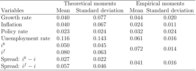
Table 2 reports theoretical moments of our Monte Carlo simulations and the
relative empirical counterparts taken from US data from 1990:Q1 to 2015:Q4.
In general, the model presents a higher volatility with respect to the data due
to the decision of linking employment to the sector of capital goods that is
to replicate satisfactorily several stylized facts especially the ones related to
[image:30.595.104.508.232.380.2]interest rates and spreads
Table 2: Theoretical and empirical moments of Monte Carlo simulations
Theoretical moments Empirical moments
Variables Mean Standard deviation Mean Standard deviation
Growth rate 0.040 0.077 0.044 0.020
Inflation 0.040 0.067 0.024 0.011
Policy rate 0.023 0.024 0.032 0.024
Unemployment rate 0.116 0.143 0.061 0.016
ik 0.050 0.045
0.072 0.014
if 0.080 0.063
Spread: ik−i 0.027 0.022
0.041 0.016
Spread: if −i 0.057 0.046
Note: empirical moments are calculated on US data, 1990:Q1-2015:Q4. Source: FRED database, see data appendix for a description of the data.
In the data the average level of theBaa bonds yield is about to the 7 % on
annual base very close to the value of 6.5% found in the model. The average
level of the policy rate in the model (2.3%) is slightly lower than the value
obtained by the data (3.2%) implying an average spread between corporate
loans and the policy rate (4.2%) very close to the empirical counterpart.
3.2
Sensitivity analysis
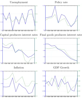
In order to check the robustness of our results, we perform a sensitivity
ex-ercise. Our parameter of interest is the coefficient related to the financial
accelerator mechanism ν. The reasons are twofolds: a) the parameter ν is
strictly related to the transmission of the monetary policy to the real
sensitivity analysis of six variables of interest over a grid of eleven
combina-tions of the parameters ν.16
The blue line reports the mean while the green
dashed line represents the standard deviation.
16
Figure 2: Sensitivity analysis
Unemployment Policy rate
Capital producers interest rates Final goods producers interest rates
Inflation GDP Growth
The solid blue line represents the mean across the Monte Carlo simulation with respect to the parameters of the financial acceleratorν. The green dotted line represents the relative standard deviation
Simulations are relatively stable across all the possible combinations of
the parameter ν, proving the robustness of our set up. The only notable
variations of the financial accelerator parameter. Their mean and standard
deviation decrease when the parameterν rises meaning a weaker effect of the
financial accelerator mechanism.17
3.3
Policy experiments
3.3.1 Monetary policy restriction
According to Taylor’s view, our simulation results show how a sudden
mone-tary policy tightness after a periods of prolonged low interest rates can have
destabilizing effects on the whole economy.
Figure 3 reports the simulated time series of twelve variables in a selected
period of time: the policy rate and the corporate loans interest rates (both
for capital producers and consumption goods producers), the unemployment
rate, the GDP growth rate, the inflation rate, the quantity of capital
recov-ered by the bank after firms’ defaults, firms’ real liquidity, the total loans
and the amount of external funds that is needed to refinance firm’s past debt,
firms’ net worth, the ratio between public debt and GDP, the production of
capital and the relative stock of inventories, the ratio between bank’s bad
debt and the total amount of loans, the wage inflation.
Central bank keeps the nominal interest rate quite low for about 20
pe-riods in response to a previous slow down of the economy that determined
an increase of the unemployment rate. The low level of the policy rate, very
close to the ZLB, successfully restore full employment and high GDP growth.
The stabilization of the economy is followed by an increase of loans provided
by banks to the real economy and a reduction of the bad debt over the total
amount of loans. Capital good producers restore the maximum production
17
capability. Firm’s net worth and the related available liquidity increase.
For several periods, unemployment rate is below the long run target of 8%
specified by the monetary authority. At periodt = 18, the central bank starts
to raise the short term interest rates in order to prevent an upturn of inflation.
The increase of the short term interest rate is quite sharp, from a value very
close to the ZLB to almost 4% in a short period of time, closely resembling the
behavior of the Federal Reserve at the end of the so called ”Greenspan put”
at the end of 2006 in the US. The financial accelerator mechanism amplifies
the external funding cost for both capital and consumption goods producers.
Loans demand is negatively affected by the higher corporate interest rates
and immediately begins to shrink.
Real variables reacts accordingly to the negative financial conditions of
the economy. The production of new capital decreases, negatively affecting
GDP growth and wages. Public debt over GDP increase due to the
contrac-tion of the GDP.
3.3.2 The aftermath of a large crisis event
After the great recession of 2008, the Federal Reserve brought the short term
interest rate very close to the ZLB and it kept fix to zero until December
2015, the beginning of the so called “Yellen call”. 18
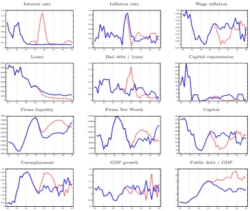
Figure 4 shows a counterfactual experiment in which the central bank
reacts accordingly to two different scenario. In the baseline one, monetary
authority returns to conduct monetary policy steering short term interest
rates following a classical Taylor rule. This allows the interest rates to be
stacked for a short period close to the ZLB and than they start to rise again
18
Figure 3: Monetary policy restriction
Policy(g), corporate(b(f),r(cp)) rates Inflation rate Wage inflation
0 0.02 0.04 0.06 0.08 0.1 0.12 0.14 0.16
0 10 20 30 40 50 60 70 -0.02 0 0.02 0.04 0.06 0.08 0.1 0.12 0.14
0 10 20 30 40 50 60 70
-0.01 0 0.01 0.02 0.03 0.04 0.05 0.06
0 10 20 30 40 50 60 70
Loans (b) Past Loans (r) Bad debt over total loans Capital repossession
0 2000 4000 6000 8000 10000 12000 14000
0 10 20 30 40 50 60 70
0 0.05 0.1 0.15 0.2 0.25 0.3
0 10 20 30 40 50 60 70 0 50 100 150 200 250
0 10 20 30 40 50 60 70
Firms liquidity Firms Net Worth Capital (r) Inventories (b)
30000 35000 40000 45000 50000 55000 60000 65000 70000 75000
0 10 20 30 40 50 60 70 60000 70000 80000 90000 100000 110000 120000 130000
0 10 20 30 40 50 60 70
0 50 100 150 200 250
0 10 20 30 40 50 60 70
Unemployment GDP Growth Public debt / GDP
0 0.05 0.1 0.15 0.2 0.25 0.3 0.35 0.4 0.45 0.5
0 10 20 30 40 50 60 70
-0.1 -0.05 0 0.05 0.1 0.15 0.2
0 10 20 30 40 50 60 70
4 5 6 7 8 9 10
0 10 20 30 40 50 60 70
as soon as the economy begins to recover.
In the alternative scenario the central bank starts to implement the
“for-ward guidance” (see Campbell et al., 2012) of the short term interest rates
committing itself to the promise that they will be kept close to the ZLB for
the necessary period of time.
The baseline scenario shows that a “double dip” recession is a major
threat when the central bank starts to rise the short term interest rate too
much and too early. Under the unlimited forward guidance scenario, the
central bank is able to stem the magnitude of the recession, at least in the
short run.
Keeping the growth rate above the level of the baseline scenario, the
central bank is able to stabilize the unemployment rate avoiding the second
recession. The accommodating monetary policy is also capable of mitigating
the credit crunch on the corporate loans market; a stabilization of the ratio
of the bad debt over total loans, due to a lower level of bad debt and a higher
level of extended loans, follows. Another significant effect is the reduction of
public debt over GDP in the ZLB scenario with respect to the baseline. The
reduction of public debt is mainly due to both higher GDP growth and the
lower interest rates paid on government bonds.19
19
Figure 4: ZLB vs no intervention by the central bank
Interest rate Inflation rate Wage inflation
Loans Bad debt / loans Capital repossession
Firms liquidity Firms Net Worth Capital
Unemployment GDP growth Public debt / GDP
The red dashed line represents the scenario in which the central bank return to the standard Taylor rule immediately after the crisis while the blue line represents the zero
4
Concluding remarks
This paper contributes to the growing literature on the post crisis behavior
of monetary authority. In order to do that we built an ABM model with a
financial accelerator mechanism like in Bernanke et al. (1999). The
simula-tions show that a scenario where the central bank is able to keep the short
term interest rates very close to the zero lower bound for an extended period
of time can help the economy to better react to large crisis events, at least
in the short run. Such intervention can potentially avoid a “double dip”
re-cession where a fragile recovery is hampered by a premature increase of the
policy rate by the central bank.
The ABM framework potentially can have several advantages over the
traditional DSGE model in several aspects. Firstly, the ABM model allows
us to fully manage heterogeneity, an essential ingredients of models with
financial intermediaries. Secondly, it allows us to simulate endogenously
large scale crises and the relative monetary policy responses.
As stated by Howitt (2012), ABM can be used by the policy makers
along-side with the traditional DSGE models allowing them evaluate the possible
policy implications from a different perspective and an alternative economic
theory.
In this context our contribution can be viewed as one of the first attempts
to evaluate unconventional monetary policies in a framework different from
the standard DSGE model.
Many potential issues are not covered in this contribution and they are
left for further research. A first class priority will be to conduct a deep
comparison between the standard financial accelerator mechanism and the
that do not burst in the financial sector but that occurred in the real side of
the economy.
5
Acknowledgment
The authors would like to thanks the participants to the 20th Workshop on
Economics with Heterogeneous Interacting Agents (WEHIA), Sophia
Antipo-lis, May 21-23, 2015 for valuable comments and suggestions. The research
leading to these results received funding from the European Union, Seventh
References
Quamrul Ashraf, Boris Gershman, and Peter Howitt. How inflation affects
macroeconomic performance: An agent-based computational investigation.
Macroeconomic Dynamics, 20(Special Issue 02):558–581, 2016.
Zakaria Babutsidze. Asymmetric (s,s) pricing: Implications for monetary
policy. Revue de l’OFCE, 124:177–204, 2012.
Ben S. Bernanke, Mark Gertler, and Simon Gilchrist. The financial
accel-erator in a quantitative business cycle framework. In J. B. Taylor and
M. Woodford, editors, Handbook of Macroeconomics, volume 1 of
Hand-book of Macroeconomics, chapter 21, pages 1341–1393. June 1999.
Michael D. Bordo and John Landon-Lane. Does Expansionary Monetary
Policy Cause Asset Price Booms; Some Historical and Empirical Evidence.
NBER Working Papers 19585, National Bureau of Economic Research, Inc,
October 2013.
Micha l Brzoza-Brzezina, Marcin Kolasa, and Krzysztof Makarski. The
anatomy of standard dsge models with financial frictions. Journal of
Eco-nomic Dynamics and Control, 37(1):32–51, 2013.
Jeffrey R. Campbell, Charles L. Evans, Jonas D.M. Fisher, and Alejandro
Justiniano. Macroeconomic Effects of Federal Reserve Forward Guidance.
Brookings Papers on Economic Activity, 44(1 (Spring):1–80, 2012.
Charles T Carlstrom and Timothy S Fuerst. Agency costs, net worth, and
business fluctuations: A computable general equilibrium analysis.
Silvano Cincotti, Marco Raberto, and Andrea Teglio. Credit money and
macroeconomic instability in the agent-based model and simulator eurace.
Economics - The Open-Access, Open-Assessment E-Journal, 4(26), 2010.
Silvano Cincotti, Marco Raberto, and Andrea Teglio. Debt deleveraging and
business cycles. an agent-based perspective.Economics - The Open-Access,
Open-Assessment E-Journal, 6(27), 2012a.
Silvano Cincotti, Marco Raberto, and Andrea Teglio. Macroprudential
poli-cies in an agent-based artificial economy. Revue de l’OFCE, 124:205–234,
2012b.
Michel Alexandre da Silva and Gilberto Tadeu Lima. Combining monetary
policy and financial regulation: an agent-based modeling approach.
Work-ing Paper, 394, 2015.
Herbert Dawid and Michael Neugart. Agent-based models for economic
pol-icy design. Eastern Economic Journal, 37(1):44–50, 2011.
Domenico Delli Gatti, Edoardo Gaffeo, and Mauro Gallegati. The apprentice
wizard: Monetary policy, complexity and learning. New Mathematics and
Natural Computation, 1(1):109–128, 2005.
Giovanni Dosi, Giorgio Fagiolo, Mauro Napoletano, and Andrea Roventini.
Income distribution, credit and fiscal policies in an agent-based
keyne-sian model. Journal of Economic Dynamics and Control, 37(8):1598–1625,
2013.
Giovanni Dosi, Giorgio Fagiolo, Mauro Napoletano, Andrea Roventini,
and Tania Treibich. Fiscal and monetary policies in complex evolving
economies. Journal of Economic Dynamics and Control, 52(C):166–189,
Giorgio Fagiolo and Andrea Roventini. Macroeconomic policy in
dsge and agent-based models. SSRN Working Paper Series,
http://ssrn.com/abstract=2011717, 2012.
Andrea Ferrero. House Price Booms, Current Account Deficits, and Low
Interest Rates. Journal of Money, Credit and Banking, 47(S1):261–293, 03
2015.
Michele Fratianni and Federico Giri. The Tale of Two Great Crises. Mo.Fi.R.
Working Papers 117, Money and Finance Research group (Mo.Fi.R.)
-Univ. Politecnica Marche - Dept. Economic and Social Sciences, December
2015.
Jean-Luc Gaffard and Mauro Napoletano. Agent-based models and economic
policy. Revue de l’OFCE, Debates and Policies, 2012.
Andrea Gerali, Stefano Neri, Luca Sessa, and Federico M. Signoretti. Credit
and banking in a dsge model of the euro area. Journal of Money, Credit
and Banking, 42(s1):107–141, 09 2010.
Simon Gilchrist and Egon Zakrajsek. Credit Spreads and Business Cycle
Fluctuations. American Economic Review, 102(4):1692–1720, June 2012.
Gottfried Haber. Monetary and fiscal policy analysis with an agent-based
macroeconomic model. Jahrbucher fur Nationalokonomie und Statistik,
228(2-3):276–295, 2008.
Peter Howitt. What have central bankers learned from modern
macroeco-nomic theory? Journal of Macroeconomics, 34(1):11–22, 2012.
Sebastian Krug, Matthias Lengnick, and Hans-Werner Wohltmann. The
impact of basel iii on financial (in)stability - an agent-based credit network
approach. Quantitative Finance, 15(12):1917–1932, 2015.
Vincenzo Quadrini. Financial frictions in macroeconomic fluctations.
Eco-nomic Quarterly, (3Q):209–254, 2011.
Luca Riccetti, Alberto Russo, and Mauro Gallegati. An agent based
decen-tralized matching macroeconomic model. Journal of Economic Interaction
and Coordination, 10(2):305–332, October 2015.
Luca Riccetti, Alberto Russo, and Mauro Gallegati. Financial regulation and
endogenous macroeconomic crises. Macroeconomic Dynamics,
forthcom-ing, 2016.
Alberto Russo, Michele Catalano, Edoardo Gaffeo, Mauro Gallegati, and
Mauro Napoletano. Industrial dynamics, fiscal policy and r&d: Evidence
from a computational experiment. Journal of Economic Behavior and
Organization, 64(3-4):426–447, 2007.
Isabelle Salle, Murat Yildizoglu, and Marc-Alexandre S´en´egas. Inflation
tar-geting in a learning economy: an abm perspective. Economic Modelling,
34(C):114–128, 2013.
John B. Taylor. Discretion versus policy rules in practice. Carnegie-Rochester
Conference Series on Public Policy, 39(1):195–214, December 1993.
John B. Taylor. Housing and Monetary Policy. NBER Working Papers
13682, National Bureau of Economic Research, Inc, December 2007.
Analysis of What Went Wrong. NBER Working Papers 14631, National
6
Data appendix
Policy rate: Effective Federal Funds Rate (FEDFUNDS), percentage,
non seasonal adjusted.
Corporate loans rates: Baa corporate bond yields (BAA) ,
percent-age, non seasonal adjusted.
Consumer price index: Consumer Price Index for All Urban
Con-sumers: All Items (CPIAUCSL), 1982-84=100, non seasonal adjusted.
Unemployment rate: Civilian Unemployment Rate (UNRATE),
per-centage, seasonal adjusted.
Gross domestic product: Gross Domestic Product (GDP), Billions