warwick.ac.uk/lib-publications
Original citation:
Patrick, Christopher E., Kumar, Santosh, Balakrishnan, Geetha, Edwards, R. S. (Rachel S.),
Lees, Martin R., Petit, Leon and Staunton, Julie B. (2018) Calculating the magnetic anisotropy
of rare-earth/transition-metal ferrimagnets. Physical Review Letters, 120 (9). 097202.
Permanent WRAP URL:
http://wrap.warwick.ac.uk/98739
Copyright and reuse:
The Warwick Research Archive Portal (WRAP) makes this work by researchers of the
University of Warwick available open access under the following conditions. Copyright ©
and all moral rights to the version of the paper presented here belong to the individual
author(s) and/or other copyright owners. To the extent reasonable and practicable the
material made available in WRAP has been checked for eligibility before being made
available.
Copies of full items can be used for personal research or study, educational, or not-for-profit
purposes without prior permission or charge. Provided that the authors, title and full
bibliographic details are credited, a hyperlink and/or URL is given for the original metadata
page and the content is not changed in any way.
Publisher statement:
© 2018 American Physical Society
Published version: https://doi.org/10.1103/PhysRevLett.120.097202
A note on versions:
The version presented here may differ from the published version or, version of record, if
you wish to cite this item you are advised to consult the publisher’s version. Please see the
‘permanent WRAP url’ above for details on accessing the published version and note that
access may require a subscription.
Christopher E. Patrick,1,∗ Santosh Kumar,1 Geetha Balakrishnan,1 Rachel
S. Edwards,1 Martin R. Lees,1 Leon Petit,2 and Julie B. Staunton1
1
Department of Physics, University of Warwick, Coventry CV4 7AL, United Kingdom 2Daresbury Laboratory, Daresbury, Warrington WA4 4AD, United Kingdom
(Dated: January 30, 2018)
Magnetocrystalline anisotropy, the microscopic origin of permanent magnetism, is often explained in terms of ferromagnets. However, the best performing permanent magnets based on rare earths and transition metals (RE-TM) are in factferrimagnets, consisting of a number of magnetic sub-lattices. Here we show how a naive calculation of the magnetocrystalline anisotropy of the classic RE-TM ferrimagnet GdCo5 gives numbers which are too large at 0 K and exhibit the wrong tem-perature dependence. We solve this problem by introducing a first-principles approach to calculate temperature-dependent magnetization vs. field (FPMvB) curves, mirroring the experiments actually used to determine the anisotropy. We pair our calculations with measurements on a recently-grown single crystal of GdCo5, and find excellent agreement. The FPMvB approach demonstrates a new level of sophistication in the use of first-principles calculations to understand RE-TM magnets.
High-performance permanent magnets, as found in generators, sensors and actuators, are characterized by a large volume magnetization and a high coercivity [1]. The coercivity — which measures the resistance to de-magnetization by external fields — is upper-bounded by the material’s magnetic anisotropy [2], which in quali-tative terms describes a preference for magnetization in particular directions. Magnetic anisotropy may be parti-tioned into two contributions: the shape anisotropy, de-termined by the macroscopic dimensions of the sample, and the magnetocrystalline anisotropy (MCA), which de-pends only on the material’s crystal structure and chem-ical composition. Horseshoe magnets provide a practchem-ical demonstration of shape anisotropy, but the MCA is less intuitive, arising from the relativistic quantum mechani-cal coupling of spin and orbital degrees of freedom [3].
Permanent magnet technology was revolutionized with the discovery of the rare-earth/transition-metal (RE-TM) magnet class, beginning with Sm-Co magnets in 1967 [4] (whose high-temperature performance is still un-matched [5]), followed by the world-leading workhorse magnets based on Nd-Fe-B [6, 7]. With the TM pro-viding the large volume magnetization, careful choice of RE yields MCA values which massively exceed the shape anisotropy contribution [8]. RE-TM magnets are now indispensable to everyday life, but their significant eco-nomic and environmental cost has inspired a global search effort aimed at replacing the critical materials re-quired in their manufacture [9].
In order to perform a targeted search for new materi-als it is necessary to fully understand the huge MCA of existing RE-TM magnets. An impressive body of theo-retical work based on crystal field theory has been built up over decades [10], where model parameters are de-termined from experiment (e.g. Ref. [11]) or electronic structure calculations [12, 13]. An alternative and in-creasingly more common approach is to use these elec-tronic structure calculations, usually based on
density-functional theory (DFT), to calculate the material’s mag-netic properties directly without recourse to the crystal field picture [14–18].
Calculating the MCA of RE-TM magnets presents a number of challenges to electronic structure theory. The interaction of localized RE-4f electrons with their itiner-ant TM counterparts is poorly described within the most widely-used first-principles methodology, the local spin-density approximation (LSDA) [12]. Indeed, the MCA is inextricably linked to orbital magnetism whose con-tribution to the exchange-correlation energy is missing in spin-only DFT [19, 20]. MCA energies are generally a few meV per formula unit, necessitating a very high degree of numerical convergence [21]. Finally, the MCA depends strongly on temperature, so a practical theory of RE-TM magnets must go beyond zero-temperature DFT and include thermal disorder [22].
Even when these significant challenges have been over-come, there is a more fundamental problem. Experi-ments access the MCA indirectly, measuring the change in magnetization of a material when an external field is applied in different directions. By contrast, calcula-tions usually access the MCA directly by evaluating the change in energy when the material is magnetized in dif-ferent directions, with no reference to an external field. These experimental and computational approaches ar-rive at the same MCA energy provided one is studying a
ferromagnet. However, the majority of RE-TM magnets (and many other technologically-important magnetic ma-terials) areferrimagnets, i.e. they are composed of sub-lattices with magnetic moments of distinct magnitudes and orientations. Crucially the application of an external field may introduce canting between these sublattices, af-fecting the measured magnetization. Thus the standard theoretical approach of ignoring the external field is hard to reconcile with real experiments on ferrimagnets.
2
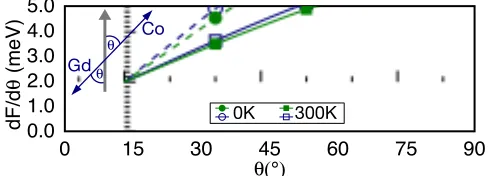
FIG. 1. Data points and fits ofdF/dθcalculated for GdCo5 (blue, empty symbols; Gd and Co moments held antiparallel) and YCo5 (green, filled symbols), at 0 and 300 K.
between electronic structure theory and practical mea-surements of the MCA. Specifically, we show how to directly simulate experiments by calculating, from first principles (FP), how the measured magnetization (M) varies as a function of field (B) applied along different directions and at different temperatures. We apply our “FPMvB” approach to the RE-TM ferro and ferrimag-nets YCo5 and GdCo5, which are isostructural to the
technologically-important SmCo5 [23] and, in the case of
GdCo5, a source of controversy in the literature [24–34].
Pairing FPMvB with new measurements of the MCA of GdCo5allows us to resolve this controversy. More
gener-ally, FPMvB enables a new level of collaboration between theory and experiment in understanding the magnetic anisotropy of ferrimagnetic materials.
The electronic structure theory behind FPMvB treats magnetic disorder at a finite temperature T within the disordered local moment (DLM) picture [35, 36]. The methodology allows the calculation of the magnetiza-tion of each sublattice i, Mi(T) = Mi(T)Mˆi, and
the torque quantity ∂F(T)/∂Mˆi, where F is an
ap-proximation to the temperature dependent free energy.
∂F(T)/∂Mˆiaccounts for the anisotropy arising from the
spin-orbit interaction, while the contribution from the classical magnetic dipole interaction is computed numer-ically [37]. Many of the technical details of the DFT-DLM calculations [35, 38–42] were described in our recent study of the magnetization of the same compounds [43]; the extensions to calculate the torques are described in Ref. [36]. The Gd-4f electrons are treated with the local self-interaction correction [42], and we have also imple-mented the orbital polarization correction [19] following Refs. [44, 45] using reported Racah parameters [46]. De-tails are given as Supplemental Material (SM) [47].
YCo5 and GdCo5 crystallize in the CaCu5
struc-ture, consisting of alternating hexagonal RCo2c/Co3g
lay-ers [23]. Y is nonmagnetic, while in GdCo5 the large
spin moment of Gd (originating mainly from its half-filled 4f shell) aligns antiferromagnetically with the Co moments. We now consider a “standard” calculation of the MCA based on a rigid rotation of the magnetiza-tion. If the Gd and Co moments are held antiparallel, GdCo5is effectively a ferromagnet with reduced moment
MCo −MGd. Then, from the hexagonal symmetry we expect the angular dependence of the free energy to fol-lowκ1sin2θ+κ2sin4θ+O(sin6θ), whereθ is the polar angle between the crystallographicc axis and the mag-netization direction. The constantsκ1, κ2 determine the
change in free energy ∆F, calculated e.g. from the force theorem [48] or the torquedF/dθ[49].
In Fig. 1 we show dF/dθ calculated for ferromagnetic YCo5 and GdCo5 at 0 and 300 K. Fitting the data to
the derivative of the textbook expression, sin 2θ(κ1 +
2κ2sin2θ), finds κ1 and κ2 to be positive (easy c axis)
withκ1an order of magnitude larger thanκ2.
Consider-ing experimentally measured anisotropy constants in the literature, for YCo5ourκ1value of 3.67 meV (all energies
are per formula unit, f.u.) at 0 K compares favorably to the values of 3.6 and 3.9 meV reported in Refs. [27] and [50]. At 300 K, our value of 2.19 meV exhibits a slightly faster decay with temperature compared to experiment (2.6 and 3.0 meV), which we attribute to our use of a classical spin hamiltonian in the DLM picture [35, 43]. However, for GdCo5 our calculated values of κ1 show
very poor agreement with experiments [25, 28]. First, at 0 K we findκ1to be larger than YCo5(4.26 meV), while
experimentally the anisotropy constant is much smaller (1.5, 2.1 meV). Second, we findκ1 decreases with
tem-perature (2.39 meV at 300 K) while experimentally the anisotropy constantincreases (2.7, 2.8 meV).
To understand these discrepancies we must ask how the anisotropy energies were actually measured. Torque magnetometry provides an accurate method of accessing the MCA [51], but is technically challenging in RE-TM magnets, which require very high fields to reach satu-ration [52]. Singular point detection [53] and ferromag-netic resonance [54] has also been used to investigate the MCA of polycrystalline and thin-film samples. However, the most commonly-used method for RE-TM magnets, employed in Refs. [25, 28], is based on the seminal 1954 work by Sucksmith and Thompson [55] on the anisotropy of hexagonal ferromagnets. This work provides a relation between the measured magnetizationMaband fieldB ap-plied in the hard plane in terms ofκ1, κ2 and the easy
axis magnetizationM0[47, 55]:
(BM0/2)/(Mab/M0)≡η=κ1+ 2κ2(Mab/M0) 2
. (1)
Further introducingm = (Mab/M0), equation 1 shows that a plot ofη against m2 should yield a straight line withκ1 as the intercept. Even though this “Sucksmith-Thompson method” was derived for ferromagnets, the technical procedure of plottingηagainstm2can be
per-formed also for ferrimagnets like GdCo5 [25, 28]. In
this case, the quantity extracted from the intercept is an effective anisotropy constant Keff so, unlike YCo5, the
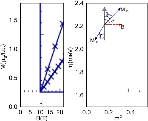
FIG. 2. Magnetization of GdCo5 vs. applied magnetic field shown on a standard plot (left panel) or after the Sucksmith-Thompson analysis (eq. 1, right panel). Crosses/circles are calculated with methods (i)/(ii) discussed in the text, and the area between them shaded as a guide to the eye. Note the two methods are effectively indistinguishable in the left panel. The dashed/solid lines are calculated from the model free energiesF1 andF2. The right panel also shows the ge-ometry of the magnetization and field with respect to the crystallographicc-axis (thick gray arrow).
the reduced value ofKeff with respect toκ1of YCo5 is a
fingerprint of canting between the Gd and Co sublattices. Making contact with previous experiments thus re-quires we obtain Keff. To this end we have developed a
scheme of calculating first-principles hard-plane magne-tization vs. field (FPMvB) curves, on which we perform the Sucksmith-Thompson analysis to directly mirror the experiments. The central concept of FPMvB is that at equilibrium, the torques from the exchange, spin-orbit and dipole interactions must balance those arising from the external field. Then,
B= ∂F(T)
∂θi
1
Micosθi+Pjsinθj ∂Mj
∂θi
. (2)
The magnetization at a givenB, T is determined by the angle set {θGd, θCo1, θCo2, ...} which satisfies equation 2
for every magnetic sublattice. The spin-orbit interaction breaks the symmetry of the Co3g atoms such that
al-together there are four independent angles to vary for GdCo5. The second term in the denominator of
equa-tion 2 reflects that the magnetic moments themselves might depend onθi(magnetization anisotropy). We have
tested (i) neglecting this contribution and (ii) modeling the dependence as Mi(θi) = M0i(1−pisin2θi), where
M0i andpi are parameterized from our calculations.
Figure 2 shows FPMvB curves of GdCo5 calculated
using equation 2 with methods (i) and (ii), (crosses and
circles) which yield virtually identical values ofKeff. The
M vs.Bcurves in the left panel resemble those of a ferro-magnet where, as the temperature increases, it becomes easier to rotate the moments away from the easy axis so that a given B field induces a larger magnetization. However, plottingη againstm2in the right panel tells a
more interesting story. The effective anisotropy constant
Keff (y-axis intercept) at 0 K is 1.53 meV, much smaller
thanκ1 of YCo5. FurthermoreKeff increases with
tem-perature, to 1.74 meV at 300 K. Therefore, in contrast to the standard calculations of Fig. 1, the FPMvB approach reproduces the experimental behavior of Refs. [25, 28].
Our FPMvB calculations provide a microscopic insight into the magnetization process. For instance at 0 K and 9 T, we calculate that the cobalt moments rotate away from the easy axis by 6.1◦. By contrast the Gd moments have rotated by only 3.9◦, i.e. the ideal 180◦ Gd-Co alignment has reduced by 2.2◦ (the geometry is shown in Fig. 2). We also find canting between the dif-ferent Co sublattices, but not by more than 0.1◦ at both
0 and 300 K (the calculated angles as a function of field are shown in the SM [47]). This Co-Co canting is small thanks to the Co-Co ferromagnetic exchange interaction, which remains strong over a wide temperature range [43]. The temperature dependence of Keff can be traced to the fact that the easy axis magnetizationM0 of GdCo5
initially increases with temperature [43]. Even if Mab
increases with temperature at a given field, a faster in-crease in M0 can lead to an overall hardening in Keff
(equation 1).
We assign the canting in GdCo5to a delicate
competi-tion between the exchange interaccompeti-tion favoring antiparal-lel Co/Gd moments, uniaxial anisotropy favoringc-axis (anti)alignment, and the external field trying to rotate all moments into the hard plane. We can quantify these in-teractions by looking for a model parameterization of the free energyF. Crucially we can train the model with an arbitrarily large set of first-principles calculations explor-ing sublattice orientations not accessible experimentally, and test its performance against the torque calculations of equation 2. Neglecting the 0.1◦ canting within the cobalt sublattices gives two free angles,θGdandθCo. In-cluding Gd-Co exchangeA, uniaxial Co anisotropyK1,Co
and a dipolar contributionS(θGd, θCo) [30, 47] leads nat-urally to a two-sublattice model [29],
F1(θGd, θCo) =−Acos(θGd−θCo) +K1,Cosin2θCo
+S(θGd, θCo). (3)
The training calculations showed additional angular de-pendences not captured byF1, so we also investigated:
F2(θGd, θCo) =F1(θGd, θCo) +K2,Cosin4θCo
+K1,Gdsin2θGd. (4)
4
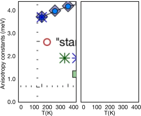
FIG. 3. Anisotropy constantsKeff vs. temperature of YCo5 (green) and GdCo5 (blue). The left panel shows calculations using equation 2 at 0 and 300 K (stars), or using parameter-ized model expressions F1 (diamonds) and F2 (circles), and from Ref. [56] (YCo5, squares). For GdCo5 we also show in redκ1 extracted from “standard” calculations where the Gd and Co moments were held rigidly antiparallel (cf. Fig. 1). The experimental data in the right panel was measured by us for GdCo5 (crosses, with shaded background) or taken from Refs. [25], [28] and [57] (squares, dashed lines, circles) and Refs [27] and [50] (green diamonds and dashed lines, YCo5).
The dashed (solid) lines in Fig. 2 are the calculatedM
vs.B curves obtained by minimizingF1(2)−P
iMi·B.
The second term includes magnetization anisotropy on the cobalt moments [47, 56]. On the scale of the left panel both F1 and F2 give excellent fits to the torque
calculations, especially up to moderate fields. The plot of η againstm2 reveals some differences withF
2 giving
a marginally improved description of the data, but F1
already captures the most important physics.
We also applied the FPMvB approach to YCo5, using
equation 2 and the model forF introduced in Ref. [56]. Then, parameterizing the models [47] over the tempera-ture range 0–400 K, calculating M vs.B curves and ex-tractingKeff using the Sucksmith-Thompson plots gives
the results shown in the left panel of Fig. 3. We also show κ1 of GdCo5 to emphasize the difference between
FPMvB calculations and the “standard” ones of Fig. 1. Comparing Keff to previously-published experimental measurements on GdCo5 raises some issues. First, the
three studies in the literature report anisotropy constants which differ by as much as 1 meV [25, 28, 57]. Indeed there was controversy over whether the observed results were evidence of an anisotropic exchange interaction be-tween Gd and Co [30, 31] or an artefact of poor sam-ple stoichiometry [32, 33]. Furthermore the only study performed above room temperature [25] reports without comment some peculiar behavior where Keff of GdCo5
exceeds that of YCo5 at high temperature [27], despite
conventional wisdom that the half-filled 4f shell of Gd does not contribute to the anisotropy.
Our calculations do in fact show an excess in the rigid-moment anisotropy of GdCo5 of 16% at 0 K (Fig. 1)
compared to YCo5. The authors of Refs. [28, 30]
fit-ted their experimental data with a much larger excess of 50%, while the high-field study of Ref. [32] found (11±
15)%, with the authors of that work attributing the dif-ference to an improved sample stoichiometry [33]. Our calculated excess at 0 K is formed from two major contri-butions: the dipole interaction energy, which accounts for 0.31 meV/f.u., andK1,Gd (equation 4) which we found
to be 24% the size ofK1,Co. The nonzero value ofK1,Gd
is due to the 5delectrons, whose presence is evident from the Gd magnetization (7.47µB at 0 K). We did not find a
significant contribution from anisotropic exchange, which we tested in two ways: first by attempting to fit a term
A(1−p0sin2θCo) cos(θGd−θCo) to our training set of
calculations, and also by computing Curie temperatures with the (rigidly antiparallel) magnetization directed ei-ther along thec or a axes. We found the magnitude of the anisotropy (p0) to be smaller than 0.5% and negative at 0 K, and to decrease in magnitude as the temperature is raised. Consistently the Curie temperature was found to be only 1 K higher foraaxis alignment, which we do not consider significant.
However, our calculations do not predict theKeff value
of GdCo5to exceed YCo5. Indeed, in Fig. 3κ1of GdCo5
approaches that of YCo5 at high temperatures, which
is significant because κ1 provides an upper bound for Keff [31]. To resolve this final puzzle we performed our own measurements of Keff on the single crystal whose growth we reported recently [43]. Hard and easy axis magnetization curves up to 7 T were measured in a Quan-tum Design superconducting quanQuan-tum interference de-vice (SQUID) magnetometer, and the anisotropy con-stants extracted from Sucksmith-Thompson plots [47]. The right panel of Fig. 3 shows our newly measured data as crosses. Previously reported measurements are shown in faint blue/green for GdCo5[25, 28, 57]/YCo5[27, 50].
Up to 200 K, there is close agreement between the experiments of Ref. [25], our own experiments, and the FPMvB calculations. Above this temperature our new experiments show the expected drop in Keff, while the previously reported data show a continued rise [25]. We repeated our measurements using different protocols and found a reasonably large variation in the extracted
Keff [47]. Even taking this variation into account as the shaded area in Fig. 3, the drop is still observed.
We therefore do not believe the high temperature be-havior reported in Ref. [25] has an intrinsic origin. Possi-ble extrinsic factors include the method of sample prepa-ration, degradation of the RCo5 phase at elevated
curves in Fig. 2 show curvature at higher temperature, making it more difficult to find the intercept.
In conclusion, we have introduced the FPMvB ap-proach to interpret experiments measuring anisotropy of ferrimagnets, particularly RE-TM permanent magnets. We presented the method in the context of our CPA formalism, but any electronic structure theory capable of calculating magnetic couplings relativistically [59–63] should be able to produce FPMvB curves, at least at zero temperature. However standard calculations which neglect the external field should be used with care when comparing to experiments on ferrimagnets. Similarly, the prototype GdCo5 serves as a reminder that a
sim-ple view of the anisotropy energy does not fully describe the magnetization processes in ferrimagnets, which might have implications in understanding e.g. magnetization reversal in nano-magnetic assemblies [64]. Overall our work demonstrates the benefit of interconnected compu-tational and experimental research in this key area.
The present work forms part of the PRETAMAG project, funded by the UK Engineering and Phys-ical Sciences Research Council (EPSRC), Grant no. EP/M028941/1. Crystal growth work at Warwick is also supported by EPSRC Grant no. EP/M028771/1. Work at Daresbury Laboratory was supported by an EPSRC service level agreement with the Scientific Computing De-partment of STFC. We thank E. Mendive-Tapia for use-ful discussions and A. Vasylenko for continued assistance in translating references.
∗
c.patrick.1@warwick.ac.uk
[1] S. Chikazumi,Physics of Ferromagnetism, 2nd ed. (Ox-ford University Press, 1997).
[2] H. Kronm¨uller, Phys. Stat. Sol. b144, 385 (1987). [3] P. Strange,Relativistic Quantum Mechanics(Cambridge
University Press, 1998).
[4] K. Strnat, G. Hoffer, J. Olson, W. Ostertag, and J. J. Becker, J. Appl. Phys. 38, 1001 (1967).
[5] O. Gutfleisch, M. A. Willard, E. Br¨uck, C. H. Chen, S. G. Sankar, and J. P. Liu, Adv. Mater.23, 821 (2011). [6] M. Sagawa, S. Fujimura, N. Togawa, H. Yamamoto, and
Y. Matsuura, J. Appl. Phys.55, 2083 (1984).
[7] J. J. Croat, J. F. Herbst, R. W. Lee, and F. E. Pinkerton, J. Appl. Phys.55, 2078 (1984).
[8] J. M. D. Coey, IEEE Trans. Magn.47, 4671 (2011). [9] R. Skomski, P. Manchanda, P. Kumar, B. Balamurugan,
A. Kashyap, and D. J. Sellmyer, IEEE Trans. Magn.49, 3215 (2013).
[10] M. D. Kuz’min and A. M. Tishin, inHandbook of Mag-netic Materials, Vol. 17, edited by K. H. J. Buschow (El-sevier B.V., 2008) Chap. 3, p. 149.
[11] Z. Tie-song, J. Han-min, G. Guang-hua, H. Xiu-feng, and C. Hong, Phys. Rev. B43, 8593 (1991).
[12] M. Richter, J. Phys. D: Appl. Phys.31, 1017 (1998). [13] P. Delange, S. Biermann, T. Miyake, and L. Pourovskii,
Phys. Rev. B96, 155132 (2017).
[14] L. Steinbeck, M. Richter, and H. Eschrig, J. Magn. Magn. Mater.226–230, Part 1, 1011 (2001).
[15] P. Larson, I. I. Mazin, and D. A. Papaconstantopoulos, Phys. Rev. B69, 134408 (2004).
[16] H. Pang, L. Qiao, and F. S. Li, Phys. Status Solidi B 246, 1345 (2009).
[17] M. Matsumoto, R. Banerjee, and J. B. Staunton, Phys. Rev. B90, 054421 (2014).
[18] A. Landa, P. S¨oderlind, D. Parker, D. ˚Aberg, V. Lordi, A. Perron, P. E. A. Turchi, R. K. Chouhan, D. Paudyal, and T. A. Lograsso, “Thermodynamics of the SmCo5 compound doped with Fe and Ni: an ab initio study,” (2017), arXiv:1707.09447.
[19] O. Eriksson, B. Johansson, R. C. Albers, A. M. Boring, and M. S. S. Brooks, Phys. Rev. B42, 2707 (1990). [20] H. Eschrig, M. Sargolzaei, K. Koepernik, and M. Richter,
Europhys. Lett.72, 611 (2005).
[21] G. H. O. Daalderop, P. J. Kelly, and M. F. H. Schuur-mans, Phys. Rev. B53, 14415 (1996).
[22] J. B. Staunton, S. Ostanin, S. S. A. Razee, B. L. Gyorffy, L. Szunyogh, B. Ginatempo, and E. Bruno, Phys. Rev. Lett.93, 257204 (2004).
[23] K. Kumar, J. Appl. Phys.63, R13 (1988).
[24] K. Buschow, A. van Diepen, and H. de Wijn, Solid State Commun.15, 903 (1974).
[25] A. Ermolenko, IEEE Trans. Mag.12, 992 (1976). [26] S. Rinaldi and L. Pareti, J. Appl. Phys.50, 7719 (1979). [27] A. S. Yermolenko, Fiz. Metal. Metalloved.50, 741 (1980). [28] R. Ballou, J. D´eportes, B. Gorges, R. Lemaire, and
J. Ousset, J. Magn. Magn. Mater.54, 465 (1986). [29] R. Radwa´nski, Physica B+C142, 57 (1986).
[30] R. Ballou, J. D´eportes, and J. Lemaire, J. Magn. Magn. Mater.70, 306 (1987).
[31] P. Gerard and R. Ballou, J. Magn. Magn. Mater.104, 1463 (1992).
[32] R. Radwa´nski, J. Franse, P. Quang, and F. Kayzel, J. Magn. Magn. Mater.104, 1321 (1992).
[33] J. J. M. Franse and R. J. Radwa´nski, in Handbook of Magnetic Materials, Vol. 7, edited by K. H. J. Buschow (Elsevier North-Holland, New York, 1993) Chap. 5, p. 307.
[34] T. Zhao, H. Jin, R. Gr¨ossinger, X. Kou, and H. R. Kirch-mayr, J. Appl. Phys.70, 6134 (1991).
[35] B. L. Gy¨orffy, A. J. Pindor, J. Staunton, G. M. Stocks, and H. Winter, J. Phys. F: Met. Phys.15, 1337 (1985). [36] J. B. Staunton, L. Szunyogh, A. Buruzs, B. L. Gyorffy,
S. Ostanin, and L. Udvardi, Phys. Rev. B 74, 144411 (2006).
[37] We performed a sum over dipoles [1] using the calculated Mi(T) out to a radius of 20 nm.
[38] E. Bruno and B. Ginatempo, Phys. Rev. B55, 12946 (1997).
[39] P. Strange, J. Staunton, and B. L. Gyorffy, J. Phys. C: Solid State Phys.17, 3355 (1984).
[40] M. D¨ane, M. L¨uders, A. Ernst, D. K¨odderitzsch, W. M. Temmerman, Z. Szotek, and W. Hergert, J. Phys.: Con-dens. Matter21, 045604 (2009).
[41] S. H. Vosko, L. Wilk, and M. Nusair, Can. J. Phys.58, 1200 (1980).
[42] M. L¨uders, A. Ernst, M. D¨ane, Z. Szotek, A. Svane, D. K¨odderitzsch, W. Hergert, B. L. Gy¨orffy, and W. M. Temmerman, Phys. Rev. B71, 205109 (2005).
6
Staunton, Phys. Rev. Materials1, 024411 (2017). [44] H. Ebert and M. Battocletti, Solid State Commun. 98,
785 (1996).
[45] H. Ebert, “Fully relativistic band structure calculations for magnetic solids - formalism and application,” in Elec-tronic Structure and Physical Properies of Solids: The Uses of the LMTO Method Lectures of a Workshop Held at Mont Saint Odile, France, October 2–5,1998, edited by H. Dreyss´e (Springer Berlin Heidelberg, Berlin, Hei-delberg, 2000) pp. 191–246.
[46] L. Steinbeck, M. Richter, and H. Eschrig, Phys. Rev. B 63, 184431 (2001).
[47] See Supplemental Material at [URL] for further experi-mental and computational details, description of the or-bital polarization correction, discussion of magnetization anisotropy, the parameters used to simulateMvBcurves and the angle sets which satisfy equation 2.
[48] G. H. O. Daalderop, P. J. Kelly, and M. F. H. Schuur-mans, Phys. Rev. B41, 11919 (1990).
[49] X. Wang, R. Wu, D.-s. Wang, and A. J. Freeman, Phys. Rev. B54, 61 (1996).
[50] J. M. Alameda, D. Givord, R. Lemaire, and Q. Lu, J. Appl. Phys.52, 2079 (1981).
[51] H. Klein, A. Menth, and R. Perkins, Physica B+C80, 153 (1975).
[52] K. H. J. Buschow and F. R. de Boer,Physics of
Mag-netism and Magnetic Materials (Springer, Boston, MA, 2003).
[53] A. Paoluzi, L. Pareti, M. Solzi, and F. Albertini, J. Magn. Magn. Mater.132, 185 (1994).
[54] Y. Wang, Y. Zhao, S. Wang, M. Lu, H. Zhai, Y. Zhai, K. Shono, and X. Yu, J. Appl. Phys.93, 7789 (2003). [55] W. Sucksmith and J. E. Thompson, Proc. Royal Soc. A
225, 362 (1954).
[56] J. Alameda, J. D´eportes, D. Givord, R. Lemaire, and Q. Lu, J. Magn. Magn. Mater.15, 1257 (1980). [57] T. Katayama, M. Ohkoshi, Y. Koizumi, T. Shibata, and
T. Tsushima, Appl. Phys. Lett.28, 635 (1976).
[58] F. Den Broeder and K. Buschow, J. Less-Common Metals 29, 65 (1972).
[59] L. Udvardi, L. Szunyogh, K. Palot´as, and P. Weinberger, Phys. Rev. B68, 104436 (2003).
[60] H. Ebert and S. Mankovsky, Phys. Rev. B 79, 045209 (2009).
[61] J. Hu and R. Wu, Phys. Rev. Lett.110, 097202 (2013). [62] S. Ayaz Khan, P. Blaha, H. Ebert, J. Min´ar, and O. ˇSipr,
Phys. Rev. B94, 144436 (2016).
[63] M. Hoffmann, B. Zimmermann, G. P. M¨uller, D. Sch¨urhoff, N. S. Kiselev, C. Melcher, and S. Bl¨ugel, Nat. Commun.8, 308 (2017).