warwick.ac.uk/lib-publications
Original citation:
Duong, Manh Hong, Lamacz, Agnes, Peletier, Mark A. and Sharma, Upanshu. (2017)
Variational approach to coarse-graining of generalized gradient flows. Calculus of Variations
and Partial Differential Equations, 56 . 100 .
Permanent WRAP URL:
http://wrap.warwick.ac.uk/89647
Copyright and reuse:
The Warwick Research Archive Portal (WRAP) makes this work of researchers of the
University of Warwick available open access under the following conditions.
This article is made available under the Creative Commons Attribution 4.0 International
license (CC BY 4.0) and may be reused according to the conditions of the license. For more
details see: http://creativecommons.org/licenses/by/4.0/
A note on versions:
The version presented in WRAP is the published version, or, version of record, and may be
cited as it appears here.
Variational approach to coarse-graining of generalized
gradient flows
Manh Hong Duong1 ·Agnes Lamacz2 · Mark A. Peletier3 ·Upanshu Sharma4
Received: 12 July 2015 / Accepted: 4 May 2017 / Published online: 28 June 2017 © The Author(s) 2017. This article is an open access publication
Abstract In this paper we present a variational technique that handles coarse-graining and passing to a limit in a unified manner. The technique is based on a duality structure, which is present in many gradient flows and other variational evolutions, and which often arises from a large-deviations principle. It has three main features: (a) a natural interaction between the duality structure and the coarse-graining, (b) application to systems with non-dissipative effects, and (c) application to coarse-graining of approximate solutions which solve the equation only to some error. As examples, we use this technique to solve three limit problems, the overdamped limit of the Vlasov–Fokker–Planck equation and the small-noise limit of randomly perturbed Hamiltonian systems with one and with many degrees of freedom.
Mathematics Subject Classification 35K67·35B25·49S99·49J45·35K10·35K20· 60F10·70F40·70G75·37L05·35Q99·60J60
Contents
1 Introduction . . . 2
1.1 Variational approach—an outline . . . 3
1.2 Origin of the functionalIε: large deviations of a stochastic particle system . . . 5
Communicated by L. Ambrosio.
B
Upanshu Sharma [email protected]1 Mathematics Institute, University of Warwick, Coventry, United Kingdom 2 Fakultät für Mathematik, Dortmund, Germany
3 Department of Mathematics and Computer Sciences and Institute for Complex Molecular Systems,
Technische Universiteit Eindhoven, Eindhoven, The Netherlands
1.3 Concrete problems . . . 7
1.3.1 Overdamped limit of the Vlasov–Fokker–Planck equation . . . 7
1.3.2 Small-noise limit of a randomly perturbed Hamiltonian system with one degree of freedom 7 1.3.3 Small-noise limit of a randomly perturbed Hamiltonian system withddegrees of freedom 9 1.4 Comparison with other work . . . 9
1.5 Outline of the article . . . 10
1.6 Summary of notation . . . 10
2 Overdamped limit of the VFP equation . . . 11
2.1 Setup of the system . . . 11
2.2 A priori bounds . . . 12
2.3 Coarse-graining and compactness. . . 15
2.4 Local equilibrium . . . 17
2.5 Liminf inequality . . . 17
2.6 Discussion. . . 20
3 Diffusion on a graph in one dimension . . . 20
3.1 Construction of the graph. . . 21
3.2 Adding noise: diffusion on the graph . . . 22
3.3 Compactness . . . 22
3.4 Local equilibrium . . . 24
3.5 Continuity ofρandρˆ . . . 25
3.6 Liminf inequality . . . 26
3.7 Study of the limit problem . . . 28
3.8 Conclusion and discussion . . . 32
4 Diffusion on a graph,d>1 . . . 32
5 Conclusion and discussion. . . 34
A Proof of Lemma 2.1 . . . 36
B Proof of Theorem 2.3. . . 38
C Properties of the auxiliary PDE. . . 45
C.1 Well-posedness . . . 45
C.2 Bounds and regularity properties . . . 54
C.2.1 Comparison principle and growth at infinity . . . 54
C.2.2 Regularity. . . 57
D Proof of Theorem 3.1. . . 60
References. . . 62
1 Introduction
Coarse-graining is the procedure of approximating a system by a simpler or lower-dimensional one, often in some limiting regime. It arises naturally in various fields such as thermodynamics, quantum mechanics, and molecular dynamics, just to name a few. Typi-cally coarse-graining requires a separation of temporal and/or spatial scales, i.e. the presence of fast and slow variables. As the ratio of ‘fast’ to ‘slow’ increases, some form of averaging or homogenization should allow one to remove the fast scales, and obtain a limiting system that focuses on the slow ones.
Coarse-graining limits are by naturesingular limits, since information is lost in the coarse-graining procedure; therefore rigorous proofs of such limits are always non-trivial. Although the literature abounds with cases that have been treated successfully, and some fields can even be called well-developed—singular limits in ODEs and homogenization theory, to name just two—many more cases seem out of reach, such as coarse-graining in materials [25], climate prediction [66], and complex systems [33,59].
two-scale convergence [5].Variational-evolution structure, such as in the case of gradient flows and variational rate-independent systems, also facilitates limits [28,51,53,54,67,70,
71].
In this paper we introduce and study such a structure, which arises from the theory oflarge deviationsfor stochastic processes. In recent years we have discovered that many gradient flows, and also many ‘generalized’ gradient systems, can be matched one-to-one to the large-deviation characterization of some stochastic process [2,3,24,26,27,52]. The large-deviation rate functional, in this connection, can be seen todefinethe generalized gradient system. This connection has many philosophical and practical implications, which are discussed in the references above.
We show how in such systems, described by a rate functional, ‘passing to a limit’ is facilitated by the duality structure that a rate function inherits from the large-deviation context, in a way that meshes particularly well with coarse-graining.
1.1 Variational approach—an outline
The systems that we consider in this paper are evolution equations in a space of measures. Typ-ical examples are the forward Kolmogorov equations associated with stochastic processes, but also various nonlinear equations, as in one of the examples below.
Consider the family of evolution equations
∂tρε=Nερε, ρε|t=0=ρε0,
(1)
whereNε is a linear or nonlinear operator. The unknown ρε is a time-dependent Borel measure on a state spaceX, i.e.ρε: [0,T] →M(X). In the systems of this paper, (1) has a variational formulation characterized by a functionalIεsuch that
Iε≥0 and ρεsolves (1) ⇐⇒ Iε(ρε)=0. (2)
This variational formulation is closely related to the Brezis–Ekeland–Nayroles variational principle [10,41,57,71] and the integrated energy-dissipation identity for gradient flows [4]; see Sect.5.
Our interest in this paper is the limitε → 0, and we wish to study the behaviour of the system in this limit. If we postpone the aspect of coarse-graining for the moment, this corresponds to studying the limit ofρεasε→0. Sinceρεis characterized byIε, establishing the limiting behaviour consists of answering two questions:
1. CompactnessDo solutions ofIε(ρε)=0 have useful compactness properties, allowing one to extract a subsequence that converges in a suitable topology, sayς?
2. Liminf inequalityIs there a limit functionalI ≥0 such that
ρε ς−→ρ ⇒ lim inf ε→0 I
ε(ρε)≥I(ρ)? (3)
And if so, does one have
I(ρ)=0 ⇐⇒ ρsolves∂tρ=Nρ,
for some operatorN?
A special aspect of the method of the present paper is that it also applies toapproximate
cases whenC =0. The main message of our approach is that all the results then follow from this uniform bound and assumptions on well-prepared initial data.
The compactness question will be answered by the first crucial property of the functionals
Iε, which is that they provide ana prioribound of the type
Sε(ρtε)+
t
0
Rε(ρsε)ds≤Sε(ρ0ε)+Iε(ρε), (4)
whereρtεdenotes the time slice at timetandSεandRεare functionals. In the examples of this paperSεis a free energy andRεa relative Fisher Information, but the structure is more general. This inequality is reminiscent of the energy-dissipation inequality in the gradient-flow setting. The uniform bound, by assumption, of the right-hand side of (4) implies that each term in the left-hand side of (4), i.e., the free energy at any timet >0 and the integral of the Fisher information, is also bounded. This will be used to apply the Arzelà–Ascoli theorem to obtain certain compactness and ‘local-equilibrium’ properties. All this discussion will be made clear in each example in this paper.
The second crucial property of the functionalsIεis that they satisfy a duality relation of the type
Iε(ρ)=sup f
Jε(ρ, f), (5)
where the supremum is taken over a class of smooth functions f. It is well known how such duality structures give rise to good convergence properties such as (3), but the focus in this paper is on how this duality structure combines well with coarse-graining.
In this paper we definecoarse-grainingto be a shift to a reduced, lower dimensional description via a coarse-graining mapξ:X →Ywhich identifies relevant information and is typically highly non-injective. Note thatξ may depend onε. A typical example of such a coarse-graining map is a ‘reaction coordinate’ in molecular dynamics. The coarse-grained equivalent ofρε : [0,T] →M(X)is the push-forwardρˆε :=ξ#ρε : [0,T] →M(Y). If
ρεis the law of a stochastic processXε, thenξ
#ρεis the law of the processξ(Xε).
There might be several reasons to be interested inξ#ρεrather thanρεitself. The
push-forwardξ#ρεobeys a dynamics with fewer degrees of freedom, sinceξis non-injective; this
might allow for more efficient computation. Our first example (see Sect.1.3), the overdamped limit in the Vlasov–Fokker–Planck equation, is an example of this. As a second reason, by removing certain degrees of freedom, some specific behaviour ofρεmight become clearer; this is the case with our second and third examples (Sect.1.3), where the effect ofξis to remove a rapid oscillation, leaving behind a slower diffusive movement. Whatever the reason, in this paper we assume that someξis given, and that we wish to study the limit ofξ#ρεasε→0.
The core of the arguments of this paper, that leads to the characterization of the equation satisfied by the limit ofξ#ρε, is captured by the following formal calculation:
Iε(ρε)=sup f
Jε(ρε,f)
f=g◦ξ ≥ sup
g J
ε(ρε,g◦ξ)
⏐⏐ ε→0
sup g J(ρ,
g◦ξ)
(∗) =:sup
g ˆ
Let us go through the lines one by one. The first line is the duality characterization (5) of
Iε. The inequality in the second line is due to the reduction to a subset of special functions
f, namely those of the form f =g◦ξ. This is in fact an implementation of coarse-graining: in the supremum we decide to limit ourselves to observables of the formg◦ξwhich only have access to the information provided byξ. After this reduction we pass to the limit and show thatJε(ρε,g◦ξ)converges to someJ(ρ,g◦ξ)—at least for appropriately chosen coarse-graining maps.
In the final step(∗)one requires that the loss-of-information in passing fromρtoρˆis consistent with the loss-of-resolution in considering only functions f = g◦ξ. This step requires a proof oflocal equilibrium, which describes how the behaviour ofρthat isnot
represented explicitly by the push-forward ρˆ, can nonetheless be deduced fromρˆ. This local-equilibrium property is at the core of various coarse-graining methods and is typically determined case by case.
We finally define Iˆby duality in terms of Jˆas in(∗∗). In asuccessfulapplication of this method, the resulting functionalIˆat the end has ‘good’ propertiesdespitethe loss-of-accuracy introduced by the restriction to functions of the formg◦ξ, and this fact acts as a test of success. Such good properties should include, for instance, the property thatIˆ=0 has a unique solution in an appropriate sense.
Now let us explain the origin of the functionalsIε.
1.2 Origin of the functionalIε: large deviations of a stochastic particle system
The abstract methodology that we described above arises naturally in the context oflarge deviations, and we now describe this in the context of the three examples that we discuss in the next section. All three originate from (slight modifications of) one stochastic process, that models a collection of interacting particles with inertia in the physical spaceRd:
d Qni(t)= P
n i (t)
m dt, (6a)
d Pin(t)= −∇VQni(t)dt−1 n
n
j=1
∇ψQnj(t)−Qni(t) dt− γ mP
n i (t)dt+
2γ θd Wi(t).
(6b)
HereQni ∈RdandPin∈Rd are the position and momentum of particlesi=1, . . . ,nwith massm. Equation (6a) is the usual relation betweenQ˙ni andPin, and (6b) is a force balance which describes the forces acting on the particle. For this system, corresponding to the first example below, these forces are (a) a force arising from a fixed potentialV, (b) an interaction force deriving from a potentialψ, (c) a friction force, and (d) a stochastic force characterized by independentd-dimensional Wiener measuresWi. Throughout this paper we collectQni andPininto a single variableXni =(Qni,Pin).
We now consider the many-particle limitn→ ∞in (6). It is a well-known fact that the empirical measure
ρn(t)= 1
n
n
i=1
δXni(t) (7)
converges almost surely to the unique solution of theVlasov–Fokker–Planck (VFP) equa-tion[60]
∂tρ=(Lρ)∗ρ, (Lμ)∗ρ:=−divq
ρp
m +divpρ
∇qV+∇qψ∗μ+γ
p
m +γ θ pρ,
(8)
= −divρJ∇(H+ψ∗μ)+γdivpρ
p
m +γ θpρ, (9)
with an initial datum that derives from the initial distribution ofXin. The spatial domain here isR2d with coordinates(q,p) ∈Rd ×Rd, and subscripts such as in∇
q andp indicate that differential operators act only on corresponding variables. The convolution is defined by(ψ∗ρ)(q)=R2dψ(q−q)ρ(q,p)dqd p. In the second line above we use a slightly shorter way of writingLμ∗, by introducing the HamiltonianH(q,p)=p2/2m+V(q)and the canonical symplectic matrixJ = −0I0I. This way of writing also highlights that the system is a combination of conservative effects, described byJ,H, andψ, and dissipative effects, which are parametrized byγ. The primal formLμof the operator(Lμ)∗is
Lμf = J∇(H+ψ∗μ)· ∇f −γ p
m · ∇pf +γ θpf.
The almost-sure convergence ofρnto the solutionρof the (deterministic) VFP equation is the starting point for alarge-deviationresult. In particular it has been shown that the sequence (ρn)has alarge-deviation property[9,22,26] which characterizes the probability of finding the empirical measure far from the limitρ, written informally as
Prob(ρn≈ρ)∼exp
−n 2I(ρ) ,
in terms of arate functional I :C([0,T];P(R2d))→R. If we assume that the initial data
Xinare chosen to be deterministic, and such that the initial empirical measureρn(0)converges narrowly to someρ0, thenI has the form [26]
I(ρ):= sup f∈Cb1,2(R×R2d)
R2d
fTdρT −
R2d
f0dρ0−
T
0
R2d
∂tf +Lρt f
dρtdt
−1 2
T
0
R2d
(f,f)dρtdt, (10)
providedρt|t=0 =ρ0, whereis the carré-du-champ operator (e.g. [11, Sect. 1.4.2])
(f,g):= 1
2
Lμ(f g)− fLμg−gLμf=γ θ∇pf∇pg.
If the initial measureρt|t=0 is not equal to the limitρ0 of the stochastic initial empirical
measures, thenI(ρ)= ∞.
(which is unique, given initial dataρ0[35]). ThereforeIis of the form that we discussed in
Sect.1.1:I≥0, andI(ρ)=0 iffρsolves (8), which is a realization of (1).
1.3 Concrete problems
We now apply the coarse-graining method of Sect.1.1to three limits: theoverdampedlimit γ → ∞, and twosmall-noiselimitsθ →0. In each of these three limits, the VFP Eq. (8) is the starting point, and we prove convergence to a limiting system using appropriate coarse-graining maps. Note that the convergence is therefore from one deterministic equation to another one; but the method makes use of the large-deviation structure that the VFP equation has inherited from its stochastic origin.
1.3.1 Overdamped limit of the Vlasov–Fokker–Planck equation
The first limit that we consider is the limit of large friction,γ → ∞, in the Vlasov–Fokker– Planck equation (8), settingθ =1 for convenience. To motivate what follows, we divide (8) throughout byγ and formally letγ → ∞to find
divpρ
p
m +pρ=0,
which suggests that in the limitγ → ∞,ρshould be Maxwellian inp, i.e.
ρt(dq,d p)=Z−1exp
−p2 2m
d pσt(dq), (11)
whereZ = (2mπ)d/2 is the normalization constant for the Maxwellian distribution. The main result in Sect.2shows that after an appropriate time rescaling, in the limitγ → ∞, the remaining unknownσ∈C([0,T];P(Rd))solves the Vlasov–Fokker–Planck equation
∂tσ =div(σ∇V(q))+div(σ (∇ψ∗σ ))+σ. (12)
In his seminal work [45], Kramers formally discussed these results for the ‘Kramers equation’, which corresponds to (8) withψ = 0, and this limit has become known as the
Smoluchowski–Kramers approximation. Nelson made these ideas rigorous [58] by studying the corresponding stochastic differential equations (SDEs); he showed that under suitable rescaling the solution to the Langevin equation converges almost surely to the solution of (12) withψ =0. Since then various generalizations and related results have been proved [18,34,
43,56], mostly using stochastic and asymptotic techniques.
In this article we recover some of the results mentioned above for the VFP equation using the variational technique described in Sect.1.1. Our proof is made up of the following three steps. Theorem2.4provides the necessary compactness properties to pass to the limit, Lemma2.5gives the characterization (11) of the limit, and in Theorem2.6we prove the convergence of the solution of the VFP equation to the solution of (12).
1.3.2 Small-noise limit of a randomly perturbed Hamiltonian system with one degree of freedom
In our second example we consider the following equation
∂tρ= −divq
ρp
m +divp(ρ∇qV)+εpρ on[0,T] ×R
where(q,p) ∈ R2,t ∈ [0,T]and divq,divp, p are one-dimensional derivatives. This equation can also be written as
∂tρ= −div(ρJ∇H)+εpρ, on[0,T] ×R2. (14)
This corresponds to the VFP Eq. (8) withψ = 0, without friction and with small noise ε=γ θ.
In addition to the interpretation as the many-particle limit of (6), Eq. (14) also is the forward Kolmogorov equation of a randomly perturbed Hamiltonian system inR2with Hamiltonian
H:
X=
Q P
, d Xt =J∇H(Xt)+ √
2ε
0 1
d Wt, (15)
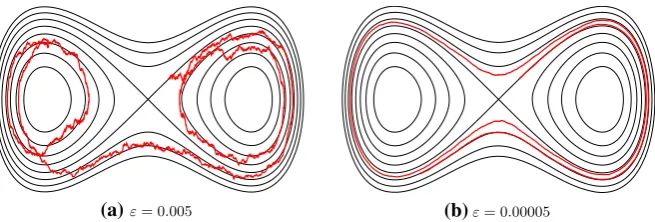
whereWtis now a 1-dimensional Wiener process. When the amplitudeεof the noise is small, the dynamics (14) splits into fast and slow components. The fast component approximately follows an unperturbed trajectory of the Hamiltonian system, which is a level set ofH. The slow component is visible as a slow modification of the value ofH, corresponding to a motion transverse to the level sets ofH. Figure1illustrates this.
Following [37] and others, in order to focus on the slow, Hamiltonian-changing motion, we rescale time such that the Hamiltonian, level-set-following motion is fast, of rateO(1/ε), and the level-set-changing motion is of rateO(1). In other words, the process (15) ‘whizzes round’ level sets ofH at rateO(1/ε), while shifting from one level set to another at rate
O(1).
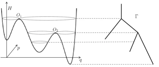
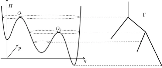
This behaviour suggests choosing a coarse-graining mapξ : R2 → , which maps a wholelevel setto a single point in a new space; because of the structure of level sets ofH, the sethas a structure that is called agraph, a union of one-dimensional intervals locally parametrized by the value of the Hamiltonian. Figure2illustrates this, and in Sect.3we discuss it in full detail.
After projecting onto the graph, the process turns out to behave like a diffusion process on. This property was first made rigorous in [37] for a system with one degree of freedom, as here, and non-degenerate noise, using probabilistic techniques. In [38] the authors con-sider the case of degenerate noise by using probabilistic and analytic techniques based on hypoelliptic operators. More recently this problem has been handled using PDE techniques [44] (the elliptic case) and Dirichlet forms [15]. In Sect.3we give a new proof, using the structure outlined in Sect.1.1.
(a)ε= 0.005 (b)ε= 0.00005
[image:9.439.58.386.480.591.2]Fig. 2 Left: HamiltonianR2(q,p)→H(q,p), Right: Graph
1.3.3 Small-noise limit of a randomly perturbed Hamiltonian system with d degrees of freedom
The convergence of solutions of (14) asε →0 to a diffusion process on a graph requires that the non-perturbed system has a unique invariant measure on each connected component of a level set. While this is true for a Hamiltonian system with one degree of freedom, in the higher-dimensional case one might have additional first integrals of motion. In such a system the slow component will not be a one-dimensional process but a more complicated object—see [40]. However, by introducing an additional stochastic perturbation that destroys all first integrals except the Hamiltonian, one can regain the necessary ergodicity, such that the slow dynamics again lives on a graph.
In Sect.4we discuss this case. Equation (14) gains an additional noise term, and reads
∂tρ= −div(ρJ∇H)+κdiv(a∇ρ)+εpρ, (16)
wherea:R2d →R2d×2d witha∇H =0, dim(Kernel(a))=1, andκ, ε >0 withκ ε. The spatial domain isR2d, d>1 with coordinates(q,p)∈Rd×Rdand the unknown is a trajectory in the space of probability measuresρ: [0,T] →P(R2d). As before the aim is to derive the dynamics asε→0. This problem was studied in [39] and the results closely mirror the previous case. The main difference lies in the proof of the local equilibrium statement, which we discuss in Sect.4.
1.4 Comparison with other work
The novelty of the present paper lies in the following.
[image:10.439.95.371.53.169.2]2. In comparison with recently developed variational-evolutionary methodsMany recently developed variational techniques for ‘passing to a limit’ such as the Sandier-Safety method based on the–∗structure [6,51,70] only apply to gradient flows, i.e. dissipative sys-tems. The approach of this paper also applies to certain variational-evolutionary systems that include non-dissipative effects, such as GENERIC systems [26,62]; our examples illustrate this. Since our approach only uses the duality structure of the rate function-als, which holds true for more general systems, this method also works for other limits in non-gradient-flow systems such as the Langevin limit of the Nosé–Hoover–Langevin thermostat [31,61,68].
3. Quantification of the coarse-graining error The use of the rate functional as a central ingredient in ‘passing to a limit’ and coarse-graining also allows us to obtain quantitative estimates of the coarse-graining error. One intermediate result of our analysis is a func-tional inequality similar to the energy-dissipation inequality in the gradient-flow setting (see (4)). This inequality provides an upper bound on the free energy and the integral of the Fisher information by the rate functional and initial free energy. To keep the paper to a reasonable length, we address this issue in details separately in a companion article [23].
We provide further comments in Sect.5.
1.5 Outline of the article
The rest of the paper is devoted to the study of three concrete problems: the overdamped limit of the VFP equation in Sect.2, diffusion on a graph with one degree of freedom in Sect.3, and diffusion on a graph with many degrees of freedom in Sect.4. In each section, the main steps in the abstract framework are performed in detail. Section5provides further discussion. Finally, detailed proofs of some theorems are given in Appendices A and B.
1.6 Summary of notation
±k j ±1, depending on which end vertexOjlies of edgeIk Sect.3.1
F Free energy (22), (46)
γ(Sect.2) Large-friction parameter
, γ(Sect.3) The graphand its elementsγ Sect.3.1
H(·|·) Relative entropy (21)
H(q,p) H(q,p)=p2/2m+V(q), the Hamiltonian
Hn n-dimensional Hausdorff measure
I(·|·) relative Fisher Information (24)
Int The interior of a set
Iε Large-deviation rate functional for the diffusion-on-graph problem (48) Iγ Large-deviation rate functional for the VFP equation (19) J J =−0I0I, the canonical symplectic matrix
L Lebesgue measure
Lμ,(Lμ)∗ Primal and dual generators Sect.1.2 M(X) Space of finite, non-negative Borel measures onX
P(X) Space of probability measures onX ˆ
ρ Push-forward underξofρ (45)
T(γ ) Period of the periodic orbit atγ ∈ (51) V(q) Potential on position (‘on-site’)
x x=(q,p)joint variable
Throughout we use measure notation and terminology. For a given topological spaceX, the spaceM(X)is the space of non-negative, finite Borel measures onX;P(X)is the space of probability measures onX. For a measureρ∈M([0,T] ×R2d), for instance, we often writeρt ∈M(R2d)for the time slice at timet; we also often use both the notationρ(x)d x andρ(d x)whenρ is Lebesgue-absolutely-continuous. We equip M(X)andP(X)with thenarrowtopology, in which convergence is characterized by duality with continuous and bounded functions onX.
2 Overdamped limit of the VFP equation
2.1 Setup of the system
In this section we prove the large-friction limitγ → ∞of the VFP Eq. (8). Settingθ =1 for convenience, and speeding time up by a factorγ, the VFP equation reads
∂tρ=Lρ∗ρ, Lν∗ρ:= −γdivρJ∇(H+ψ∗ν)+γ2
divp
ρp
m
+pρ
, (17)
where, as before,J =
0 I
−I 0
andH(q,p)= p2/2m+V(q). The spatial domain isR2d with coordinates(q,p) ∈ Rd ×Rd withd ≥ 1, and ρ ∈ C([0,T];P(R2d)). For later reference we also mention the primal form of the operatorLν∗:
Lνf =γJ∇(H+ψ∗ν)· ∇f −γ2 p
m · ∇pf +γ
2
pf. (18)
We assume
(V1) The potentialV ∈C2(Rd)has globally bounded second derivative. FurthermoreV ≥
0,|∇V|2≤C(1+V)for someC>0, and e−V ∈L1(Rd).
(V2) The interaction potentialψ∈C2(Rd)∩W1,1(Rd)is symmetric, has globally bounded first and second derivatives, and the mappingν→ν∗ψdνis convex (or equivalently non-negative).
As we described in Sect.1.1, the study of the limitγ → ∞contains the following steps:
1. Prove compactness;
2. Prove a local-equilibrium property; 3. Prove a liminf inequality.
According to the framework detailed by (1), (2), each of these results is based on the large-deviation structure, which for Eq. (17) is associated to the functional Iγ : C([0,T];P(R2d))→Rwith
Iγ(ρ)= sup f∈C1b,2(R×R2d)
R2d
fTdρT−
R2d
f0dρ0−
T
0
R2d
∂tft+Lρt ft dρtdt
−γ2 2
T
0
R2d
∇pft2dρtdt
whereLνis given in (18). Alternatively the rate functional can be written as [26, Theorem 2.5]
Iγ(ρ)= ⎧ ⎪ ⎪ ⎪ ⎨ ⎪ ⎪ ⎪ ⎩ 1 2
T
0
R2d
|ht|2dρtdt if∂tρt=Lρ∗tρt−γdivp(ρtht),forh∈L
2(0,T;L2
∇(ρ)),andρ|t=0=ρ0
+∞ otherwise,
(20)
whereLν∗is given in (17). For fixedt, the spaceL∇2(ρt)is the closure of the set{∇pϕ: ϕ∈
C∞c (R2d)}in L2(ρt), theρt-weightedL2-space. Similarly, L2(0,T;L2∇(ρ))is defined as the closure of{∇pϕ: ϕ∈Cc∞((0,T)×R2d)}in theL2-space associated to the space–time densityρ. This second form of the rate functional shows clearly howIγ(ρ)=0 is equivalent to the property thatρ solves the VFP Eq. (17). It also shows that if Iγ(ρ) > 0, then ρ is an approximate solution in the sense that it satisfies the VFP equation up to some error −γdivp(ρtht)whose norm is controlled by the rate functional.
2.2 A priori bounds
We give ourselves a sequence, indexed byγ, of solutionsργ to the VFP Eq. (17) with initial datumρtγ|t=0 = ρ0. We will deduce the compactness of the sequenceργ froma priori
estimates, that are themselves derived from the rate functionIγ. For probability measuresν, ζ onR2d we first introduce: • Relative entropy:
H(ν|ζ )=
⎧ ⎨ ⎩
R2d[f logf]dζ if ν= fζ,
∞ otherwise.
(21)
• The free energy for this system:
F(ν):=H(ν|Z−H1e−Hd x)+1
2
R2dψ∗ν
dν=
R2d
logg+H+1
2ψ∗g
gd x+logZH,
(22) whereZH =
e−Hand the second expression makes sense wheneverν=gd x.
The convexity of the term involvingψ (condition (V2)) implies that the free energyF is strictly convex and has a unique minimizerμ∈P(R2d). This minimizer is a stationary point of the evolution (17), and has the implicit characterization
μ∈P(R2d): μ(dqd p)=Z−1exp−H(q,p)+(ψ∗μ)(q) dqd p, (23)
whereZis the normalization constant forμ. Note that∇pμ= −μ∇pH = −pμ/m. We also define therelative Fisher Informationwith respect toμ(in thep-variable only):
I(ν|μ)= sup
ϕ∈Cc∞(R2d) 2
R2d
pϕ−
p m∇pϕ−
1 2|∇pϕ|
2dν. (24)
Lemma 2.1 (Equivalence of relative-Fisher-Information expressions for a.c. measures) If
ν∈P(R2d),ν(d x)= f(x)d x with f ∈L1(R2d), then
I(ν|μ)=
⎧ ⎨ ⎩
R2d
∇pf
f 1{f>0}+ p m
2f dqd p, if ∇pf ∈L1loc(dqd p),
∞ otherwise,
(25)
where1{f>0}denotes the indicator function of the set{x ∈R2d|f(x) >0}and∇pf is the
distributional gradient of f in the p-variable only.
For a measure of the formζ(dq)f(p)d p, withζ dq, the functionalIin (24) may be finite while the integral in (25) is not defined. Because of the central role of duality in this paper, definition (24) is a natural one, as we shall see below. The proof of Lemma2.1is given in AppendixA.
In the introduction we mentioned that we expectργ to become Maxwellian in the limit γ → ∞. This will be driven by a vanishing relative Fisher Information, as we shall see below. For absolutely continuous measures, the characterization (25) already provides the property
I(f d x|μ)=0 ⇒ f(q,p)= ˜f(q)exp
−p2 2m .
This property holds more generally:
Lemma 2.2 (Zero relative Fisher Information implies Maxwellian)Ifν ∈ P(R2d) with I(ν|μ)=0, then there existsσ∈P(Rd)such that
ν(dqd p)=Z−1exp
−p2 2m
σ (dq)d p,
where Z=Rde−p 2/2m
d p is the normalization constant for the Maxwellian distribution.
Proof From
I(ν|μ)= sup
ϕ∈Cc∞(R2d) 2
R2d
pϕ−
p
m · ∇pϕ−
1 2|∇pϕ|
2
dν=0 (26)
we conclude upon disintegratingνasν(dqd p)=σ (dq)νq(d p),
forσ−a.e.q: sup
φ∈C∞ c (Rd)
Rd
pφ−
p
m · ∇pφ−
1 2|∇pφ|
2
νq(d p)=0.
By replacingφbyλφ,λ >0, and takingλ→0 we find
∀φ∈Cc∞(Rd):
Rd
pφ−
p m · ∇pφ
νq(d p)=0,
which is the weak form of an elliptic equation onRd with unique solution (see e.g. [13, Theorem 4.1.11])
νq(d p)= 1
Z exp
−p2 2m
d p.
In the following theorem we give the centrala prioriestimate, in which free energy and relative Fisher Information are bounded from above by the rate functional and the relative entropy at initial time.
Theorem 2.3 (A priori bounds)Fixγ >0and letρ∈C([0,T];P(R2d))withρt|t=0=:ρ0
satisfy
Iγ(ρ) <∞, F(ρ0) <∞. (27)
Then for any t∈ [0,T]we have
F(ρt)+γ
2
2
t
0 I(ρs|μ)
ds≤Iγ(ρ)+F(ρ0). (28)
From(28)we obtain the separate inequality
1 2
R2d H dρt ≤F(ρ0)+I
γ(ρ)+log
R2de−H/2
R2de−H
. (29)
This estimate will lead to a priori bounds in two ways. First, the bound (29) gives tightness estimates, and therefore compactness in space and time (Theorem2.4); secondly, by (28), the relative Fisher Information is bounded byC/γ2and therefore vanishes in the limitγ → ∞. This fact is used to prove that the limiting measure is Maxwellian (Lemma2.5).
Proof We give a heuristic motivation here; AppendixBcontains a full proof. Given a trajec-toryρas in the theorem, note that by (20)ρsatisfies
∂tρt = −γdivρtJ∇(H+ψ∗ρt)+γ2
divpρt
p
m +pρt −γdivpρtht,
withh∈L2(0,T;L2∇(ρ)).
We then formally calculate
d
dtF(ρt)=
R2d
logρt+1+H+ψ∗ρt
−γdivρtJ∇(H+ψ∗ρt)
+γ2div
pρt
p
m +pρt
−γdivpρtht
= −γ2
R2d 1 ρt
∇pρt+ρt
p m
2+γ
R2d
ht
∇pρt+ρt
p m
≤ −γ2 2
R2d 1 ρt
∇pρt+ρt
p m
2+1
2
R2dρt
h2t,
where the firstO(γ )term cancels because of the anti-symmetry of J. After integration in time this latter expression yields (28).
For exact solutions of the VFP equation, i.e. whenIγ(ρ)=0, this argument can be made rigorous following e.g. [8]. However, the fairly low regularity of the right-hand side in (20) prevents these techniques from working. ‘Mild’ solutions, defined using the variation-of-constants formula and the Green function for the hypoelliptic operator, are not well-defined either, for the same reason: the term ∇pG·h dρthat appears in such an expression is generally not integrable. In the appendix we give a different proof, using the method of dual equations.
Equation (29) follows by substituting
F(ρt)=H
ρtZ−H1/2e−H/2d x +
1 2
R2d
H dρt+ 1 2
R2dψ∗ρt
dρt+log
R2de−H
in (28), whereZH/2:=
R2de−H/2.
2.3 Coarse-graining and compactness
As we described in the introduction, in the overdamped limitγ → ∞we expect thatρwill resemble a Maxwellian distributionZ−1exp−p2/2mσt(dq), and that theq-dependent part σwill solve Eq. (12). We will prove this statement using the method described in Sect.1.1. It would be natural to define ‘coarse-graining’ in this context as the projectionξ(q,p):= q, since that should eliminate the fast dynamics ofpand focus on the slower dynamics of
q. However, this choice fails: it completely decouples the dynamics ofq from that of p, thereby preventing the noise inpfrom transferring toq. Following the lead of Kramers [45], therefore, we define a slightly different coarse-graining map
ξγ :R2d →Rd, ξγ(q,p):=q+ p
γ. (30) In the limitγ → ∞,ξγ → ξ locally uniformly, recovering the projection onto the q -coordinate.
The theorem below gives the compactness properties of the solutionsργ of the rescaled VFP equation that allow us to pass to the limit. There are two levels of compactness, a weaker one in the original spaceR2d, and a stronger one in the coarse-grained spaceRd =ξγ(R2d). This is similar to other multilevel compactness results as in e.g. [42].
Theorem 2.4 (Compactness)Let a sequenceργ ∈C([0,T];P(R2d))satisfy for a suitable constant C>0and everyγ the estimate
Iγ(ργ)+F(ρtγ|t=0)≤C. (31)
Then there exist a subsequence (not relabeled) such that
1. ργ →ρinM([0,T] ×R2d)with respect to the narrow topology.
2. ξ#γργ → ξ#ρ in C([0,T];P(Rd))with respect to the uniform topology in time and
narrow topology onP(Rd).
For a.e. t∈ [0,T]the limitρtsatisfies
I(ρt|μ)=0 (32)
Proof To prove part 1, note that the positivity of the convolution integral involvingψand the free-energy-dissipation inequality (28) imply thatH(ρtγ|Z−H1e−Hd x)is bounded uniformly intandγ. By an argument as in [7, Prop. 4.2] this implies that the set of space–time measures {ργ :γ >1}is tight, from which compactness inM([0,T] ×R2d)follows.
To prove (32) we remark that
0≤ sup
ϕ∈C∞ c (R×R2d)
2
T
0
R2d
pϕ−
p m∇pϕ−
1 2|∇pϕ|
2dργ
t dt ≤
T
0
I(ρtγ|μ)dt
≤ C
γ2
γ→∞
−→ 0,
and by passing to the limit on the left-hand side we find
sup
ϕ∈Cc∞(R×R2d) 2
T
0
R2d
pϕ−
p m∇pϕ−
1 2|∇pϕ|
2dρ
By disintegratingρin time asρ(dtdqd p) = ρt(dqd p)dt, we find thatI(ρt|μ) = 0 for (Lebesgue-) almost allt.
We prove part 2 with the Arzelà–Ascoli theorem. For anyt∈ [0,T]the sequenceξ#γρtγ is tight, which follows from the tightness ofρtγ proved above and the local uniform convergence ξγ →ξ(see e.g. [4, Lemma 5.2.1]).
To prove equicontinuity we will show that
sup
γ >1
sup t∈[0,T−h]
sup
ϕ∈C2 c(Rd) ϕC2(Rd)≤1
Rdϕ(ξ
γ
#ρ
γ
t+h−ξ#γρ
γ
t) h→0
−−−→0. (33)
In fact, (33) is a direct consequence of the following stronger statement
Rdϕ(ξ
γ
#ρ
γ
t+h−ξ#γρ
γ
t )≤C∇ϕ∞ √
h (34)
withCindependent oft, γ andϕ. Note that (34) in particular implies a uniform 1/2-Hölder estimate with respect to theL1-Wasserstein distance.
Let us now give the proof of (34). Indeed, the boundedness of the rate functional, definition (20), and tightness ofργ imply that there exists somehγ ∈L2(0,T;L2∇(ργt))with
∂tρtγ =(Lρtγ) ∗ργ
t −γdivp(ρtγhγt). (35)
in duality withC2
b(R2d), pointwise almost everywhere in t ∈ [0,T]. Therefore for any
f ∈Cb2(R2d)we have in the sense of distributions on[0,T],
d dt
R2d
fρtγ =
R2d
γ p
m · ∇q f −γ∇qV· ∇pf −γ∇pf ·(∇qψ∗ρ
γ)
−γ2p
m · ∇pf +γ
2
pf +γ∇pf ·hγt)
dρtγ.
To prove (34), make the choice f =ϕ◦ξγ forϕ ∈Cc2(Rd)and integrate over[t,t+h]. Note that due to the specific form ofξγ =q+ p/γ the termsγmp · ∇qf andγ2mp · ∇pf cancel and therefore
Rdϕ(ξ
γ
#ρ
γ
t+h−ξ#γρ
γ
t )=
t+h
t
R2d
− ∇V(q)· ∇ϕ
q+ p γ
−(∇qψ∗ρsγ)(q)· ∇ϕ
q+ p
γ
+ϕ
q+ p
γ
+ ∇ϕ
q+ p
γ
·hγs(q,p)
dργs ds.
We estimate the first term on the right hand side by using Hölder’s inequality and growth condition (V1),
tt+hR2d∇
V(q)· ∇ϕ
q+ p
γ
dρsγds
≤ ∇ϕ∞√h
t+h
t
R2d|∇V(q)|
2dργ
s ds
1/2
≤ ∇ϕ∞√h
t+h
t
R2dC(1+V(q))ρ
γ
s ds
1/2
where the last inequality follows from the free-energy-dissipation inequality (28). For the second term we use|∇qψ∗ρsγ| ≤ ∇qψ∞and the last term is estimated by Hölder’s inequality,
tt+hR2d∇ϕ
q+ p
γ
hγs(q,p)dργsds
≤ ∇ϕ∞√h
t+h
t
R2d|
hγs|2dρsγds
1 2
≤ ∇ϕ∞√h2Iγ(ργ)12 ≤C∇ϕ ∞√h.
To sum up we have
Rdϕ(ξ
γ
#ρt+hγ −ξ#γρtγ)
≤C∇ϕ∞√h−−−→h→0 0,
whereCis independent oft, γ andϕ.
Thus by the Arzelà–Ascoli theorem there exists aν∈C([0,T];P(Rd))such thatξ#γργ → νwith respect to uniform topology in time and narrow topology onP(Rd). Sinceργ →ρ inM([0,T] ×R2d)andξγ →ξ locally uniformly, we haveξ#γργ →ξ#ρinM([0,T] ×
Rd)(again using [4, Lemma 5.2.1]), implying thatν = ξ
#ρ. This concludes the proof of
Theorem2.4.
2.4 Local equilibrium
A central step in any coarse-graining method is the treatment of the information that is ‘lost’ upon coarse-graining. The lemma below uses the a priori estimate (28) to reconstruct this information, which for this system means showing thatργ becomes Maxwellian in p as γ → ∞.
Lemma 2.5 (Local equilibrium)Under the assumptions of Theorem2.4, letργ → ρin
M([0,T]×R2d)with respect to the narrow topology andξ#γργ →ξ#ρin C([0,T];P(Rd))
with respect to the uniform topology in time and narrow topology onP(Rd). Then there exists
σ∈C([0,T];P(Rd)),σ (dtdq)=σt(dq)dt, such that for almost all t ∈ [0,T],
ρt(dqd p)=Z−1exp
−p2 2m
σt(dq)d p, (36)
where Z =Rde−p 2/2m
d p is the normalization constant for the Maxwellian distribution. Furthermoreξ#γργ →σuniformly in time and narrowly onP(Rd).
Proof Sinceργ →ρnarrowly inM([0,T] ×R2d), the limitρalso has the disintegration structureρ(dtd pdq)=ρt(d pdq)dt, withρt ∈P(R2d). From thea prioriestimate (28) and the duality definition ofIwe haveI(ρt|μ)=0 for almost allt, and the characterization (36) then follows from Lemma2.2. The uniform in time convergence ofξ#γργ impliesξ#γργ → ξ#ρ=σuniformly in time and narrowly onP(Rd)and the regularityσ ∈C([0,T];P(Rd)).
2.5 Liminf inequality
Define the (limiting) functionalI :C([0,T];P(Rd))→Rby
I(σ ):= sup g∈C1b,2(R×Rd)
RdgTdσT−
Rdg0dσ0−
T
0
Rd
∂tg
−∇V· ∇g−(∇ψ∗σ )· ∇g+g dσtdt
−1 2
T
0
Rd|∇
g|2dσtdt. (37)
Note thatI≥0 (sinceg=0 is admissible); we have the equivalence
I(σ )=0 ⇐⇒ ∂tσ =divσ∇V(q)+divσ (∇ψ∗σ )+σ in[0,T] ×Rd.
Theorem 2.6 (Liminf inequality)Under the same conditions as in Theorem2.4we assume thatργ →ρnarrowly inM([0,T] ×R2d)andξ#γργ →ξ#ρ≡ σin C([0,T];P(Rd)).
Then
lim inf
γ→∞ Iγ(ργ)≥I(σ ).
Proof Write the large deviation rate functionalIγ :C([0,T];P(R2d))→Rin (19) as
Iγ(ρ)= sup f∈C1b,2(R×R2d)
Jγ(ρ,f), (38)
where
Jγ(ρ,f)=
R2d fTdρT −
R2d f0dρ0−
T
0
R2d
∂tf +γ
p
m · ∇qf −γ∇qV· ∇pf
−γ∇pf ·(∇qψ∗ρt)
−γ2 p
m · ∇pf +γ
2
pf
dρtdt−γ
2
2
T
0
R2d
∇pf2dρtdt.
DefineA:= {f =g◦ξγ withg∈Cb1,2(R×Rd)}. Then we have
Iγ(ργ)≥sup f∈AJ
γ(ργ,f),
and
Jγ(ργ,g◦ξγ)=
R2d
gT ◦ξγdργT−
R2d
g0◦ξγdρ0γ
−
T
0
R2d
∂t(g◦ξγ)− ∇qV(q)· ∇g
q+ p
γ
+g
q+ p
γ
− ∇g
q+ p
γ
·(∇qψ∗ρtγ)(q)
dργtdt
−1 2
T
0
R2d
∇(g◦ξγ)2dρtγdt. (39)
in (39) and definingρˆγ :=ξ#γργ,Jγ can be rewritten as
Jγ(ρ,g◦ξγ)=
Rd
gTdρˆγT−
Rd
g0dρˆ0γ− T
0
Rd(∂t
g− ∇V· ∇g+g) (ζ )ρˆtγ(dζ )dt
−1 2
T
0
Rd|∇
g|2dρˆtγdt
−
T
0
R2d
∇V
q+ p
γ
− ∇V(q)
· ∇g
q+ p
γ
dργtdt
+
T
0
R2d∇
g
q+ p
γ
·(∇qψ∗ρtγ)(q)dρtγdt.
(40) We now show that (40) converges to the right-hand side of (37), term by term. Since ξ#γργ →ξ
#ρ=σnarrowly inM([0,T] ×R2d)andg∈Cb1,2(R×Rd)we have T
0
Rd
∂tg− ∇V· ∇g+g+ 1 2|∇g|
2 dρˆγ
tdt γ→∞ −−−→ T 0 Rd
∂tg− ∇V· ∇g+g+ 1 2|∇g|
2 dσ
tdt.
Taylor expansion of∇Varoundqand estimate (29) give
T
0
R2d
∇V
q+ p
γ
− ∇V(q)
· ∇g
q+ p
γ
dρtγdt
≤
≤ D2V∞∇g∞√T
T
0
R2d
p2
γ2dρ
γ
t dt
1/2
≤ C
γ
γ→∞
−−−→0.
Adding and subtracting∇g(q)·(∇qψ∗ρtγ)(q)in (40) we find
T
0
R2d∇
g
q+ p
γ
·(∇qψ∗ρtγ)(q)dργtdt =
T
0
R2d∇
g(q)·(∇qψ∗ργt)(q)dρtγdt
+
T
0
R2d
∇g
q+ p
γ
− ∇g(q)
·(∇qψ∗ρtγ)(q)dρtγdt.
Sinceργ →ρwe haveργ⊗ργ →ρ⊗ρand therefore passing to the limit in the first term and using the local-equilibrium characterization of Lemma2.5, we obtain
T
0
R2d∇
g(q)·(∇qψ∗ργ)(q)dργtdt
γ→0
−−−→
T
0
Rd∇
g·(∇ψ∗σ )dσtdt.
For the second term we calculate
0TR2d
∇g
q+ p
γ
− ∇g(q)
·(∇qψ∗ργ)(q)dρtγdt
≤
≤ D2g∞∇qψ∞ √
T
T
0
R2d
p2
γ2dρ
γ
t dt
1/2
≤ C
γ
γ→∞
−−−→0.
Therefore
T
0
R2d∇
g
q+ p
γ
·(∇qψ∗ργ)(q)dρtγdt
γ→∞
−−−→
T
0
Rd∇
g·(∇ψ∗σ )dσtdt.
2.6 Discussion
The ingredients of the convergence proof above are, as mentioned before, (a) a compactness result, (b) a local-equilibrium result, and (c) a liminf inequality. All three follow from the large-deviation structure, through the rate functionalIγ. We now comment on these.
CompactnessCompactness in the sense of measures is, both forργ and forξ#γργ, a simple consequence of the confinement provided by the growth ofH. In Theorem2.4we provide a stronger statement forξ#γργ, by showing continuity in time, in order for the limiting functional
I(σ )in (37) to be well defined. This continuity depends on the boundedness ofIγ.
Local equilibrium The local-equilibrium statement depends crucially on the structure of
Iγ, and more specifically on the large coefficientγ2 multiplying the derivatives inp. This coefficient also ends up as a prefactor of the relative Fisher Information in the a priori
estimate (28), and through this estimate it drives the local-equilibrium result.
Liminf inequalityAs remarked in the introduction, the duality structure ofIγ is the key to the liminf inequality, as it allows for relatively weak convergence ofργ andξ#γργ. The role of the local equilibrium is to allow us to replace the p-dependence in some of the integrals by the Maxwellian dependence, and therefore to reduce all terms to dependence on the macroscopic informationξ#γργ only.
As we have shown, the choice of the coarse-graining map has the advantage that it has caused the (large) coefficientsγ andγ2in the expression of the rate functionals to vanish.
In other words, it cancels out the inertial effects and transforms a Laplacian in pvariable to a Laplacian in the coarse-grained variable while rescaling it to be of order 1. The choice ξ(q,p)=q, on the other hand, would lose too much information by completely discarding the diffusion.
3 Diffusion on a graph in one dimension
In this section we derive the small-noise limit of a randomly perturbed Hamiltonian system, which corresponds to passing to the limitε→0 in (14). In terms of a rescaled time, in order to focus on the time scale of the noise, Eq. (14) becomes
∂tρε= − 1
εdiv(ρεJ∇H)+pρε. (41)
Hereρε ∈C([0,T],P(R2)), J =
0 1 −1 0
is again the canonical symplectic matrix,p
is the Laplacian in thep-direction, and the equation holds in the sense of distributions. The Hamiltonian H ∈ C2(R2d;R) is again defined by H(q,p) = p2/2m +V(q)for some potentialV :Rd →R. We make the following assumptions (that we formulate onH for convenience):
(A1) H ≥0, andHis coercive, i.e.H(x)−−−−→ ∞|x|→∞ ; (A2) |∇H|,|H|,|∇pH|2≤C(1+H);
(A3) H has a finite number of non-degenerate (i.e. non-singular Hessian) saddle points
As explained in the introduction, and in contrast to the VFP equation of the previous section, Eq. (41) has two equally valid interpretations: as a PDE in its own right, or as the Fokker-Planck (forward Kolmogorov) equation of the stochastic process
Xε=
Qε Pε
, d Xtε= 1
εJ∇H(Xεt)dt+ √
2
0 1
d Wt. (42)
For the sequel we will think ofρεas the law of the processXεt; although this is not strictly necessary, it helps in illustrating the ideas.
3.1 Construction of the graph
As mentioned in the introduction, the dynamics of (41) has two time scales when 0< ε1, a fast and a slow one. The fast time scale, of scaleε, is described by the (deterministic) equation
˙
x= 1
εJ∇H(x) inR2, (43)
whereas the slow time scale, of order 1, is generated by the noise term.
The solutions of (43) follow level sets ofH. There exist three types of such solutions: sta-tionary ones, periodic orbits, and homoclinic orbits. Stasta-tionary solutions of (43) correspond to stationary points ofH(where∇H =0); periodic orbits to connected components of level sets along which∇H =0; and homoclinic orbits to components of level sets ofHthat are terminated on each end by a stationary point. Since we have assumed in (A3) that there is at most one stationary point in each level sets, heteroclinic orbits do not exist, and the orbits necessarily connect a stationary point with itself.
Looking ahead towards coarse-graining, we defineto be the set of all connected com-ponents of level sets ofH, and we identifywith a union of one-dimensional line segments, as shown in Fig.3. Each periodic orbit corresponds to an interior point of one of the edges of ; the vertices ofcorrespond to connected components of level sets containing a stationary point ofH. Each saddle pointOcorresponds to a vertex connected by three edges.
For practical purposes we also introduce a coordinate system on. We represent the edges by closed intervalsIk⊂R, and number them with numbersk=1,2, . . . ,n; the pair(h,k) is then a coordinate for a pointγ ∈, ifkis the index of the edge containingγ, andhthe value ofH on the level set represented byγ. For a vertex O ∈, we writeO ∼ IkifO
[image:22.439.95.362.484.595.2]is at one end of edgeIk; we use the shorthand notation±k j to mean 1 ifOj is at the upper end ofIk, and−1 in the other case. Note that if O ∼ Ik1,O ∼ Ik2 andO ∼ Ik3 andh0 is the value of H at the point corresponding to O, then the coordinates(h0,k1),(h0,k2)
and(h0,k3)correspond to the same pointO. With a slight abuse of notation, we also define
the functionk : R2 → {1, . . . ,n}as the index of the edge Ik ⊂ corresponding to the component containing(q,p).
The rigorous construction of the graphand the topology on it has been done several times [15,36,37]; for our purposes it suffices to note that (a) inside each edge, the usual topology and geometry ofR1apply, and (b) across the whole graph there is a natural concept of distance, and therefore of continuity. It will be practical to think of functions f :→R
as defined on the disjoint unionkIk. A function f : →Ris then called well-defined if it is a single-valued function on(i.e., it takes the same value on those vertices that are multiply represented). A well-defined function f :→Riscontinuousiff|Ik ∈C(Ik)for everyk.
We also define a concept ofdifferentiabilityof a function f :→R. Asubgraphofis defined as any union of edges such that each interior vertex connects exactly two edges, one from above and one from below—i.e., a subtree without bifurcations. A continuous function onis called differentiable onif it is differentiable on each of its subgraphs.
Finally, in order to integrate over, we writedγ for the measure onwhich is defined on eachIkas the local Lebesgue measuredh. Whenever we write
, this should be interpreted
askI k.
3.2 Adding noise: diffusion on the graph
In the noisy evolution (42), for small but finiteε >0, the evolution follows fast trajectories that nearly coincide with the level sets ofH; the noise breaks the conservation ofH, and causes a slower drift ofXt across the levels ofH. In order to remove the fast deterministic dynamics, we now define the coarse-graining map as
ξ :R2→, ξ(q,p):=(H(q,p),k(q,p)), (44)
where the mappingk:R2 → {1, . . . ,n}indexes the edges of the graph, as above.
We now consider the processξ(Xtε), which contains no fast dynamics. For each finite ε >0,ξ(Xtε)is not a Markov process; but asε→0, the fast movement should result in a form of averaging, such that the influence of the missing information vanishes; then the limit process is a diffusion on the graph.
The results of this section are stated and proved in terms of the corresponding objectsρε andρˆε, whereρˆεis the push-forward
ˆ
ρε:=ξ#ρε, (45)
as explained in Sect.1.1, and similar to Sect.2. The corresponding statement aboutρεand ˆ
ρεis thatρˆεshould converge to someρˆ, which in the limit satisfies a (convection-) diffusion
equation on. Theorems3.2and3.6make this statement precise.
3.3 Compactness