trackeR : infrastructure for running and cycling data from GPS enabled tracking devices in R

(1)

warwick.ac.uk/lib-publications

Original citation:

Frick, Hannah and Kosmidis, Ioannis. (2017) trackeR : infrastructure for running and cycling data from GPS-enabled tracking devices in R. Journal of Statistical Software, 82 (7). pp. 1-29.

Permanent WRAP URL:

http://wrap.warwick.ac.uk/98835

Copyright and reuse:

The Warwick Research Archive Portal (WRAP) makes this work of researchers of the University of Warwick available open access under the following conditions.

This article is made available under the Creative Commons Attribution 3.0 (CC BY 3.0) license and may be reused according to the conditions of the license. For more details see:

http://creativecommons.org/licenses/by/3.0/

A note on versions:

The version presented in WRAP is the published version, or, version of record, and may be cited as it appears here.

(2)

December 2017, Volume 82, Issue 7. doi: 10.18637/jss.v082.i07

trackeR

: Infrastructure for Running and Cycling

Data from GPS-Enabled Tracking Devices in

R

Hannah Frick University College London

Ioannis Kosmidis University College London

Abstract

The use of GPS-enabled tracking devices and heart rate monitors is becoming increas-ingly common in sports and fitness activities. The trackeR package aims to fill the gap between the routine collection of data from such devices and their analyses in R. The package provides methods to import tracking data into data structures which preserve units of measurement and are organized in sessions. The package implements core in-frastructure for relevant summaries and visualizations, as well as support for handling units of measurement. There are also methods for relevant analytic tools such as time spent in zones, work capacity above critical power (known as W0), and distribution and concentration profiles. A case study illustrates how the latter can be used to summarize the information from training sessions and use it in more advanced statistical analyses.

Keywords: sports, tracking, work capacity, running, cycling, distribution profiles.

1. Introduction

Recent technological advances allow the collection of detailed data on fitness activities and on multiple aspects of training and competition in professional sport. The focus of this paper is on data collected by GPS-enabled tracking devices and heart rate monitors. Such devices are routinely used in fitness activities such as running and cycling, and also during training in sports like field hockey and football. Basic questions associated with tracking data include how often, much, or hard an individual or a group trains, and a more advanced outlook tries to explain the impact of training on athlete physiology or performance.

Tools for basic analytics are usually offered by the manufacturers of the tracking devices, such as Garmin, Polar, and Catapult, and through a wide range of applications for devices such as smartphones and smartwatches, e.g., Strava Running and Cycling GPS, Endomondo – Running & Walking, and Runtastic Running GPS Tracker. A notable open-source effort is

(3)

gold standard in terms of facilities for importing tracking data from cycling activities and for associated analytics. However, Golden Cheetah is not designed to offer general flexibility in the statistical analysis of such sports tracking data.

The R system for statistical computing (R Core Team 2017) with its ecosystem of add-on

packages provides a wide range of possibilities for the handling and analysis of tracking data.

GPS-enabled tracking devices typically record irregularly sampled spatio-temporal data.

In-frastructure for such data is provided in the trajectories package (Pebesma and Klus 2015),

which is developed around the ‘STIDF’ class of thespacetimepackage (Pebesma 2012).

How-ever, the ‘STIDF’ class does not accommodate missing values in positional or temporal

infor-mation. Since this is commonly the case in data from GPS-enabled tracking devices (e.g., sequences of missing values in the positional data because the GPS signal is temporarily lost),

a different approach is taken in package trackeR (see Section 4). Other packages that offer

tools for spatio-temporal data includeadehabtitatLT(Calenge 2006),trip(Sumner 2016) and

move(Kranstauber, Smolla, and Scharf 2017). The main focus of those packages is on animal tracking, e.g., estimation of habitat choices, and they are not directly suitable for tracking the various aspects of athlete activity.

Despite the wide range of R packages available, there is only a handful of packages specific

to sports data and their analysis. The available packages focus on topics such as sports

management (RcmdrPlugin.SM,Champely 2012), ranking sports teams (mvglmmRank,Karl

and Broatch 2015), and accessing betting odds (pinnacle.API, Blume, Jhirad, and Gassem 2017). SportsAnalytics is a package that focuses on the analysis of performance data, and currently offers only “a selection of data sets, functions to fetch sports data, examples, and

demos” (Eugster 2013). The cycleRtools package (Mackie 2016) provides functionality to

import cycling data intoRas well as tools for cycling-specific, descriptive analyses.

The trackeR package (Frick and Kosmidis 2017) aims to fill the gap between the routine collection of data from GPS-enabled tracking devices and the analyses of such data within the

Recosystem. The package provides utilities to import sports data from GPS-enabled devices,

and, after careful processing, organizes them in data objects which are organized in separate sessions/workouts and carry information about the units of measurement (e.g., distance and speed units) as well as of any data operations that have been carried out (e.g., smoothing). The package also implements core infrastructure for the handling of measurement units and for summarizing and visualizing tracking data. It also provides functionality for calculating

time in zones (e.g.,Seiler and Kjerland 2006), work capacityW0 (Skiba, Chidnok, Vanhatalo,

and Jones 2012), and distribution and concentration profiles (Kosmidis and Passfield 2015), including a few methods for the analysis of these profiles. The package is available from the

ComprehensiveRArchive Network at https://CRAN.R-project.org/package=trackeR.

Section 2 gives an overview of the package and introduces the basic objects and the

meth-ods that apply to them. Section 3 describes the importing utilities, and Section 4 details

the structure and construction of the ‘trackeRdata’ object, which is at the core of package

trackeR. Section 5 is devoted to the calculation of relevant summaries (time in zones, work capacity, distribution and concentration profiles) and the corresponding methods for

visual-ization. Section 6 and Section 7 focus on basic methods for unit manipulation as well as

smoothing and thresholding. The case study in Section 8 investigates the key features in

27 sessions through a functional principal components analysis (e.g.,Ramsay and Silverman

(4)

2. Package structure

Figures1 and 2 show a schematic overview of the package structure, split into two parts for

reading data and further operations. Squared boxes indicate objects of a particular class, diamonds indicate files of a particular format, and boxes with rounded corners represent methods that apply to those objects. The respective class and method names are given in the boxes. An arrow from an object/file type to a method indicates that the method applies to objects of the respective class; an arrow from a method to an object indicates that the method outputs objects of the respective class. A bi-directional arrow between a method and an object indicates that the method’s input and output are of the same class, such as the

methodthreshold()and objects of class ‘trackeRdata’. Arrows to or from groups of boxes

apply to each box in the group. For example, the methodchangeUnits()applies to objects of

classes ‘trackeRdataZones’, ‘trackeRdataSummary’, ‘trackeRWprime’, ‘distrProfile’, and

‘conProfile’.

Data in various formats are imported and stored in the central data object of the class ‘trackeRdata’ from which summaries for descriptive purposes or further analyses can be

derived. Methods for visualization and data handling are available for data objects and

summary objects. A list of all functionality is provided in Tables1and 2.

3. Import utilities

Package trackeR provides utilities for data in common formats from GPS-enabled tracking

devices. The family of the supplied reading functions,read*(), currently includes functions

for reading TCX (Training Centre XML), DB3 (for SQLite, used, e.g., by devices from GP-Sports) and Golden Cheetah’s JSON files. These functions read the tracking data, and return adata.framewith a specific structure.

The following code chunk illustrates the use of thereadTCX()function using a TCX file that

ships with the package and shows the name and type of variables that are present in the resulting data frame.

R> filepath <- system.file("extdata", "2013-06-08-090442.TCX",

+ package = "trackeR")

R> runDF <- readTCX(file = filepath, timezone = "GMT") R> str(runDF)

'data.frame': 1191 obs. of 9 variables:

$ time : POSIXct, format: "2013-06-08 08:04:42" ...

$ latitude : num 51.4 51.4 51.4 51.4 51.4 ...

$ longitude : num 1.04 1.04 1.04 1.04 1.04 ...

$ altitude : num 6.2 6.2 6.2 6.2 6.2 ...

$ distance : num 0 1.68 5.28 8.33 14.88 ...

$ heart.rate: num 83 84 84 86 89 93 96 98 101 102 ...

$ speed : num 0 0.594 1.416 1.928 2.614 ...

$ cadence : num NA 54 74 97 97 97 97 98 97 97 ...

$ power : num NA NA NA NA NA NA NA NA NA NA ...

(5)

readTCX

data.frame

trackeRdata

trackeRdata readContainer

readDB3

JSON file

readJSON db3 file

[image:5.595.164.439.115.325.2]

tcx file

Figure 1: Package structure – Functionality to read tracking data.

trackeRdata

summary

distributionProfile zones

trackeRdataSummary

plotRoute threshold

Wprime

trackeRdataZones

trackeRWprime

distrProfile

concentrationProfile conProfile plot

smoother

changeUnits leafletRoute

timeline nsessions

profile2fd funPCA

fda::fd trackeRfpca

[image:5.595.111.495.372.708.2]

(6)

Function Class Description

readTCX() TCX file Read TCX file

readDB3() DB3 file (SQLite) Read DB3 file

readJSON() Golden Cheetah’s JSON file Read JSON file

readContainer() TCX/DB3/JSON file Read a TCX/DB3/JSON file

readDirectory() TCX/DB3/JSON files Read all TCX/DB3/JSON files in a

4. ‘

trackeRdata

’ class

4.1. Object structure

The core object of packagetrackeRhas class ‘trackeRdata’. The ‘trackeRdata’ objects are

session-based, unit-aware and operation-aware structures, which organize the data in a list

of multivariate ‘zoo’ objects (Zeileis and Grothendieck 2005) with one element per session.

The observations within each session are ordered according to the time stamps as these are

read from the GPS-enabled tracking devices. Each ‘trackeRdata’ object has an attribute

on the measurement units of the data it holds, and, if applicable, an attribute detailing the operations, such as smoothing, it has gone through.

‘trackeRdata’ objects result from the constructor function trackeRdata(), which takes as

(8)

distinct sessions, the constructor function also performs some data processing, including basic sanity checks (for example, removing observations with negative or missing values for cumula-tive distance or speed), handling of measurement units, correction of distances using altitude

data if required, and data imputation, as discussed in Section4.5.

4.2. Constructor function

The interface of the constructor function for class ‘trackeRdata’ is

trackeRdata(dat, units = NULL, cycling = FALSE, sessionThreshold = 2, correctDistances = FALSE, country = NULL, mask = TRUE,

fromDistances = TRUE, lgap = 30, lskip = 5, m = 11)

datis the data frame containing the tracking data and units is used to specify the units of

measurement. Table3shows the currently supported units and notes the units that are used

by default whenunits = NULL. The argumentcyclingflags the data as coming from cycling

session(s) rather than running session(s). This affects the calculation ofW0 (based on power

or speed for cycling and running, respectively) and the thresholds applied before plotting the session data. The other arguments are specific to the data processing operations, which are briefly described in the following subsections.

4.3. Identifying distinct sessions

The constructor function groups the observations into sessions according to their time stamps.

Specifically, the time stamps in the data from theread*()functions are first sorted, and all

consecutive observations whose time stamps are no further apart from each other than a

specified thresholdt∗ are considered to belong to a distinct session. The value oft∗ is set via

thesessionThresholdargument of the trackeRdata() function and it defaults to 2 hours.

4.4. Distance correction using altitude data

If the distances in the data have been calculated solely based on latitude and longitude data, without taking into account the altitude, then the distance covered can be underestimated.

The correctDistances argument of the trackeRdata() function controls whether the

dis-tances should be corrected for altitude changes.

If the uncorrected distance covered at time pointti isd2,i, then settingcorrectDistances =

TRUE uses the Pythagorean theorem to correct the distance covered between time pointti−1

and time pointti to

di−di−1 =

q

(d2,i−d2,i−1)2+ (ai−ai−1)2,

wheredi andai are the corrected cumulative distance and the altitude at timeti, respectively.

If no altitude measurements are available, these are extracted fromSRTM 90m Digital

Ele-vation Datavia therasterpackage (Hijmans 2016) using the latitude and longitude

(9)

ti ti+1 t ∗ i+ h t ∗ i+ 2h t ∗ i+ 3h t ∗ i+ 4h t ∗ i+ 5h t ∗ i+ 6h t ∗ i+ 7h t ∗ i+ 9h t ∗ i+ 8h si

0 0 0 0 0 0 0 0 0

si+1

ti

si si+1

ti+1−ti> lgap

lskip lskip

ti+1

0 0

[image:9.595.82.519.75.332.2]

t∗_i t∗_i₊₁

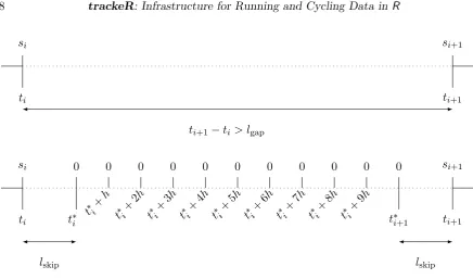
Figure 3: Illustration of the imputation process for speed withm= 11.

4.5. Imputation process

Occasionally, there is a large time difference between consecutive observations in the same session, sometimes of the order of several minutes. This can happen, for example, if the device is intentionally paused by the athlete or if the proprietary algorithm controlling the operating sampling rate of the device detects no significant change in position. For example,

in the manual of a GPS device, the Forerunner© 310XT, it is stated that“The Forerunner

uses smart recording. It records key points where you change direction, speed, or heart rate”

(Garmin Ltd. 2013). In both cases, interpolating directly to get the speed or power will lead to overestimation of the total workload within those intervals.

We assume that such intervals appear only when there is no significant work happening, and hence impute them with observations with zero speed (for running) or zero speed and power (for cycling).

Figure3shows a schematic representation of the imputation process for speed. The

parame-terslgap,mand lskip control the imputation, and can be specified via thelgap,mand lskip

arguments of thetrackeRdata() function, respectively.

If the observations at timestiandti+1are more thanlgapseconds apart, then it is assumed that

there is no significant work happening betweenti andti+1. The number of imputed records in

the interval ism, and consists of two “outer” records andm−2 “inner” records. The “outer”

records arelskip seconds apart from the existing observations forming the beginning and the

end of the interval, respectively. The “inner” records are h = (ti+1 −ti −2lskip)/(m−1) seconds apart.

The imputed records betweentiandti+1have zero speed or power, and the latitude, longitude

and altitude measurements are set to their values at timeti. All other variables are set toNA.

(10)

are as in the first and last observations, respectively, and all other variables are set to NA. The imputed records are one second apart from each other and from the first and the last observation, respectively.

After the imputation process, the cumulative distances are updated based on the imputed speeds and the time differences between consecutive observations, according to

di+1 =di+si(ti+1−ti),

where si and di denote the speed and cumulative distance at time pointti, respectively.

The following code chunk takes as input the raw data in the data frame runDFand constructs

the corresponding ‘trackeRdata’ object.

R> runTr0 <- trackeRdata(runDF)

The function readContainer()is a convenience wrapper that calls the suitable reading

func-tion and, then, trackeRdata() for the data processing and the organization of the data in a

‘trackeRdata’ object (see ?readContainerfor the available arguments). For example,

R> runTr1 <- readContainer(filepath, type = "tcx", timezone = "GMT") R> identical(runTr0, runTr1)

[1] TRUE

The function readDirectory() allows the user to read all files of a supported format in

a directory, rather than calling, e.g., readContainer() on each file separately. Using the

argument aggregate, the user can decide if all data are first combined in a data frame and

then split into sessions solely based on the time difference between consecutive observations. This way, e.g., warm-up and cool-down phases are put into the same session as the central part of training, even if they are recorded in separate container files. Alternatively, data from different container files are always stored in separate sessions.

Package trackeRships with two ‘trackeRdata’ objects containing 1 and 27 running sessions,

respectively, and which can be loaded via

R> data("run", package = "trackeR") R> data("runs", package = "trackeR")

We will use those objects for the illustrations throughout the paper.

5. Session summaries and visualization

Package trackeR provides methods for summarizing sessions in terms of scalar summaries,

the time spent exercising in specified zones, the concept of work capacity, and distribution and concentration profiles.

5.1. Visualization

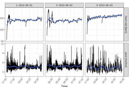
For a first visual inspection of the data, the plot() method shows by default the evolution

of heart rate and pace over the course of the selected sessions. For example, Figure 4shows

(11)

1: 2013−06−01 2: 2013−06−02 3: 2013−06−03

hear

t.r

ate [bpm]

pace [min/km]

17:30 17:45 18:00 18:15 18:30 06:30 06:40 06:50 07:00 07:10 17:50 18:00 18:10 18:20 18:30 50

100 150

3 6 9 12

[image:11.595.99.519.100.382.2]

Time

Figure 4: Heart rate and pace over the course of sessions 1–3.

R> plot(runs, session = 1:3)

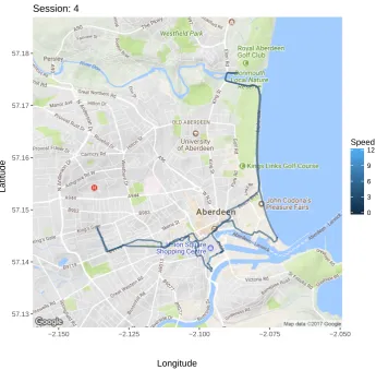
The route covered during a session can also be displayed on a static map via theplotRoute()

method. TheplotRoute()method uses theggmappackage (Kahle and Wickham 2013) and,

hence, can work with the sources and maps supported byggmap. For example, Figure5shows

the route covered during session 4 in runsusing a map downloaded from Google. Interactive

maps can be produced withleafletPlot(), using theleafletpackage (Cheng and Xie 2017).

R> plotRoute(runs, session = 4, zoom = 13)

5.2. Scalar summaries

Each session can be summarized through common summary statistics using the summary()

method. Such a session summary includes estimates of the total distance covered, the total duration, the time spent moving, and work to rest ratio. It also includes averages of speed, pace, cadence, power, and heart rate, calculated based on total duration or the time spent moving.

An athlete is considered to be moving if the speed is larger than some threshold s∗. This

threshold can be set via themovingThresholdargument of thesummary() method, and the

package assumes that anything between not moving at all and walking with a speed below

that threshold is resting. The default value formovingThresholdhas been set to 1 meter per

second, which is just below the speed humans prefer to walk at on average (1.4 meters per

(12)

57.13 57.14 57.15 57.16 57.17 57.18

−2.150 −2.125 −2.100 −2.075 −2.050

Session: 4

Longitude

Latitude

0 3 6 9 12

[image:12.595.129.475.106.445.2]

Speed

Figure 5: Route covered during session 4 on a map from Google.

The “average speed moving” is calculated as total distance covered divided by time moving while “average speed” is calculated as total distance divided by total duration. The average pace (moving) is calculated as the inverse of the average speed (moving). The work to rest

ratio is calculated as time moving divided by (total duration−time moving). The averages

for cadence, power, and heart rate (total and moving) are weighted averages with weights depending on the time difference to the next observation. These averages also need to take

into account missingness in the observations. For a variable of interestV, we can calculate a

weighted mean for the total session while accounting for missing values via

X

i

vi

∆iKi

P

i∆iKi

and its counterpart for the part of the session spent in motion via

X

i

vi

∆iKiI(si > s∗)

P

i∆iKiI(si > s∗)

,

where vi is the value of V at time pointti, Ki is 1 if vi is available, i.e., not missing, and 0

(13)

The summary() method for ‘trackeRdata’ objects returns a data frame which can be used

for further analysis. The return object is classed as ‘trackeRdataSummary’ for which several

methods are available. With theprint()method, one can set the number of digits printed for

the scalar summary statistics. The following example shows the summaries for sessions 1–2 with the default number of digits of 2 and then the summary of session 1 with 3 digits for comparison.

R> summary(runs, session = 1:2)

*** Session 1 ***

Session times: 2013-06-01 17:32:15 - 2013-06-01 18:37:56 Distance: 14130.7 m

Duration: 65.68 mins Moving time: 64.17 mins Average speed: 3.59 m_per_s

Average speed moving: 3.67 m_per_s Average pace (per 1 km): 4:38 min:sec

Average pace moving (per 1 km): 4:32 min:sec Average cadence: 88.66 steps_per_min

Average cadence moving: 88.87 steps_per_min Average power: NA W

Average power moving: NA W Average heart rate: 141.11 bpm

Average heart rate moving: 141.13 bpm Average heart rate resting: 136.76 bpm Work to rest ratio: 42.31

Moving threshold: 1 m_per_s

*** Session 2 ***

Duration: 46.07 mins Moving time: 44.13 mins Average speed: 3.42 m_per_s

(14)

Average heart rate resting: 141.16 bpm Work to rest ratio: 22.83

R> runSummary <- summary(runs, session = 1) R> print(runSummary, digits = 3)

*** Session 1 ***

Duration: 1.095 hours Moving time: 1.069 hours Average speed: 3.586 m_per_s

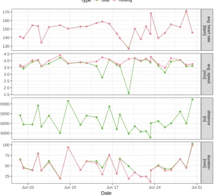
Theplot() method shows the evolution of the various summary statistics over calendar time

or over the course of the sessions. For example, the following code chunk produces Figure6.

R> runSummaryFull <- summary(runs)

R> plot(runSummaryFull, group = c("total", "moving"),

+ what = c("avgSpeed", "distance", "duration", "avgHeartRate"))

5.3. Times in zones

A common way to summarize and characterize a session is to calculate how much time was spent exercising in certain zones, e.g., heart rate zones.

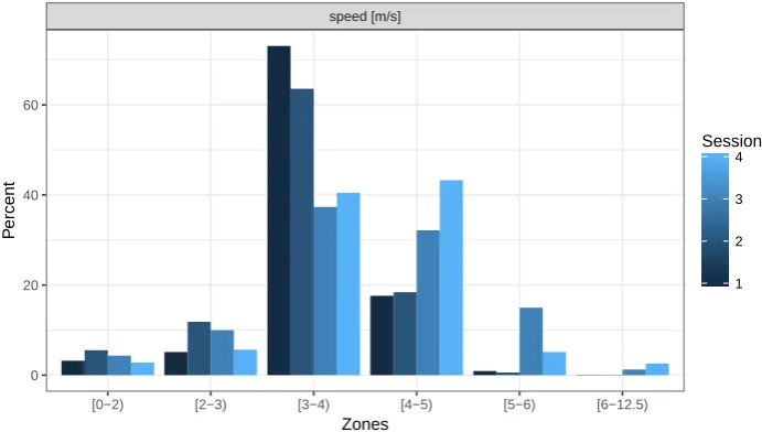
The zones() method for sessions returns an object of class ‘trackeRdataZones’ for which

methods changeUnits() and plot() are provided. The user can specify the variables, such

as heart rate and speed, and their respective zones via the arguments what and breaks,

respectively. Figure7shows a graphical representation of the zones summary, making it easier

to see that more (relative) time was spent training with high speed (> 4m/s) in sessions 3

(15)

●_● ● ● ● ● ● _● ● ● ● ● ● ● ● ● ● ● ● ● ● ● ● ● ● ● ● ●_● ● ● ● ● ● _● ● ● ● ● ● ● ● ● ● ● ● ● ● ● ● ● ● ● ● ● ● ● ● ● ● ● ● ● ● ● ● ● ●_● ● ● ● ● _● ● ● ● ● ● ● ● ●_● ● ● ● ● ● ● ● ● ● ● ● ●_● ● ● ● ● _● ● ● ● ● ● ● ● ● ● ● ● ● ● ● ● ● ● ● ● ● ● ● ● ● ● ● ● ● ● ● ● ● ● ● ● ● ● ● ● ● ● ● ● ● ● ● ● ● ● ● ● ● ● ● ● ● ● ● ● ● ● ● ● ● ● ● ● ● ● ● ● ● ● ● ● ● ● ● ● ● ● ● ● ● ● ● ● ● a vg. hear t r ate [bpm] a vg. speed [m/s] distance [m] dur ation [min]

Jun 03 Jun 10 Jun 17 Jun 24 Jul 01 130 140 150 160 170 1.5 2.0 2.5 3.0 3.5 4.0 4.5 5000 10000 15000 20000 25 50 75 100 Date

[image:15.595.101.519.112.494.2]

Type ● _total ● _moving

Figure 6: Selected session summaries for all 27 sessions.

specify the zones for a single variable: 1) in the standard way through argumentswhat and

breaks, 2) if breaks is a named list, argument what can be left unspecified and 3) if only a

single variable is to be evaluated,breaks can also be a vector.

R> runZones <- zones(runs[1:4], what = "speed",

+ breaks = list(speed = c(0, 2:6, 12.5)))

(16)

speed [m/s]

[0−2) [2−3) [3−4) [4−5) [5−6) [6−12.5)

0 20 40 60

Zones

P

ercent

1 2 3 4

[image:16.595.128.474.108.304.2]

Session

Figure 7: Zone summaries for speed of sessions 1–4.

5.4. Quantifying work capacity

The critical power model (Monod and Scherrer 1965) describes the relationship between the

power outputP and the timete to exhaustion at that power output

P = (W₀0/te) +CP (1)

in terms of two parametersW₀0 and CP. The critical power (CP) is defined by Monod and

Scherrer(1965) as “the maximum rate (of work) that [can be kept] up for a very long time

without fatigue.”Skibaet al.(2012) describeCPas “a power output that couldtheoreticallybe

maintained indefinitely on the basis of principally ‘aerobic’ metabolism.”W0 (read W prime)

represents a finite work capacity aboveCP. Skiba et al.(2012) assume thatW0 gets depleted

during exercise with a power output above CP but also replenished during exercise with a

power output of or belowCP. We denote asW0 the general concept of work capacity above

CP, and W0(t) is the state of W0 at time t. The latter is also sometimes referred to as

W0 balance at time t. Additionally, the initial state of W0 at the start of an exercise t =t0

is W₀0 = W0(t0), which is one of the parameters in the critical power model (Equation 1).

Total depletion of W₀0 results in the inability to produce a power output above CP. Thus,

knowledge of the current stateW0(t), i.e., how much of that finite work capacityW₀0 is left at

timet, is important to an athlete, particularly in a race.

While this concept is most commonly applied to cycling, where the power output is routinely

measured,Skibaet al.(2012) suggest that it can also be applied to running, substituting power

and critical power by speed and critical speed, respectively. For running, the model postulates that each runner has a finite capacity in terms of distance covered above the critical speed.

Depending on how much the runner exceeds this critical speed, the finite capacityW₀0 is being

exhausted in shorter times. Below we describe the models for depletion and replenishment of

work capacity and how they are combined in packagetrackeR.

Depletion of work capacity

(17)

and Jones (2015) assume thatW0 is depleted at a rate directly proportional to the difference

between the power output and CP

d dtW

0₍_t_{) =}₋₍_P₋_CP₎_. ₍₂₎

Solving Equation2forW0(t) gives

W0(t) =−(P−CP)t+D , (3)

whereD∈_Ris constant over t.

Suppose that the exercise over time t0 = 0 to tn = T can be split into n intervals with

breakpointst0, t1, . . . , tn such that the power output within each interval is constant, that is

P(t) =Pi fort∈[ti−1, ti), i∈ {1, . . . , n}. Then, using Equation 3, the change inW0(t) over

the interval can be expressed as

W0(ti)−W0(ti−1) =−(Pi−CP)(ti−ti−1). (4)

Replenishing of work capacity

Skibaet al. (2015) assume that the periods with a power output at or belowCP are periods

of recovery during whichW0 is replenished with a rate that depends on the difference between

CP and the power output, and the amount of W₀0 remaining, as follows:

d dtW

0₍_t_{) =}

1−W

0₍_t₎

W₀0

(CP−P). (5)

Equation 5 assumes that recovery slows down asW0(t) approaches the initial capacity W₀0.

Employing the substitution rule for integrals while solving Equation 5 and reexpressing in

terms ofW0(ti−1) (see Appendix Afor details) gives

W0(ti) =W00 − W00 −W0(ti−1)

exp

Pi−CP

W₀0 (ti−ti−1)

. (6)

Since W0(ti−1) is the amount of W00 remaining at the start of the interval [ti−1, ti), W00 −

W0(ti−1) is the amount of W00 which has been depleted prior to ti−1 and not yet been

re-plenished. Skiba et al.(2012) refer to this as W0 expended. Skiba et al. (2015) describe the

replenishing of W0 indirectly by describing how W0 expended is reduced over the course of

such a recovery interval. The exponential decay factor used in Equation6 here is the same

as their Equation 4 with only different notation. Skiba et al. (2015) use t to describe the

length of the interval, DCP = CP−Pi for the difference between critical power and power

output, andW_exp0 for the amount ofW0 previously expended. For Pi <CP, as is required for

replenishment, −DCP and Pi −CP are negative and thus the exponential factor is smaller

than 1, leading to an exponential decay as described.

Skiba et al.(2012) also assume an exponential decay of previously expended W0 to describe

replenishing W0, albeit with a different decay factor. Instead of (Pi −CP)/W00, they use

1/τW0. The relationship between the time constant of replenishing τ_W0 and the difference

between critical power and recovery power ¯P is estimated based on experimental data as

(18)

with recovery power ¯P estimated by the mean of all power outputs below CP.

Using Equation 6, i.e., the formulation of Skiba et al. (2015), the change in W0 over the

corresponding interval [ti−1, ti) can be described through

W0(ti)−W0(ti−1) = (W00−W

0

(ti−1))

1−exp

Pi−CP

W₀0 ∆i

. (7)

Work capacity at time tj

Equation4 describes the depletion of W0 (whenPi >CP) and Equation 7 describes

replen-ishment ofW0 (whenPi≤CP) over an interval [ti−1, ti). These two aspects can be combined

to describe the change over the interval as

W0(ti)−W0(ti−1) =−(Pi−CP)∆iI(Pi >CP) +

(W₀0−W0(ti−1))

1−exp

Pi−CP

W₀0 ∆i

(1−I(Pi>CP)).

The amount of W0 left at time point tj, j ∈ {1, . . . , n}, can thus be described through the

initial amount W₀0 and the changes happening in the j intervals of constant power previous

totj:

W0(tj) =W00+

j

X

i=1

(W0(ti)−W0(ti−1))

=W₀0−

j

X

i=1

(Pi−CP)∆iI(Pi>CP) + j

X

i=1

(W₀0 −W0(ti−1))

1−exp

Pi−CP

W₀0 ∆i

(1−I(Pi >CP)). (8)

W0 expended at timetj is then W00−W0(tj).

Function Wprime() can be used to calculate W0 expended by setting argument quantity

to "expended". If quantity is set to "balance", Wprime() calculates the current state

W0(t) (Equation 8). Wprime() contains implementations for Skiba et al. (2012) and Skiba

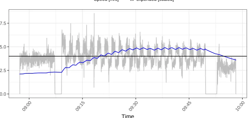
et al. (2015), which can be selected via the version argument. For example, session 11 of the example data is an interval training with a warm-up and cool-down phase. Assuming a

critical speed of 4 meters per second, the following code chunk produces Figure8, which shows

W0 expended, based on the specification of Skibaet al. (2012), along with the corresponding speed profile.

R> wexp <- Wprime(runs, session = 11, quantity = "expended", cp = 4,

+ version = "2012")

R> plot(wexp, scaled = TRUE)

During the warm-up phase speed rarely exceeds 4 meters per second andW0 expendedremains

(19)

0.0 2.5 5.0 7.5

09:00 09:15 09:30 09:45 10:00

Time

[image:19.595.98.519.114.315.2]

Speed [m/s] W' expended [scaled]

Figure 8: W0 expended in session 11.

phases and drops during the recovery phases. In the last part of the session, speeds are

mostly below 4 meters per second and W0 expended drops again.

5.5. Distribution and concentration profiles

Kosmidis and Passfield (2015) introduce the concept of distribution profiles for which the

trackeR package provides an implementation. These profiles are motivated by the need to compare sessions and use information on such variables as heart rate or speed during a session for further modeling.

For a session lastingtnseconds, the distribution profile is defined as the curve{v,Π(v)|v≥0},

where

Π(v) =

Z tn

0

I(v(t)> v)dt .

The function Π(v) is monotone decreasing and describes the time spent exercising above a

thresholdv for a variableV under consideration (e.g., heart rate or speed).

On the basis of observationsv0, . . . , vnforV, at respective time pointst0, . . . , tn, the observed

version of Π(v) can be calculated as

P(v) =

n

X

i=1

(ti−ti−1)I(vi> v).

This can subsequently be smoothed respecting the positivity and monotonicity of Π(v), e.g.,

via a shape constraint additive model with Poisson responses (Pya and Wood 2015).

The concentration profile is defined inKosmidis and Passfield(2015) as the negative derivative

of a distribution profile and is suitable for revealing concentrations of time around certain values of the variable under consideration.

Distribution profiles can be calculated using thedistributionProfile()function which

(20)

distribu-heart.rate [bpm] speed [m/s]

0 50 100 150 200 250 0 4 8 12

0 1000 2000 3000 4000 5000

Time spent abo

v

e threshold

[image:20.595.79.518.108.320.2]

1 2 3 4 Session

Figure 9: Distribution profiles for sessions 1–4.

tion profiles usingconcentrationProfile(), which returns an object of class ‘conProfile’.

Table2includes an overview of constructor functions and available methods for distribution

and concentration profiles.

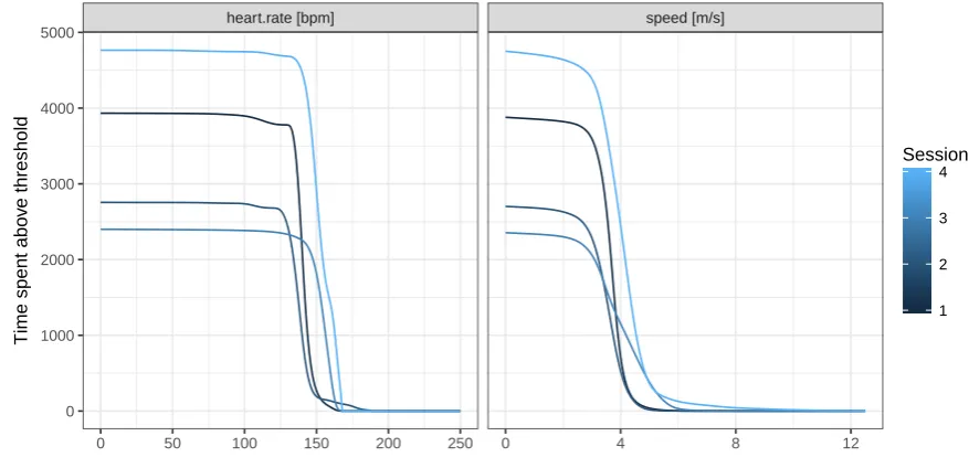
By default, distribution profiles are calculated for speed and heart rate on grids covering the ranges of [0,12.5] meters per second and [0,250] beats per minute, respectively. The following

code chunk illustrates the use of distributionProfile() and shows how users can specify

the variables for which to calculate profiles and the respective grids.

R> dProfile <- distributionProfile(runs, session = 1:4,

+ what = c("speed", "heart.rate"),

+ grid = list(speed = seq(0, 12.5, by = 0.05), heart.rate = seq(0, 250)))

R> plot(dProfile, multiple = TRUE)

The multiple argument of the plot() method determines whether to plot the profiles in

separate panels (FALSE) or overlay them in a common panel (TRUE), as in Figure 9. The

different session lengths are clearly visible in the height of the curves at 0. Amongst the distribution profiles for speed, the descent of the profile for session 3 is slower than for the other sessions. This difference is most apparent in the concentration profiles, which are shown

in Figure10 and are produced by the following code chunk.

R> cProfile <- concentrationProfile(dProfile, what = "speed") R> plot(cProfile, multiple = TRUE)

(21)

0 1000 2000 3000 4000

0.0 2.5 5.0 7.5 10.0 12.5

speed [m/s]

dtime

1 2 3 4

[image:21.595.133.472.105.336.2]

Session

Figure 10: Concentration profiles for sessions 1–4.

6. Handling units of measurement

Data objects of class ‘trackeRdata’ and all objects derived from these (‘trackeRdataSummary’,

‘trackeRdataZones’, ‘trackeRWprime’, ‘distrProfile’, and ‘conProfile’) carry an attribute

with the relevant units of measurement. ThegetUnits() method returns the units of

mea-surement for each variable and thechangeUnits()method can be used to change one or more

variables from one set of units to another. The following code chunk displays the current units

ofrun, changes the unit for speed to miles per hour, and displays the changed units.

R> getUnits(run)

variable unit

1 latitude degree

2 longitude degree

3 altitude m

4 distance m

5 heart.rate bpm

6 speed m_per_s

7 cadence steps_per_min

8 power W

9 pace min_per_km

10 duration s

R> runTr2 <- changeUnits(run, variable = "speed", unit = "mi_per_h") R> getUnits(runTr2)

variable unit

(22)

Measurement Unit(s)

Latitude Degrees (degree, default)

Longitude Degrees (degree, default)

Altitude Meters (m, default), kilometers (km), miles (mi), feet (ft)

Distance Meters (m, default), kilometers (km), miles (mi), feet (ft)

Speed Meters per second (m_per_s, default), kilometers per hour (km_per_h),

feet per minute (ft_per_min), feet per second (ft_per_s), miles per

hour (mi_per_h)

Cadence Steps per minute (steps_per_min, default for running), revolutions per

minute (rev_per_min, default for cycling)

Power Watts (W, default), kilowatts (kW)

Heart rate Beats per minute (bpm, default)

Pace Minutes per kilometer (min_per_km, default), minutes per

mile (min_per_mi), seconds per meter (s_per_m)

Duration Seconds (s), minutes (min), hours (h) – default is the largest possible unit

[image:22.595.87.525.112.330.2]

for which the duration is larger than 1

Table 3: Supported units of measurement.

2 longitude degree

3 altitude m

4 distance m

5 heart.rate bpm

6 speed mi_per_h

7 cadence steps_per_min

8 power W

9 pace min_per_km

10 duration s

Table 3 shows the variables and the corresponding units that are currently supported in

package trackeR.

If objects with different units are c()ombined in one object, the units of the first session are

applied to all other sessions. Furthermore, the changeUnits() method uses name matching

to figure out which conversion needs to be done. This allows the user to easily add support

for converting from unitOldtounitNew by authoring a function namedunitOld2unitNew.

If we wish to report the speed summaries for session 1 in runSummaryin feet per hour (not

currently supported) instead of meters per second, we need to simply provide the appropriately named conversion function as illustrated below. Note that the conversion applies to all speed summaries, i.e., to “average speed” and “average speed moving”.

R> m_per_s2ft_per_h <- function(x) x * 3937/1200 * 3600

R> changeUnits(runSummary, variable = "speed", unit = "ft_per_h")

*** Session 1 ***

[image:22.595.79.236.374.492.2]

(23)

Distance: 14130.7 m Duration: 1.09 hours Moving time: 1.07 hours

Average speed: 42349.08 ft_per_h

Average speed moving: 43350.06 ft_per_h Average pace (per 1 km): 4:38 min:sec

Moving threshold: 11811 ft_per_h

7. Thresholding and smoothing

There are instances where the data include artifacts due to inaccuracies in the GPS

measure-ments. These can be handled with thethreshold()method for objects of class ‘trackeRdata’,

which replaces values outside the specified thresholds with NA. The variables and the (lower

and upper) thresholds which should be applied for each variable can be specified through the

arguments variable, lower, and upper, respectively. An example is given in ?threshold.

The default thresholds are listed in Table 4 and, if necessary, are converted to the units of

measurement used for the ‘trackeRdata’ object.

The other option for data handling is thesmoother()method for ‘trackeRdata’ objects. This

applies a summarizing function, such as the mean or median, over a rolling window. Both

operationsthreshold() and smoother() are used in the plot() method for ‘trackeRdata’

objects. The default settings forplot() are to apply the thresholds specified in Table 4but

Variable Unit Lower threshold Upper threshold

Latitude Degrees −90 90

Longitude Degrees −180 180

Altitude Meter −500 9000

Distance Meter 0 ∞

Heart rate Beats per minute 0 250

Speed Meters per second 0 12.5 (100)

Cadence Steps (revolutions) per minute 0 ∞

Power Watts 0 ∞

Pace Minutes per kilometer 0 ∞

[image:23.595.104.500.568.721.2]

Duration Seconds 0 ∞

(24)

4: 2013−06−04

17:00 17:30 18:00

0 5 10 15 20

Time

speed [m/s]

4: 2013−06−04

17:00 17:30 18:00

0 5 10 15 20

Time

speed [m/s]

4: 2013−06−04

17:00 17:30 18:00

0 4 8 12

Time

speed [m/s]

1: 2013−06−04

17:00 17:30 18:00

0 4 8 12

Time

[image:24.595.106.500.108.409.2]

speed [m/s]

Figure 11: Speed profile of session 4 without thresholding (top left), with the default set-tings (top right), and with default thresholds as well as smoothing through a rolling median over a window of 20 observations done within the plot function (bottom left) and sepa-rately (bottom right).

not to smooth the data. The top left panel in Figure11gives an example where no thresholds

are applied and the top right panel uses default settings. The spike to over 20 meters per second in the top left panel is clearly an error in the data; the current world record for 100 meters (by Usain Bolt, August 16, 2009) is 9.58 seconds which translates to an average speed of 10.44 meters per second. The bottom panels show the effect of first applying the default thresholds and then smoothing the data through a rolling median with a window width of

20 observations, either done within the plot() method (bottom left) or explicitly via the

threshold() and smoother() methods (bottom right). The following code chunk produces

the four plots in Figure11.

R> plot(runs, session = 4, what = "speed", threshold = FALSE) R> plot(runs, session = 4, what = "speed")

R> plot(runs, session = 4, what = "speed", smooth = TRUE, fun = "median",

+ width = 20)

R> run4 <- threshold(runs[4])

R> run4S <- smoother(run4, what = "speed", fun = "median", width = 20) R> plot(run4S, what = "speed", smooth = FALSE)

(25)

Smooth-0 1000 2000 3000 4000 5000

0 4 8 12

speed [m/s]

dtime

[image:25.595.86.519.105.322.2]

5 10 15 20 25 Session

Figure 12: Smoothed speed concentration profiles for all 27 sessions.

ing a distribution profile requires a smoothing technique which respects the positivity and monotonicity of the distribution profile. This can be achieved by fitting a shape constrained

additive model with Poisson responses as implemented in thescampackage (Pya 2017). When

smoothing concentration profiles, the raw profiles are transformed to distribution profiles which are subsequently smoothed preserving the positivity and monotonicity. The smooth

concentration profiles are then derived from the smoothed distribution profiles. The plot()

methods for ‘distrProfile’ and ‘conProfile’ smooth the profiles prior to plotting by default.

8. Case study

The example data set included in the package contains 27 sessions of a single male runner in

June 2013. A visualization of scalar summaries for the sessions can be found in Figure6. The

distance covered in those sessions ranges from 2.79 km to 22.35 km, and most sessions were spent moving almost the entire time.

The code chunk below loads the data, applies thresholds, and calculates the smoothed dis-tribution profiles for the 27 sessions. The corresponding concentration profiles are shown in Figure12.

R> library("trackeR")

R> data("runs", package = "trackeR") R> runsT <- threshold(runs)

R> dpRuns <- distributionProfile(runsT, what = "speed") R> dpRunsS <- smoother(dpRuns)

R> cpRuns <- concentrationProfile(dpRunsS)

The majority of the profiles for speed concentrate around 4 meters per second. However, the curves differ in their shape (unimodal or multimodal), height, and location (revealing

(26)

PC 2 (25.1% of variability) PC 1 (66.4% of variability)

0 4 8 12

0 1000 2000 3000

speed [m/s]

[image:26.595.156.453.109.409.2]

d time

Figure 13: Harmonics 1–2 for the speed concentration profiles. Mean function (solid line) with suitable multiples of the harmonic added (dashed line) and subtracted (dotted line).

2005) can be used to explain those differences ensuring that the profiles are treated directly

as functions. Package trackeR contains a convenience function funPCA() which converts

concentration/distribution profiles to the required functional data format and performs a

functional PCA. Package trackeR can also be viewed as a stepping stone to further analysis

of tracking data with other R packages. For example, it contains a conversion function,

profile2fd(), that transforms concentration and distribution profiles to class ‘fd’ so that

users have direct access to the facilities of the fda package (Ramsay, Wickham, Graves, and

Hooker 2017) for functional data analysis.

The following code chunk shows the conversion to the required functional data format and the fitting of a functional PCA in separate steps. The PCA has four components and the share of variance is displayed in the last step.

R> library("fda")

R> cpFd <- profile2fd(cpRuns, what = "speed") R> sppca <- pca.fd(cpFd, nharm = 4)

R> varprop <- round(sppca$varprop * 100) R> names(varprop) <- 1:4

R> varprop

1 2 3 4

(27)

● ● ● ● ● ● ● ● ● ● ● ● ● ● ● ● ● ● ● ● ● ● ● ● ● ● ● −1000 0 1000 2000

25 50 75 100

duration moving [min]

PC1 ● ● ● ● ● ● ● ● ● ● ● ● ● ● ● ● ● ● ● ● ● ● ● ● ● ● ● −1000 0 1000

3.50 3.75 4.00 4.25

average speed moving [m/s]

[image:27.595.107.497.106.301.2]

PC2

Figure 14: PC1 score vs. “duration moving” (left) and PC2 score vs. “average speed mov-ing” (right).

The first two harmonics capture 91% of the variation between curves. Since further harmonics capture considerably less variation, only the first two are chosen for further inspection.

Figure13shows the mean function (solid line) and the variation captured in the two harmonics

(between the dashed and dotted lines). The first harmonic (top panel) illustrates that the most important characteristic of the concentration profiles is the relative value, which is

closely related to the overall session duration. The left panel of Figure14shows the score on

the first harmonic versus “duration moving” which is calculated as part of the scalar session

summaries. The second harmonic in the bottom panel of Figure13 shows variation along the

speed thresholds in the center of the curve. This variation can be explained well by the scalar

measure “average speed moving” as shown in the right panel of Figure14.

The concentration profiles and a functional PCA thus indicate that the two scalar summaries “duration moving” and “average speed moving” provide a good summary of the speed informa-tion in the sessions and can be used, for example, in order to incorporate speed as explanatory information in regression analyses.

Acknowledgments

We are thankful to Victoria Downie, Andy Hudson, Louis Passfield, Ben Rosenblatt, and Achim Zeileis for helpful feedback and discussions as well as providing the data that are used for the illustrations and examples in the package.

References

Blume M, Jhirad N, Gassem A (2017). pinnacle.API: A Wrapper for the Pinnacle Sports

API. R package version 2.0.9, URL https://CRAN.R-project.org/package=pinnacle.

(28)

Bohannon RW (1997). “Comfortable and Maximum Walking Speed of Adults Aged 20–79

Years: Reference Values and Determinants.”Age and Ageing,26(1), 15–19.

Calenge C (2006). “The Packageadehabitatfor theRSoftware: Tool for the Analysis of Space

and Habitat Use by Animals.” Ecological Modelling,197(3–4), 516–519. doi:10.1016/j.

ecolmodel.2006.03.017.

Champely S (2012). RcmdrPlugin.SM: Rcmdr Sport Management Plug-In. R package

version 0.3.1, URLhttps://CRAN.R-project.org/package=RcmdrPlugin.SM.

Cheng J, Xie Y (2017). leaflet: Create Interactive Web Maps with the JavaScript Leaflet

Library. Rpackage version 1.1.0, URLhttps://CRAN.R-project.org/package=leaflet.

Eugster MJA (2013). SportsAnalytics: Infrastructure for Sports Analytics. R package

version 0.2, URLhttp://soccer.R-forge.R-project.org/.

Frick H, Kosmidis I (2017). trackeR: Infrastructure for Running and Cycling Data from

GPS-Enabled Tracking Devices. Rpackage version 1.0.0, URLhttps://CRAN.R-project. org/package=trackeR.

Garmin Ltd (2013). Forerunner 310XT Owner’s Manual, Rev. G. URL http://static.

garmincdn.com/pumac/Forerunner310XT_OM_EN.pdf.

Hijmans RJ (2016).raster: Geographic Data Analysis and Modeling.Rpackage version 2.5-8,

URLhttps://CRAN.R-project.org/package=raster.

Kahle D, Wickham H (2013). “ggmap: Spatial Visualization withggplot2.” The R Journal,

5(1), 144–161.

Karl AT, Broatch J (2015). mvglmmRank: Multivariate Generalized Linear Mixed Models

for Ranking Sports Teams. Rpackage version 1.1-2, URL https://CRAN.R-project.org/ package=mvglmmRank.

Kosmidis I, Passfield L (2015). “Linking the Performance of Endurance Runners to Training and Physiological Effects via Multi-Resolution Elastic Net.” arXiv:1506.01388 [stat.AP], URLhttps://arxiv.org/pdf/1506.01388.

Kranstauber B, Smolla M, Scharf AK (2017).move: Visualizing and Analyzing Animal Track

Data. Rpackage version 3.0.1, URLhttps://CRAN.R-project.org/package=move.

Mackie J (2016). cycleRtools: Tools for Cycling Data Analysis. R package version 1.1.1,

URLhttps://CRAN.R-project.org/package=cycleRtools.

Monod H, Scherrer J (1965). “The Work Capacity of a Synergic Muscular Group.”Ergonomics,

8(3), 329–338. doi:10.1080/00140136508930810.

Pebesma E (2012). “spacetime: Spatio-Temporal Data inR.”Journal of Statistical Software,

51(1), 1–30. doi:10.18637/jss.v051.i07.

Pebesma E, Klus B (2015).trajectories: Classes and Methods for Trajectory Data.Rpackage

(29)

Pya N (2017). scam: Shape Constrained Additive Models. R package version 1.2-2, URL

https://CRAN.R-project.org/package=scam.

Pya N, Wood SN (2015). “Shape Constrained Additive Models.” Statistics and Computing,

25(3), 543–559. doi:10.1007/s11222-013-9448-7.

Ramsay JO, Silverman BW (2005). Functional Data Analysis. Springer-Verlag.

Ramsay JO, Wickham H, Graves S, Hooker G (2017).fda: Functional Data Analysis.R

pack-age version 2.4.7, URLhttps://CRAN.R-project.org/package=fda.

RCore Team (2017). R: A Language and Environment for Statistical Computing. R

Founda-tion for Statistical Computing, Vienna, Austria. URLhttps://www.R-project.org/.

Seiler KS, Kjerland GO (2006). “Quantifying Training Intensity Distribution in Elite

En-durance Athletes: Is There Evidence for an ‘Optimal’ Distribution?” Scandinavian Journal

of Medicine & Science in Sports,16(1), 49–56.doi:10.1111/j.1600-0838.2004.00418.x.

Skiba PF, Chidnok W, Vanhatalo A, Jones AM (2012). “Modeling the Expenditure and

Reconstitution of Work Capacity above Critical Power.” Medicine & Science in Sports &

Exercise,44(8), 1526–1532. doi:10.1249/mss.0b013e3182517a80.

Skiba PF, Fulford J, Clarke DC, Vanhatalo A, Jones AM (2015). “Intramuscular Determinants

of the Abilility to Recover Work Capacity above Critical Power.” European Journal of

Applied Physiology,115(4), 703–713. doi:10.1007/s00421-014-3050-3.

Sumner MD (2016). trip: Tools for the Analysis of Animal Track Data.Rpackage version

1.5-0, URLhttps://CRAN.R-project.org/package=trip.

Zeileis A, Grothendieck G (2005). “zoo: S3 Infrastructure for Regular and Irregular Time

(30)

A. Replenishment of

W

0

Assuming that power is constant, the solution of the differential equation describing the rate

of replenishment in Equation5with respect to W0(t) gives

1−W

0₍_t₎

W₀0 = exp

P −CP

W₀0 t+D/W 0

0

. (9)

Using Equation 9 over an interval [ti−1, ti) of constant power gives

1−W

0₍_t

i)

W₀0 = exp

Pi−CP

W₀0 (ti−ti−1) 1−

W0(ti−1)

W₀0

.

Hence,W0(ti) can be expressed in terms ofW0(ti−1) as

W0(ti) =W00 − W00 −W0(ti−1)

exp

Pi−CP

W₀0 (ti−ti−1)

.

Affiliation:

Hannah Frick, Ioannis Kosmidis Department of Statistical Science University College London Gower Street

London, WC1E 6BT, United Kingdom

E-mail: [email protected],[email protected]

URL:http://www.ucl.ac.uk/~ucakhfr/,http://www.ucl.ac.uk/~ucakiko/

Journal of Statistical Software

http://www.jstatsoft.org/

published by the Foundation for Open Access Statistics http://www.foastat.org/

December 2017, Volume 82, Issue 7 Submitted: 2016-02-14