A Ghost and Singularity-free
Theory
Aindri´
u Conroy
Physics
Department of Physics
Lancaster University
April 2017
A thesis submitted to Lancaster University for the degree of
Doctor of Philosophy in the Faculty of Science and Technology
Special thanks go to my parents, M´air´ın and Kevin, without whose encouragement, this thesis would not have been possible; to Emily, for her unwavering support; and to Eli, for asking so many questions.
I would also like to thank my supervisor Dr Anupam Mazumdar for his guidance, as well as my close collaborators Dr Alexey Koshelev, Dr Tirthabir Biswas and Dr Tomi Koivisto, who I’ve had the pleasure of working with. Further mention goes to Dr Claus Kiefer and Dr David Burton for fruitful discussions and to my fellow students in the Lan-caster Cosmology group - Ernestas Pukartas, Lingfei Wang, Spyridon Talaganis, Ilia Teimouri, Saleh Qutub and James Edholm - without whom, my time in Lancaster would not have been so productive and enjoyable.
Finally, I’d like to extend my gratitude to STFC and Lancaster Uni-versity for funding me throughout my studies.
List of Figures viii
1 Introduction 1
1.1 General Relativity . . . 5
1.2 Modifying General Relativity . . . 8
1.3 Infinite Derivative Theory of Gravity . . . 12
1.4 Organisation of Thesis . . . 18
2 Infinite Derivative Gravity 19 2.1 Derivation of Action . . . 19
2.2 Equations of Motion . . . 24
2.2.1 General Methodology . . . 24
2.2.2 S0 . . . 29
2.2.3 S1 . . . 30
2.2.4 S2 . . . 31
2.2.5 S3 . . . 33
2.2.6 The Complete Field Equations . . . 36
2.3 Linearised Field Equations around Minkowski Space . . . 37
2.4 Linearised Field Equations around de Sitter Space . . . 40
3 Ghost-free Conditions 46 3.1 Modified Propagator around Minkowski Space . . . 50
3.2 Examples of Pathological Behaviour . . . 53
3.3.1 Motivation from Scalar-Tensor Theory . . . 57
3.3.2 Entire functions . . . 60
3.3.3 Ghost-free condition around Minkowski Space . . . 63
4 Singularity-free Theories of Gravity 67 4.1 What is a Singularity? . . . 67
4.2 Hawking-Penrose Singularity Theorem . . . 69
4.3 The Raychaudhuri Equation and General Relativity . . . 70
4.3.1 Normalization of Timelike and Null Geodesics . . . 71
4.3.2 Derivation of Raychaudhuri Equation . . . 72
4.3.3 Convergence Conditions . . . 75
4.3.4 Rotation and Convergence . . . 76
4.3.5 Cosmological Expansion . . . 78
4.4 Defocusing Conditions for Infinite Derivative Gravity around Minkowski Space . . . 85
4.4.1 Comparison with Starobinsky Model . . . 89
4.5 Bouncing Solution . . . 90
4.5.1 Integral Form . . . 91
4.6 A simpler action of gravity. . . 94
4.7 Defocusing Conditions around de Sitter Space . . . 96
5 Conclusion 101 Appendix A Useful Identities and Notations 106 A.1 Curvature . . . 106
A.2 Bianchi Identities . . . 107
A.3 Variation of Curvature . . . 108
A.3.1 δ()R . . . 109
A.3.2 δ()Rµν . . . 110
A.3.3 δ()Rµνλσ . . . 111
Appendix C Newtonian Potential 117
Appendix D A Note on the Gravitational Entropy 121
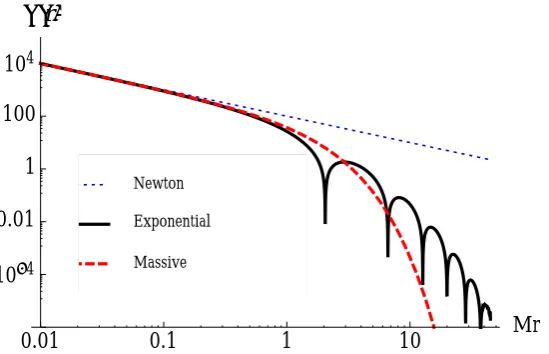
1.1 A plot of the Newtonian potential Φ(r)∼f(r)/rvs. rwheren = 1 corresponds to (1.18) with a() =e−/M2
. Higher orders of n are given by the exponential modification a() = e−(/M2)n
, whereM
has been taken to be the value of the lower bound, M = 0.004eV for illustrative purposes . . . 14
1.2 Plot showing the suppression of the gravitational potential in the
exponential model. The thick black line is the potential of the
exponential model. Few initial oscillations are visible as the
po-tential is suppressed with respect to the Newtonian 1/r behaviour
depicted by the thin blue dotted line. For comparison, we also show
the pure Yukawa suppression of massive gravity as the dashed red
line. . . 16
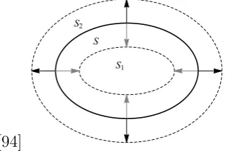
4.1 From surface S, ingoing geodesics produce a smaller surface S1
with area A1 after a time t = , while outgoing geodesics form a
larger surface S2 with area A2. This is the behaviour of ingoing
and outgoing expansions in a flat spacetime and the surfaces S1
4.2 A conformal diagram of a Big Bang cosmology with local inflation. Shaded regions are antitrapped and white regions are normal sur-faces. A patch begins to inflate at cosmic timet fromO toQwith inflationary size xinf, where the line OP borders the apparent in-flationary horizon. The arrow depicts an ingoing null ray entering an antitrapped region from a normal region, which is prohibited under the convergence condition (4.23). The inflationary patch
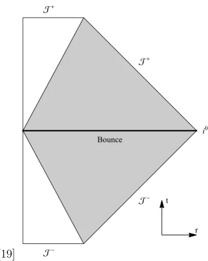
OQ may indeed be extended into the antitrapped region so that no such violation occurs. . . 83 4.3 A conformal diagram depicting a bouncing cosmology, seen as an
Chapter 2
• “Generalized ghost-free quadratic curvature gravity”
T. Biswas, A. Conroy, A. S. Koshelev and A. Mazumdar.
Class. Quant. Grav. 31, 015022 (2014), arXiv:1308.2319 [hep-th]
Chapter 3
• “Nonlocal gravity in D dimensions: Propagators, entropy, and a bouncing cosmology”
A. Conroy, A. Mazumdar, S. Talaganis and A. Teimouri.
Phys. Rev. D 92, no. 12, 124051 (2015) arXiv:1509.01247 [hep-th]
Chapter 4
• “Defocusing of Null Rays in Infinite Derivative Gravity”
A. Conroy, A. S. Koshelev and A. Mazumdar.
JCAP 1701, no. 01, 017 (2017) arXiv:1605.02080 [gr-qc]
• “Geodesic completeness and homogeneity condition for cosmic inflation”
A. Conroy, A. S. Koshelev and A. Mazumdar.
Phys. Rev. D 90, no. 12, 123525 (2014) arXiv:1408.6205 [gr-qc]
Abstract D
• “Wald Entropy for Ghost-Free, Infinite Derivative Theories of Gravity”
A. Conroy, A. Mazumdar and A. Teimouri.
Introduction
Just over a century has passed since Einstein first presented his work on General Relativity (GR) to the Prussian academy, ushering in a new paradigm for modern physics. In the intervening years, Einstein’s remarkable theory has withstood the
enormous advancements in experimental physics and observational data - with each new discovery adding further weight to this colossus of scientific endeavour. General Relativity is not only considered one of mankind’s greatest scientific discoveries but one of the most significant intellectual achievements in human history. Outside of the scientific sphere, the influence of relativity can be found in the arts – whether it be in the work of existential playwright Luigi Pirandello, who played with traditional notions of the observer, or Pablo Picasso, whose distorted perspective was reportedly inspired by the idea of displaying a fourth dimension on canvas [1]. That is not to say, however, that Einstein’s gravity does not have its shortcomings, specifically in constructing a quantum field theory of gravity; as well as describing a viable theory of gravity, which is devoid of singularities.
the continuous Lorentzian manifold of GR to be an approximation of a discrete
spacetime structure [7]. A common thread running through these fundamentally
different approaches is the presence ofnon-locality, where interactions occur not
at a specific spatial point but over a (finite) region of space [8],[9][10],[11]. Indeed, non-locality arising from infinite derivative extensions of GR has been shown to
play a pivotal role in the more classical context of resolving the cosmological
singularity problem, [12],[13],[14],[15],[16][17],[18],[19],[20][21],[22], which is our
focus here.
The concept of singularities is a particularly confounding, yet intriguing, topic.
Often casually referred to as a ‘place’ where curvature ‘blows up’, or a ‘hole’ in the
fabric of spacetime – the concept of a singular spacetime raises thorny questions
for a physicist. If a singularity is a ‘hole’ in the fabric of spacetime, can it be
said to exist within the framework of spacetime? Could we not simply omit the
singularity from our spacetime manifold? On the other hand, if the singularity
does indeed exist within the spacetime, what does it mean to have a ‘place’ within
this framework where the normal physical laws that govern the universe no longer
apply? The difficulty lies in a unique characteristic of general relativity in that it
is formulated without stipulating the manifold and metric structure in advance.
This is in contrast to other physical theories, such as special relativity, where these
are clearly defined. As such, without a prescribed manifold, it is not possible to
discuss the concept of ‘outside’ the manifold. Neither can one consider the notion of a ‘place’ where curvature may ‘blow up’ as this ‘place’ is undefined a priori
[23],[24]. Such intuitive inconsistencies lead many to believe that singularities are
not physically present in our Universe and that GR’s admittance of singularities
is evidence of the need to extend this powerful gravitational theory. In this way,
we see the Einstein-Hilbert action of GR as a first approximation of a broader
theory.
Proposals for modifying general relativity have been put forward since
al-most its inception. Early examples include Eddington’s reformulation of GR in
along with Maxwell’s equations, giving hopes for a unified theory of gravitation and electromagnetism. While mathematically elegant, the Kaluza-Klein model predicted an additional massless scalar field which is in conflict with experimental
data. Despite this, the technique of introducing higher dimensions is considered to be a great influence on the development of string theory [26]. Much later, in 1977, Stelle proposed a fourth order extension of GR [27],[28], given by
L∼R+f1R2+f2RµνRµν+f3RµνσλRµνσλ. (1.1)
Fourth order or four-derivative gravity – so-called as each term in the resulting field equations contains four derivatives of the metric tensor – is a somewhat natural extension of gravity, if seen as a generalisation of the Gauss-Bonnet term, which appears in Lovelock gravity [29],[30], and is trivial in four dimensions. We
return to this point briefly in Section 1.2. What is remarkable, however, is that Stelle found that such theories are perturbatively renormalizable, leading to a boon in the field of quantum gravity [31],[32],[27],[33]. A particular instance of fourth order gravity, known as the Starobinsky model [34], with
L∼R+f0R2, (1.2)
created further interest due to its description of successful primordial inflation. Starobinsky’s initial idea was to formulate a gravitational theory that mimics the
behaviour of the cosmological constant. For sufficiently large R this model does precisely that through the R2 term, leading to the formation of the large scale structures we see in the Universe today. The quadratic curvature term becomes less dominant as the theory moves away from the Planck scale, signalling the end of inflation.
Infinite derivative theories, in contrast, have the potential to describe a the-ory that is free of ghosts by modifying the graviton propagator via an exponent of an entire function [15],[16]. This exponential suppression of the propagator results in an exponential enhancement of the vertex factors of the relevant Feyn-man diagrams [38]. Furthermore, the nature of this modification is such that one can always construct a modified propagator that contains no additional de-grees of freedom, other than the massless graviton, so that negative residues will not propagate [15],[16],[17],[18],[19],[20],[21],[22]. Infinite derivative extensions of relativity have been shown to display improved behaviour in the UV, in terms of alleviating the 1/r behaviour of the Newtonian potential [16], and curtailing quantum loop divergences [39],[40]. Recent progess has also been made in terms of the resolution of the black-hole singularity problem [41] and a study of the dynamical degrees of freedom via Hamiltonian analysis [42]. Infinite derivatve extensions of relativity also allow for the formulation of non-singular cosmologies [18],[19], which we cover extensively in Chapter 4, and forms the basis of the present work. In simple terms, theobjective of this thesis is
To present a viable extension of general relativity, which is free from
cosmological singularities.
A viable cosmology, in this sense, is one that is free from ghosts, tachyons or exotic matter, while staying true to the theoretical foundations of General Relativity such as the principle of general covariance, as well as observed phenomenon such as the accelerated expansion of the universe and inflationary behaviour at later times [43].
has suffered setbacks following the discovery of the cosmic microwave background
in 1965 [46], though some proponents of “quasi-steady” models remain [47].
Another popular resolution to the cosmological singularity problem is the
bouncing universe model, where the Big Bang singularity is replaced by a Big
Bounce [48],[49]. Such a cosmology issues from a scale factor that is necessarily
an even function [13],[50]. Although the term “Big Bounce” was not popularised
until the 1980s [51], such cosmologies have a long history of interest, stretching
back to the time of Willem de Sitter [52].
Unlike bouncing models of the universe, we make no such stipulations on
the nature of the cosmological scale factor a priori, preferring to confront the
cosmological singularity problem by employing the Raychaudhuri equation (RE)
[53],[54], first devised in 1955 [55]. The RE is a powerful identity, which relates the
geometry of spacetime to gravity, so that the behaviour of ingoing and outgoing
causal geodesic congruences can be understood in a gravitational context. If
these geodesics converge to a point in a finite time, they are called geodesically
incomplete, resulting in a singularity in a geometrically-flat or open cosmology
[56],[57],[58],[24],[59],[43],[60]. Similarly, one can deduce the physical conditions,
whereby these causal ‘rays’ diverge, ordefocus, as a means of describing a viable
non-singular cosmology.
We will return to these points shortly, but it is perhaps instructive to first
review some of the central tenets that GR relies upon - detailing what it is about
GR that makes it such a special theory, before expanding on the need to modify
or extend GR.
1.1
General Relativity
The Weak Equivalence Principle
A key stepping stone in the formulation of GR was Einstein’s Equivalence
Prin-ciple, which states that, locally, inertial and gravitational mass are equivalent.
Roughly speaking, this is tantamount to saying that the physics of a freely falling
gravitational field, which is why this principle is sometimes referred to as the uni-versality of free fall. In terms of Newtonian gravity, inertial massmi is the form of
mass that makes up Newton’s second law of motion, i.e. F =mia, whereas
grav-itational mass mg appears in Newton’s Law of Gravitation, F =
Gmg1mg2
r2 . The
equivalence of these two forms of mass can be seen as a direct result of Galileo’s
leaning tower of Pisa experiment, where balls of two different masses reach the ground at the same time, in that the acceleration due to gravity is independent
of the inertial or gravitational mass of the body in question. This simple insight led Einstein to formulate a theory where gravity is not described as a force but
by geometry - by the curvature of spacetime [61],[24],[62].
“All uncharged, freely falling test particles follow the same trajectories
once the initial position and velocity have been prescribed” [25]
- The Weak Equivalence Principle (WEP)
A fine-tuning of the Einstein Equivalence Principle led to the Weak Equivalence Principle, stated above, which has been tested rigorously over the years, beginning
with the experiments of Lor´and E¨otv¨os in 1908. Current experiments place the constraint on the WEP and therefore any viable relativistic theory to be
η= 2|a1−a2|
|a1+a2|
= (0.3±1.8)×10−13. (1.3)
Here, beryllium and titanium were used to measure the relative difference in
acceleration of the two bodies, a1 and a2, towards the galactic centre. This is
considered to be a null result, wholly consistent with General Relativity [25].
Principle of General Covariance
Another central tenet of General Relativity, which was instrumental in the
formu-lation of GR and is perhaps more relevant to the present work, is the principle of general covariance. General covariance insists that each term making up a
gravi-tational action will transform in a coordinate-independent way. The principle was first struck upon by Einstein when formulating the theory of special relativity,
frames. Furthermore, the universal nature of the tensor transformation law
of-fered a simple means of rendering physical equations generally covariant. That is
to say that any gravitational action expressed in terms of tensors (and covariant
operators) would be a generally covariant action. Reformulating gravity in terms
of tensors - with the graviton represented by a type (2,0) metric tensor - allowed for a gravitational theory to be described by curvature alone. This proved to be
the cornerstone of General Relativity and any valid modification or extension of
GR should conform to this principle.
Gravitational Action
We have now established that the central idea behind GR, as opposed to the
Newtonian theory of gravitation, is that what we perceive as the force of gravity
arises from the curvature of spacetime. Mathematically, this can expressed by
the gravitational action which defines the theory
S = 1 2
Z
d4x√−g MP2R−2Λ, (1.4)
known as the Einstein-Hilbert action, where MP =κ−1/2 =
q
~c
8πG is the Planck
mass, with ~ = c = 1 (natural units); R is the curvature scalar, defined in Appendix A.1, the determinant of the metric tensor is given byg = det(gµν); and
the cosmological constant is Λ, which we take to be of mass dimension 4 in our
formalism. Variation of the action with respect to the metric tensor gives rise to
the famous Einstein equation
MP2Gµν+gµνΛ =Tµν, (1.5)
whereGµν ≡Rµν−12gµνRandTµν are the Einstein and energy-momentum tensors
1.2
Modifying General Relativity
Despite the phenomenal success of the theory of relativity, outstanding issues
remain, which suggests that the theory is incomplete. As mentioned in the
intro-duction, one of these issues concerns the construction of a theory which marries
quantum field theory (QFT) with GR. This has been an open question in
mod-ern physics since almost the inception of QFT in the 1920s, but gained particular
traction with the rise of string theory in the 1960s and 70s. A more classical
shortcoming of GR arises from its admittance of singularities, where the normal
laws of physics can be said to ‘break down’. We now discuss how GR cannot
de-scribe a viable, non-singular cosmology, in order to motivate the need to extend
the theory.
Singularities
The Cosmological Singularity Problem is the focal point of the present text, with
Chapter 4 devoted to the description of a stable,extended theory of relativity
de-void of an initial singularity. The requirement of extending GR in order to ade-void a
Big Bang singularity can be seen by referring to the Raychaudhuri equation (RE),
see Section (4.3) for full details. The RE is a powerful identity which relates the
geometry of spacetime to gravity, so that the behaviour of ingoing and outgoing
causal geodesic congruences can be understood in a gravitational context. From
this, one can deduce the necessary conditions whereby ingoing causal geodesics
will converge to the same event in a finite time. This convergence is known as
geodesic incompleteness and a freely falling particle travelling along this geodesic
will, at some finite point in time, cease to exist. We call such a spacetimesingular
and the associated condition is known as the convergence condition [23].
Here, we merely outline the convergence conditions in GR, which are discussed
in greater detail in Chapter 4, as a means of motivating the need to modify or
extend the theory. From the RE, one can deduce that a spacetime will be
null-geodesically incomplete if either of the following conditions are met [58],[59],[63],
dθ dλ +
1 2θ
2
Leaving aside the left hand inequality for the moment, which describes the con-vergence condition in terms of geometric expansion, let us focus on the right hand
inequality within the framework of GR. From the Einstein-Hilbert action (1.4), we derive the Einstein equation (1.5), while also noting that null geodesic congru-ences vanish when contracted with the metric tensor, according togµνkµkν = 0.
Thus,
Rµνkµkν =κTµνkµkν, (1.7)
must be positive in order to retain the null energy condition (NEC), see Appendix
(B), and to avoid the propagation of potentially exotic matter [64],[65]. Thus, in GR we are left with the choice of either accepting singularities or accepting potentially non-physical matter. As neither option is desirable, we conclude that
GR must be extended in order to describe a viable non-singular cosmology.
Lovelock’s Theorem
An important theorem in both the formulation of GR and concerning any valid extension of the theory isLovelock’s Theorem[25],[30]
Theorem 1.2.1 (Lovelock’s Theorem). The only possible second-order
Euler-Lagrange expression obtainable in a four-dimensional space from a scalar density
with a Lagrangian dependent on the metric tensor (i.e. L=L(gµν)) is
Eµν =√−g(αGµν+gµνλ), (1.8)
where both α and λ are constants
This is a remarkable result when one considers that by taking λ = Λ, this is precisely the Einstein equation in the presence of the cosmological constant, modified only by the constantα. What this theorem says is that any gravitational theory in a four-dimensional Riemannian space, whose subsequent field equations are of second order or less will be defined solely by the Einstein equation. As
that also reproduces the same result, and this is given by
L=√−g(αR−2Λ)+β√−g R2−4RµνRµν+RµνλσRµνλσ
+γµνλσRαβµνRαβλσ.
(1.9) In four dimensions the final two terms do not contribute to the field equations. Whereas this is true for the final term in any number of dimensions, the second term is what as known as the Gauss Bonnet term and is non-trivial in theories of dimensions higher than four.
What Lovelock’s theorem means for modified theories of gravity is that, if we assume that we want to describe a generally covariant, four-dimensional, metric-tensor-based theory of gravity, whilst retaining the variational principle, we have two options:
1. Extend our approach into field equations that contain higher than second
order derivatives and/or
2. Allow a degree of non-locality to enter the system.[25]
Examples of Modified Theories
Fourth Order Gravity
We have already noted that the action (1.9) is the most general action that reproduces the Einstein-field equation. A generalisation of the Gauss-Bonnet term
GGB =R2−4RµνRµν+RµνλσRµνλσ, (1.10)
forms the basis for what is calledFourth Order Gravity,
L=R+f1R2+f2RµνRµν+f3RµνσλRµνσλ. (1.11)
f(R)-gravity
Perhaps the simplest generalisation of the Einstein-Hilbert action (1.4) comes in
the form off(R)-gravity, where the curvature scalarRis replaced by an arbitrary functionf acting on the curvature R,
S = M
2
P
2
Z
d4x√−gf(R). (1.12)
By varying with respect to the metric tensor, we can then read off thef(R) field equations
κTµν =f0(R)Rµν−
1
2gµνf(R) +gµνf
0
(R)− ∇µ∇νf0(R), (1.13)
wheref0 =∂f(R)/∂R, =gµν∇
µ∇ν and using δf(R) = f0(R)δR.
Starobinsky Model
The Starobinsky model is a particular instance off(R)-gravity with
f(R) = R+c0R2, (1.14)
for some real constant c0. Recall that Starobinsky’s initial idea was to formulate
a gravitational theory that mimics the behaviour of the cosmological constant,
leading to successful primordial inflation. This model will be of particular interest
when discussing the defocusing conditions of infinite derivative theory, where it is
found that the Starobinsky model struggles to pair successful inflation with the
1.3
Infinite Derivative Theory of Gravity
The most general infinite derivative action of gravity that is quadratic in curvature
was first derived in [15], and was found to take the form
S =
Z
d4x √
−g
2
MP2R+λRF1()R+λRµνF2()Rµν +λCµνλσF3()Cµνλσ
,
(1.15)
where the form factorsFi() are given by
Fi() =
∞ X
n=0
fin(/M)
n
(1.16)
and M is the scale of non-locality. In this form, we can see this as a natural generalisation of fourth order gravity to include all potential covariant operators
in accordance with the principle of general covariance. The above action has been studied extensively in terms of the modified propagator [36]; Newtonian potential
[66],[16]; gravitational entropy [67],[68]; loop quantum gravity [39],[40],[38]; and indeed, singularity avoidance [18],[19],[41]. We will summarise some relevant
re-sults shortly. Firstly, however, let us briefly expand on the notion of non-locality, alluded to in the introductory paragraphs.
Non-locality
We stated earlier that a consequence of Lovelock’s theorem is that a valid modi-fied theory of gravity must include derivatives that are of second order or higher
and/or allow a degree of non-locality. In this sense, the action (1.15) conforms
to both of Lovelock’s stipulations in that it is both of higher order than 2 and non-local, so that (1.15) can be understood as an effective action [15],[69]. A
theory featuring an infinite series of higher-derivative terms, such as the infi-nite derivative gravity (IDG) theory introduced above, and derived in Chapter 2,
yields non-local interactions and a relaxation of the principle of locality, which, in simple terms, states that a particle may only be directly influenced by its
immediate surroundings.
and found to potentially alleviate divergences in the UV, by allowing for the super-renormalizability of the theory [70],[71],[39]. Non-local objects, such as strings and branes, are a fundamental component of string theory, while the formulation of Loop Quantum Gravity is based on non-local objects, such as Wilson Loops [40]. The IDG theory, defined by the action (1.15) was inspired by the non-locality that arises from exponential kinetic corrections, common in string theory, see [15],[26]. In terms of the Feynman diagrams, non-local interactions result in an exponential enhancement of the vertex operator, meaning that interaction does not take place at this point, as in a local theory [27, 39, 72]. Note also, that while a series of infinite derivatives is a common feature of non-local theories, it is not true to say that this is a defining characteristic. For example, massive gravity theories which modify GR in the infrared, e.g. ∼ 1
2R, are indeed non-local but
have finite orders of the inverse D’Alembertian [73],[74],[75],[76],[77].
Summary of Results
In this section, we summarise some of relevant results, achieved within an infinite derivative gravitational framework, that are not explicitly covered in the
subse-quent chapters.
Newtonian Potential
In [16], the Newtonian potential was studied around the weak field limit of the action (1.15). In this case, the modified propagator was modulated by an overall factor of a() = e−/M2, where M is the scale of modification. The exponen-tial nature of this function was invoked in order to render the theory ghost and tachyon free, which is covered in detail in Chapter 3. For a theory with modified propagator Π, given by
Π = 1
a(−k2)ΠGR, (1.17)
where ΠGR is the physical graviton propagator and→ −k2 in Fourier space on
a flat background, the Newtonian potential Φ(r) was found to be
Φ(r)∼ mπ
2M2
Pr
Erf(rM
Here, we observe that the potential contains the familiar 1/r divergence of GR, modulated by an error function Erf(r). At the limit r → ∞ 1, erf(r)/r → 0
returning flat space. Furthermore. at the limit r → 0, the potential converges to a constant, thus ameliorating the 1/rdrop-off of GR and displaying improved behaviour in the UV. The explicit calculation can be found in Appendix C. The behaviour of the Newtonian potential in an IDG theory was further expanded upon in [66], where a more general ghost-free form factor
a() = e−γ(/M2) (1.19)
was studied, where γ is some entire function. In this case, identical limits were observed atr→ ∞. Furthermore, using laboratory data on the gravitational po-tential between two masses at very small distances, the lower limitM > 0.004eV
was placed on the the scale of modification.
GR n=1 n=2 n=16
2.×10-5 5.×10-5 1.×10-4 2.×10-4 5.×10-4
1×10⁴
2×10⁴
5×10⁴
r(metres)
f
(
r
)/
r
(
metres
-1 )
[image:26.595.124.491.402.608.2][66]
Figure 1.1: A plot of the Newtonian potential Φ(r)∼f(r)/rvs. r wheren= 1
corresponds to (1.18) with a() = e−/M2. Higher orders of n are given by the
exponential modification a() = e−(/M2)n, where M has been taken to be the
value of the lower bound, M = 0.004eV for illustrative purposes
1Alternatively, if we take M → ∞, which is the limit to return IDG to a local theory, we
Entropy
The gravitational Wald entropy for IDG theories was investigated across two papers in [67] and [68]. It was found in [67] that the gravitational entropy ac-counting for the UV-modified sector vanishes around an axisymmetric black-hole metric when one requires that no additional degrees of freedom are introduced in the linear regime – a condition which results in a ghost-free theory. The resulting entropy was given simply by the famous area law,
SWald = Area
4G . (1.20)
In [68], the analysis was extended to consider the gravitational entropy around
an (A)dS metric, where a lower bound on the leading order modification term was calculated which precludes non-physical spacetimes characterised by nega-tive entropy. This bound was found to have cosmological significance in terms of avoiding singularities around a linearised de Sitter background. See Section D for an outline of this result.
Quantum Loop Gravity
Quantum aspects have been studied for IDG theories, specifically from the point of view of a toy model, see [39]. Here, explicit 1-loop and 2-loop computations were performed where it was found that, at 1-loop, a divergence arises. However, counter terms can be introduced to remove this divergence, in a similar fashion to loop computations in GR. Furthermore, at 2-loops the theory becomes finite. The article [39] then suggests a method for rendering arbitrary n-loops finite.
Modifications in the Infrared
The present work focuses solely on modifications to GR in the UV. Recently, however, interest has been generated in the field of non-local modifications in the infrared (IR). Such theories are characterised by the presence of inverse D’Alembertian (1/) corrections in the gravitational action. Most notably, re-cent work has re-centred on the idea of constructing a theory of gravity which confers a non-zero mass upon the graviton, known as massive gravity. Massive gravity theories are formulated via a m2gr
0.01 0.1 1 10 Mr 10-4
0.01 1 100 104
FHrL
[image:28.595.168.443.140.317.2]Massive Exponential Newton
Figure 1.2: Plot showing the suppression of the gravitational potential in the exponential model. The thick black line is the potential of the exponential model. Few initial oscillations are visible as the potential is suppressed with respect to the Newtonian 1/r behaviour depicted by the thin blue dotted line. For comparison, we also show the pure Yukawa suppression of massive gravity as the dashed red line.
wheremgr is the mass of the massive graviton. Such theories have been explored
in a number of papers as a means to explain the proliferation of dark energy in
the Universe [73],[74],[77],[76],[78][79].
In [75], the full non-linear field equations for a generalised action made up
of an infinite series of inverse D’Alembertian operators was derived for the first
time. The gravitational action can be formulated by replacing the form factors
Fi() in (1.15) with
¯
Fi() =
∞ X
n=1
f−n(M2/)n. (1.21)
Similar methods to [16] were employed in order to derive the modified Newtonian
potentials, with the added complexity that models with an additional degree of
freedom in the scalar propagating mode were not excluded, i.e. a6=cin Appendix C, resulting in two Newtonian potentials. An upper bound was placed on the
ratio of these potentials, known as the Eddington parameter, via the Cassini
tracking experiment and various models were analysed as a means of explaining
1.4
Organisation of Thesis
The content of the thesis is organised as follows:
Chapter 2: This chapter begins with a derivation of the most general, generally covari-ant, infinite derivative action of gravity that is quadratic in curvature, before moving on to the main focus of the chapter: the highly non-trivial task of attaining the full non-linear field equations. The general methodology is outlined before moving on to the explicit calculation. Finally the linearised field equations are derived around both Minkowski and de Sitter spacetimes for later use in the context of ghost and singularity free cosmologies.
Chapter 3: The general ghost and tachyon criteria that a viable theory must conform to are established, with specific examples of pathological behaviour given. The correction to the graviton propagator from the infinite derivative extension is attained, as are the ghost-free conditions around Minkowski space.
Infinite Derivative Gravity
2.1
Derivation of Action
Having introduced the concept of infinite derivative gravity theories and some
of the progress made in the area, our goal here is to derive the most general,
generally covariant infinite derivative action of gravity, with a view to formulating the associated equations of motion. Following this, in Chapter 3, we will use the
field equations to understand the nature of the modified propagator.
We begin by inspecting the fluctuations around a given background up to quadratic order inh, according to
gµν =ηµν +hµν. (2.1)
For presentation purposes, we have restricted the background metric to that
of the Minkowski spacetime as in [16], while the derivation has been repeated
in the more general framework of maximally symmetric spacetimes of constant curvature, i.e. Minkowski or (Anti) de Sitter space, in [80],[81]. In principle, it
should be possible to relax this restriction on the background metric further to
any background metric with a well-defined Minkowski limit, with this latter point
required to eliminate potentially singular non-local terms.
metric-tensor-based gravitational action, with a well-defined Minkowski limit,
may be expressed in the following generic form
S =
Z
d4x√−g
"
P0+
X
i
Pi
Y
I
(OiIQiI)
#
, (2.2)
where P and Q are functions of Riemannian curvature and the metric tensor,
while the operator O is made up, solely, of covariant operators, in accordance
with general covariance.
Our goal is to inspect fluctuations around Minkowski space up to quadratic
order. To this end, following closely to [80],[81],[16],[15], we may recast (2.2) into
the following invariant form
S =SEH +SU V, with SU V =
Z
d4x√−gRµ1ν1λ1σ1O
µ1ν1λ1σ1
µ2ν2λ2σ2R
µ2ν2λ2σ2,
(2.3)
whereSEH is the Einstein-Hilbert action andSU V constitutes the modification of
GR in the ultraviolet (UV). The operator Oµ2ν2λ2σ2
µ1ν1λ1σ1 represents a general
covari-ant operator, such as the D’Alembertian operator=gµν∇
µ∇ν; and the tensor
Rµ1ν1λ1σ1 represents all possible forms of Riemannian curvature, such as the
cur-vature scalar, Ricci Tensor, Riemann and Weyl tensors. It is worth noting that
while the generic form (2.3) includes all order of curvature via the commutation
relation (A.13), we restrict ourselves to a theory that is quadratic in curvature.
Noting that the differential operator O contains only the Minkowski metric
following
S =
Z
d4x √
−g
2
h
MP2R+RF1()R+RF2()∇ν∇µRµν+RµνF3()Rµν
+ RνµF4()∇ν∇λRµλ+RλσF5()∇µ∇σ∇ν∇λRµν+RF6()∇µ∇ν∇λ∇σRµνλσ
+ RµλF7()∇ν∇σRµνλσ+R ρ
λF8()∇µ∇σ∇ν∇ρRµνλσ
+ Rµ1ν1F
9()∇µ1∇ν1∇µ∇ν∇λ∇σR
µνλσ
+RµνλσF10()Rµνλσ
+ RρµνλF11()∇ρ∇σRµνλσ +Rµρ1νσ1F12()∇
ρ1∇σ1∇
ρ∇σRµρνσ
+ Rν1ρ1σ1
µ F13()∇ρ1∇σ1∇ν1∇ν∇ρ∇σR
µνλσ
+ Rµ1ν1ρ1σ1F
14()∇ρ1∇σ1∇ν1∇µ1∇µ∇ν∇ρ∇σR
µνλσi
, (2.4)
where we have liberally used integration by parts and the functionsFi are defined
by
Fi() =
∞ X
n=0
˜
fin(/M
2
)n. (2.5)
These functions contain all orders of the D’Alembertian operator=gµν∇ µ∇ν1,
with each operator modulated by the scale of non-localityM to ensure that these functions are dimensionless. The coefficients ˜fin, as yet unconstrained, ensure
that these are arbitrary infinite derivative functions.
The action (2.4) can be reduced upon noting the antisymmetric properties of
the Riemann tensor,
R(µν)ρσ =Rµν(ρσ) = 0, (2.6)
along with the (second) Bianchi identity
∇αRµνβγ +∇βRµνγα+∇γRµναβ = 0. (2.7)
1Up to quadratic order around Minkowski space, the D’Alembertian will appear in the
action only as=ηµν∇
Example:
Consider the terms
RF1()R+RF2()∇ν∇µRµν +RνµF4()∇ν∇λRµλ. (2.8)
These can be expressed as the following
RF1()R+
1
2RF2()R+ 1 2R
ν
µF4()∇ν∇µR, (2.9)
by noting the identity ∇µRµν = 12∇νR and subsequently ∇ν∇µRµν = 12R,
which results from a contraction of the Bianchi identity (2.7). We then perform integration by parts on the final term, to find that (2.9) develops as follows
=RF1()R+
1
2RF2()R+ 1 2∇
µ∇
νRµνF4()R (2.10)
=RF1()R+
1
2RF2()R+ 1
4RF4()R (2.11)
≡RF1()R. (2.12)
In the last step, we have redefined the arbitrary function F1() to incorporate
F2() and F4().
Proceeding in a similar manner, we find that the action reduces to
S =
Z
d4x √
−g
2
h
MP2R+RF1()R+RµνF3()Rµν+RF6()∇µ∇ν∇λ∇σRµνλσ
+ RµνλσF10()Rµνλσ+Rνµ1ρ1σ1F13()∇ρ1∇σ1∇ν1∇ν∇ρ∇σR
µνλσ
+ Rµ1ν1ρ1σ1F
14()∇ρ1∇σ1∇ν1∇µ1∇µ∇ν∇ρ∇σR
µνλσi
. (2.13)
A final important reduction comes when one notes that, as we are considering
Example:
Take, for example, the F6() term in the above expression. We can decompose
this in to two parts, like so
RF6()∇µ∇ν∇λ∇σRµνλσ =
1
2RF6()∇µ∇ν∇λ∇σR
µνλσ+1
2RF6()∇µ∇ν∇λ∇σR
µνλσ.
(2.14)
We then commute one pair of derivatives in the first term to find
RF6()∇µ∇ν∇λ∇σRµνλσ =
1
2RF6()∇ν∇µ∇λ∇σR
µνλσ
+1
2RF6()∇µ∇ν∇λ∇σR
µνλσ
.
(2.15)
Relabelling the indices gives
RF6()∇µ∇ν∇λ∇σRµνλσ =RF6()∇µ∇ν∇λ∇σR(µν)λσ = 0, (2.16)
which vanishes due to the antisymmetric properties of the Riemann tensor, (2.6).
Taking this into account, we can now express the general form of the modified
action as follows
S =
Z
d4x √
−g
2
MP2R+RF1()R+RµνF3()Rµν +RµνλσF10()Rµνλσ
.
(2.17)
We complete the derivation of the most general, generally covariant action of
gravity that is quadratic in curvature with a little bookkeeping. First of all, it
is preferable to replace the Riemann tensor in the gravitational action with the
Weyl tensor, which is defined by
Cµανβ ≡Rµανβ−1
2(δ
µ
νRαβ−δ µ
βRαν+Rµνgαβ−R µ βgαν) +
R
6(δ
µ
νgαβ−δ µ
βgαν). (2.18)
This is because the Weyl tensor vanishes precisely in a conformally-flat
Friedmann-Robertson-Walker (FRW) setting. This substitution does not
repre-sent any fundamental change to the theory as any change arising from
reformu-lating the above action in terms of the Weyl tensor is absorbed by the arbitrary
coefficient ˜fin contained within the infinite derivative functions (2.5). In
acknowl-edgement of this minor change, we now rename the infinite derivative functions,
like so
Fi() =
∞ X
n=0
fin(/M
2)n, (2.19)
while also renaming the indices for presentation purposes. Finally, we introduce
a dimensionless ‘counting tool’ λ which offers a straightforward limit λ → 0 to return the theory to that of GR. Taking this into account, we now arrive at the
final form of the modified action
S =
Z
d4x √
−g
2
MP2R+λRF1()R+λRµνF2()Rµν+λCµνλσF3()Cµνλσ
.
(2.20)
2.2
Equations of Motion
Having attained the most general, generally covariant, infinite derivative action
of gravity that is quadratic in curvature, the next step is to compute the field
equations – a highly non-trivial task. We begin with an overview of the methods
involved, largely based upon [82], before delving into the full technical derivations.
2.2.1
General Methodology
Single
In order to illustrate the methods involved in deriving the field equations for the
action (2.20), we begin with a simple example, by way of the action,
Ss=
Z
whereR denotes the curvature scalar. Varying this, gives
δSs =
Z
d4x√−g
h
2RR+δRR+Rδ(R)
, (2.22)
where we are considering the variation
gµν →gµν +δgµν (2.23)
and have defined
δgµν ≡hµν, such thatδgµν =−hµν.1
One can then compute the variation of the determinant of the metric, which gives
δ√−g = 1 2
√
−gh, (2.27)
where h ≡ hµµ [5]. We then note that the D’Alembertian operator contains within it a metric and must therefore be subjected to variation. Upon integration
by parts, we may express (2.22) in the following form
δSs=
Z
d4x√−g
h
2RR+ 2δRR+Rδ()R
. (2.28)
We will deal with the tricky final term in due course. Firstly, however, we apply
the variational principle in order to compute the variation of any relevant
curva-tures. Upon inspection of the definition of the Christoffel symbol, (A.2), we find
1Note: This second identity (δgµν =−hµν) follows from the first (δg
µν ≡hµν), along with
the invariance of the Kronecker delta.
δνµ=g µσ
gσν →(gµσ+δgµσ)(gσν+δgσν) =δνµ+g µσ
δgσν+δgµσgσν+O(h2),
which implies that
gµσhσν =−δgµσgσν. (2.25)
Actgντ to both sides to find
the variation to be of the form
δΓλµν = 1 2 ∇µh
λ
ν +∇νhλµ− ∇ λh
µν
. (2.29)
Similarly, variation of the curvature terms, found in A.1, give
δRλµσν =∇σδΓλµν− ∇νδΓλµσ
δRµν =∇λδΓλµν− ∇νδΓλµλ
δR=−hµνR
µν +gµνδRµν. (2.30)
Substitution of the above varied Christoffel symbol (2.28) allows us to represent
the varied curvature in terms of the perturbed metric tensorhµν:
δRλµσν =
1
2 ∇σ∇µh
λ
ν − ∇σ∇λhµν− ∇ν∇µhλσ+∇ν∇λhµσ
δRµν =
1
2 ∇λ∇µh
λ
ν +∇λ∇νhλµ−hµν − ∇ν∇µh
δR=−Rµνh
µν+∇λ∇σhλσ−h (2.31)
Identities of this type are well known. What is less clear, however, is the
compu-tation ofδ()R, which we shall detail below.
Computing δ()R
By expanding out the components of the D’Alembertian, we have
δ()R=δ(gµν∇µ∇ν)R =−hµν∇µ∇νR+gµνδ(∇µ)∇νR+gµν∇µδ(∇ν)R. (2.32)
We find here some terms that involve the variation of the covariant operator,
these non-trivial terms with the variation of ordinary tensors, like so
δ(∇µ)∂νR+∇µδ(∇ν)R=δ(∇µ∇νR)− ∇µ∇νδR. (2.33)
Next, we compute the terms on the right hand side by expanding out the covariant
derivative so that, after some cancellation, we get an identity in terms of the
Christoffel symbol
δ(∇µ)∂νR+∇µδ(∇ν)R=−δΓκµν∂κR. (2.34)
We briefly note that the simplicity of this identity is due to the scalar nature of the
curvature involved. Tensors of higher order, such as the Ricci or Riemann tensor,
will result in additional terms. Upon substitution into (2.32) in conjunction with
the variation of the Christoffel stated previously in (2.31), we arrive at a vital
result in computing the field equations for a non-local action of the type (2.20).
δ()R =−hµν∇µ∇νR− ∇σhκσ∂κR+
1 2∂
κ
h∂κR. (2.35)
Multiple ’s
Crucially, however, in order to derive the field equations for an infinite derivative
action such as (2.20), the above mechanism must be generalised to encapsulate an
arbitrary number of D’Alembertian operators acting on the curvature. To shed
light on this, we consider the action
Sm =
Z
d4x√−gRnR. (2.36)
Varying with respect to the metric tensor gives
δSm =
Z
d4x√−g
h
2R
nR+δR
nR+Rδ(n)R+RnδR
analogous to (2.22). We now turn our attention to theRδ(n)R term. Repeated application of the product rule reveals the following
Rδ(n)R=Rδ(n−1)R+Rδ()n−1R ...
=
n−1
X
m=0
Rmδ()n−m−1R. (2.38)
It is then straightforward to substitute (2.35) into this identity, along with the
previously derived varied curvature terms (2.31) to reveal the field equations for
an action of the type (2.36).
Arbitrary functions of
We may generalise further by considering actions of the type
SF ∼
Z
d4x√−gRF()R, (2.39)
whereF() is an arbitrary function of D’Alembertian operators of the form
F()≡
∞ X
n=0
f1n
n
M2n. (2.40)
Here, f1n are arbitrary constants and each non-local operator is modulated by
the scale of non-locality, M. For such an action, the analogue of (2.38) is given by
RδF1()R=
∞ X
n=1
f1n M2n
n−1
X
m=0
Rmδ()n−m−1R. (2.41) Furthermore, the prescription
Z
d4x√−gX
l
X
m
mAlB =
Z
d4x√−gX
l
X
m
where A and B are arbitrary tensors, allows us to recast the identity into the following manageable form
RδF1()R=
∞ X
n=1
f1n
n−1
X
m=0
mRδ()n−m−1R. (2.43) A final important point is that asRis a scalar, so too isn−m−1R, and as such the derived identity forδ()Rremains valid for our intentions, where one simply has to substitute R → n−m−1R in (2.35). We shall see in the subsequent sections,
the central role these observations play in deriving the full field equations for (2.20).
Full Action
We are now ready to compute the variation of our action (2.20). For simplicity of presentation, we proceed by decomposing the action into its constituent parts which we denoteS0,...,3. We define the the gravitational energy momentum tensor
as
Tµν =−√2 −g
δS δgµν
, (2.44)
where g ≡ |detgµν| is the determinant of the metric tensor, and compute the
contribution toTµν for the individual sectors of the action separately.
2.2.2
S
0S0 is nothing more than the Einstein-Hilbert action
S0 =
1 2
Z
d4x√−g M2
PR−2Λ
, (2.45)
where, in our formalism, we have taken the cosmological constant Λ to be of mass dimension 4. Varying the action and substituting the identity for the varied curvature scalar (2.31), along with (2.27), leads to the Einstein equation
2.2.3
S
1The next step is to compute the variation of
S1 =
1 2
Z
d4x√−gRF1()R . (2.47)
Varying this and substituting values forδRandδ√−g, given in (2.31) and (2.27), respectively, we find
δS1 =
1 2
Z
d4x√−g
1 2g
µνRF
1()R+ 2∇µ∇νF1()R
−2gµνF1()R−2RµνF1()R
hµν+RδF1()R
(2.48)
where we have integrated by parts where appropriate. To calculate the final
term, we employ the identity in (2.41) and substitute the value forδ()R given in (2.35). We then integrate by parts in order to factor out the perturbed metric
hµν. Further terms will simplify by noting the double summation relation given
by (2.42), until we arrive at the energy-momentum tensor contribution, which is
given by
T1µν = 2GµνF1()R+
1 2g
µνRF
1()R−2 (∇µ∇ν −gµν)F1()R
−Ωµν1 +1 2g
µν(Ωσ
1σ + ¯Ω1), (2.49)
where we have defined the symmetric tensors
Ωαβ1 =
∞ X
n=1
f1n
n−1
X
l=0
∇αR(l)∇βR(n−l−1), Ω¯ 1 =
∞ X
n=1
f1n
n−1
X
l=0
2.2.4
S
2We now focus on
S2 =
1 2
Z
d4x√−g(RµνF2()Rµν) . (2.51)
Varying the action, we find
δS2 =
1 2
Z
d4x
δ√−g(RµνF2()Rµν) +
√
−gδRµνF
2()Rµν
+√−gRµνF
2()δRµν +
√
−gRµνδF
2()Rµν
. (2.52)
Careful substitution of the identities found in A.3, accounts for all but the final
term:
δS2 =
1 2
Z
d4x√−g
1 2g
µν
RστF2()Rστ −2RσνF2()Rσµ+ 2∇σ∇µF2()Rσν
−F2()Rµν −gµν∇σ∇τF2()Rστ
hµν+
Z
d4x√−gRµνδF2()Rµν
.
(2.53)
To compute the final term, we employ the same method outlined in the general
methodology section, albeit with an added degree of difficulty. Here, we reiterate
the main steps. In terms of the Ricci tensor, the analogous identity of (2.38) is
arrived at by identical means,
RµνδF2()Rµν = n−1
X
m=0
∞ X
n=1
f2nR
µν(m)δ(
)R(µνn−m−1). (2.54) Of vital importance, however, is the form ofδ()Rµν. We expand out the
com-ponents of the D’Alembertian operator, in the same manner as in the scalar case,
before taking the variation
δ()Rµν =δ(gστ∇σ∇τ)Rµν =hστ∇σ∇τRµν+gστδ(∇σ)∇τRµν+gστ∇σδ(∇τ)Rµν.
As in the scalar case, (2.35), we compare δ(∇τRµν) with∇τδRµν to find
δ(∇τ)Rµν =−δΓκτ µRκν−δΓκτ νRµκ
δ(∇σ)∇τRµν =−δΓκτ µ∇τRκν−δΓκτ ν∇τRµκ−δΓκτ ν∇κRµν. (2.56)
At this point, in order to keep track of the indices, it is convenient to rewrite the
perturbed Christoffel symbol (2.29), like so
δΓλµν = 1 2 δ
β
νgαλ∇µ+δβµgαλ∇ν −δαµδνβ∇λ
hαβ. (2.57)
We then substitute this into (2.56) and in turn (2.55) to find the relevant identity:
δ()Rµν =
−∇α∇βRµν− ∇αRµν∇β+
1 2g
αβ∇
σRµν∇σ
− 1
2δ
β
(µR α
ν)+
1 2δ
β
(µRτ ν)∇
α∇τ −1
2R
α
(ν∇ β∇
µ)
− ∇βRα(ν∇µ)−δ
β
(µ∇ λ
Rαν)∇λ+δ β
(µ∇ α
Rτ ν)∇τ
hαβ. (2.58)
Having established the form of δ()Rµν, we are now in a position to tame the
troublesome term (2.54) into something manageable, like so
Z
d4x√−gRµνδF
2()Rµν =
Z
d4x√−g
Ωµν2 − 1
2g
µν(Ωσ
2σ+ ¯Ω2) + 2∆µν2
hµν.
(2.59)
where we have defined the following symmetric tensors,
Ωµν2 =
∞ X
n=1
f2n
n−1
X
l=0
∇µRσ(l)
τ ∇
νRτ(n−l−1)
σ , Ω¯2 =
∞ X
n=1
f2n
n−1
X
l=0
Rστ(l)Rτσ(n−l),
∆µν2 =
∞ X
n=1
f2n
n−1
X
l=0
∇τ Rτσ(l)∇ µ
to the energy-momentum tensor
T2µν =−1
2g
µνRστF
2()Rστ + 2RνσF2()Rσµ−2∇σ∇µF2()Rσν
+F2()Rµν+gµν∇σ∇τF2()Rστ −Ωµν2 +
1 2g
µν(Ωσ
2σ+ ¯Ω2)−2∆µν2 ,
(2.61)
2.2.5
S
3Finally we focus on the terms involving the Weyl tensors. We proceed in much
the same manner as the previous case, with a further layer of complexity due to
the number of indices involved. The action we wish to vary is given by
S3 =
1 2
Z
d4x√−gCµνλσF
3()Cµνλσ, (2.62)
where the Weyl tensor is defined by
Cµανβ ≡Rµανβ−
1 2(δ
µ
νRαβ−δµβRαν+Rµνgαβ−Rµβgαν) +
R
6(δ
µ
νgαβ−δβµgαν). (2.63)
Varying the action we find
δS3 =
1 2
√ −g
Z
d4x
1 2g
αβh
αβCµνλσF3()Cµνλσ+δ CµνλσF3()Cµνλσ
. (2.64)
Once again, we intend to arrange the expression in terms of the metric tensor
hαβ. The second term develops as follows
δ CµνλσF3()Cµνλσ
=δCµνλσF3()Cµνλσ+Cµνλσδ(F3()Cµνλσ)
=δ(gνρgφλgσψCµρφψ)F3()Cµνλσ +Cµνλσδ(F3()gµρCρνλσ)
=−4hνρCµρφψF3()Cµνφψ+δCµρφψF3()Cµρφψ +Cρνλσδ(F3()Cρνλσ)
=−4hαβCβµνλF3()Cαµνλ+ 2δCµνλσF3()Cµνλσ+CµνλσδF3()Cµνλσ
Next, using the definition of the Weyl tensor ((2.63)), we note that
δCµνλσF3()Cµνλσ =
δRµνλσ−
1 2(R
µ
λhνσ −Rµσhνλ)
F3()Cµνλσ. (2.66)
Here, we have used the essential property
Cµνµλ = 0, (2.67)
which is due to the fact that the Weyl tensor is the traceless component of the
Riemann tensor. We then reformulate the variation of the Riemann tensor (2.31)
like so
δRλµσν =
1 2 g
αλδβ
ν∇σ∇µ−δµαδ β
ν∇σ∇λ−gαλδσβ∇ν∇µ+δαµδ β σ∇ν∇λ
hαβ, (2.68)
and substitute to find
2δCµνλσF3()Cµνλσ =−2 (Rµν + 2∇ν∇µ)F3()Cµανβhαβ, (2.69)
where we have integrated by parts where appropriate. The variation of the action,
thus far, is then given by
δS3 =
1 2
Z
d4x√−g
1 2g
αβCµνλσF
3()Cµνλσ −4CβµνλF3()Cαµνλ
−2 (Rµν+ 2∇ν∇µ)F3()Cµανβ
hαβ +
1 2Cµ
νλσδF
3()Cµνλσ
To compute the final term, we proceed as in the previous cases to derive δ()
acting upon the Weyl tensor:
δ()Cµνλσ =
−∇α∇βC
µνλσ − ∇αCµνλσ∇β+
1 2g
αβ∇
τCµνλσ∇τ
− 1
2C
α
νλσ∇β∇µ+
1 2C
α
µλσ∇β∇ν+
1 2C
α
µνσ∇β∇λ+
1 2C
α
λµν∇β∇σ
− ∇βCα
νλσ∇µ+∇βCαµλσ∇ν − ∇βCασµν∇λ+∇βCαλµν∇σ
hαβ.
(2.71)
From this, we deduce
Z
d4x√−gCµνλσδF
3()Cµνλσ =
Z
d4x√−g
Ωαβ3 − 1
2g
αβ(Ωγ
3γ+ ¯Ω3) + 4∆
αβ
3
hαβ,
(2.72)
by defining
Ωαβ3 =
∞ X
n=1
f3n
n−1
X
l=0
∇αCµνλσ(l)∇βCµνλσ(n−l−1), Ω¯3 =
∞ X
n=1
f3n
n−1
X
l=0
Cµνλσ(l)Cµνλσ(n−l),
∆αβ3 =
∞ X
n=1
f3n
n−1
X
l=0
∇ν
Cλνσµ(l)∇αCβσµ(n−l−1)
λ − ∇
αCλν (l)
σµ C
βσµ(n−l−1)
λ
. (2.73)
As such, the contribution to the energy-momentum tensor is then
T3µν =−1
2g
µνCστ λρF
3()Cστ λρ+ 4Cνστ λF3()Cµστ λ+ 2 (Rστ + 2∇τ∇σ)F3()Cσµτ ν
−Ωµν3 +1 2g
µν(Ωγ
3γ+ ¯Ω3)−4∆µν3 , (2.74)
2.2.6
The Complete Field Equations
We are now in a position to state the full equations of motion for the actionS in (2.20) as a combination ofS0, S1, S2 and S3 derived in the previous sections.
Tνµ=MP2Gµν +δνµΛ + 2λGµνF1()R+
λ
2δ
µ
νRF1()R−2λ(∇µ∂ν −δµν)F1()R
+ 2λRµσF2()Rσν −
λ
2δ
µ νR
σ
τF2()Rτσ −2λ∇σ∇νF2()Rµσ+λF2()Rµν
+λδνµ∇σ∇τF2()Rστ −
λ
2δ
µ νC
στ λρF
3()Cστ λρ+ 4λCµστ λF3()Cνστ λ
−2λ(Rστ + 2∇σ∇τ)F3()Cνστ µ−λΩ µ
1ν +
λ
2δ
µ ν(Ω
σ
1σ+ ¯Ω1)
−λΩµ2ν + λ 2δ
µ ν(Ω
σ
2σ + ¯Ω2)−2λ∆µ2ν −λΩ µ
3ν +
λ
2δ
µ ν(Ω
γ
3γ+ ¯Ω3)−4λ∆µ3ν, (2.75)
where Tµ
ν is the stress energy tensor for the matter components of the Universe
1 and we restate the symmetric tensors, we defined earlier:
Ωµ1ν =
∞ X
n=1
f1n
n−1
X
l=0
∂µR(l)∂νR(n−l−1), Ω¯1 =
∞ X
n=1
f1n
n−1
X
l=0
R(l)R(n−l),
Ωµ2ν =
∞ X
n=1
f2n
n−1
X
l=0
∇µRσ(l)
τ ∇νRστ(n−l−1), Ω¯2 =
∞ X
n=1
f2n
n−1
X
l=0
Rστ(l)Rτσ(n−l),
∆µ2ν =
∞ X
n=1
f2n
n−1
X
l=0
∇τ Rτσ(l)∇
µRνσ(n−l−1) − ∇µRτ(l)
σ R
νσ(n−l−1)
,
Ωµ3ν =
∞ X
n=1
f3n
n−1
X
l=0
∇µCσ(l)
τ λρ∇νCστ λρ(n−l−1), Ω¯3 =
∞ X
n=1
f3n
n−1
X
l=0
Cστ λρ(l)Cστ λρ(n−l),
∆µ3ν =
∞ X
n=1
f3n
n−1
X
l=0
∇τ
Cτλρσ(l) ∇µCλρσ(n−l−1)
ν − ∇µC τ(l)
λρσC
λρσ(n−l−1)
ν
. (2.76)
The trace equation is often particularly useful and we provide it below for the
general action (2.20):
T =−M2
PR+ 6λF1()R+λF2()R−2λ∇σ∇τF2()Rστ + 2λCµνλσF3()Cµνλσ
+λΩ1σσ + 2λΩ¯1+λΩ2σσ+ 2λΩ¯2+λΩ3σσ+ 2λΩ¯3 −2λ∆2σσ −4λ∆ σ
3σ (2.77)
2.3
Linearised Field Equations around Minkowski
Space
In order to make a step towards understanding the physical implications of
the non-local gravitational theory described by the action (2.20), we consider
the linear approximation of the theory, by analysing small fluctuations around
Minkowski space, according to the algorithm
gµν =ηµν+hµν, gµν =ηµν −hµν. (2.78)
Here, ηµν is the Minkowski metric and hµν ≡ δgµν is the variation with respect
to the metric tensor. From (2.31), we can read off the relevant curvatures up to
linear order
Rρµσν = 1
2(∂σ∂µh
ρ
ν+∂ν∂ρhµσ−∂ν∂µhρσ −∂σ∂ρhµν),
Rµν =
1
2 ∂σ∂µh
σ
ν +∂ν∂σhσµ−∂ν∂µh−hµν
,
where=gµν∇µ∇ν =ηµν∂µ∂ν. Substitution of the above curvatures into (2.75)
reveals the linearised equations of motion around a Minkowski background
κTνµ =−1
2
1 +λMP−2F2()+ 2MP−2λF3()
hµν
+1 2
1 +λMP−2F2()+ 2MP−2λF3()
∂σ(∂µhσν +∂νhµσ)
−1
2
1−4MP−2λF1()−λMP−2F2()+
2 3M
−2
P λF3()
(∂ν∂µh+δνµ∂σ∂τhστ)
+1 2
1−4MP−2λF1()−λMP−2F2()+
2 3M
−2
P λF3()
δνµh −
2λMP−2F1() +λMP−2F2() +
2 3M
−2
P λF3()
∂µ∂ν∂σ∂τhστ. (2.80)
We may represent the linearised field equations as
−κTµν =
1 2
a()hµν +b()∂σ(∂µhσν +∂νhσµ) +c() (∂ν∂µh+gµν∂σ∂τhστ)
+d()gµνh+f()∂µ∂ν∂σ∂τhστ
, (2.81)
by defining the following infinite derivative functions
a()≡1 +MP−2F2()+ 2MP−2F3()=−b()
c()≡1−4MP−2F1()−MP−2F2()+ 23MP−2F3()=−d()
f()≡4MP−2F1() + 2MP−2F2() + 43MP−2F3(). (2.82)
One can then confirm the following relations
a() +b() = 0
c() +d() = 0
b() +c() +f()= 0. (2.83)
These identities were found by explicit evaluation of the respective terms, but can
stress energy tensor of any minimally coupled diffeomorphism-invariant
gravita-tional action must be conserved, i.e.
∇µTνµ= 0. (2.84)
This applies equally to the linearised equations of motion (2.81) as it does to the
full non-linear field equations (2.75). Recall that, in this case, = gµν∇
µ∇ν =
ηµν∂
µ∂ν ≡ ∂2, so that it suffices to take the partial derivative of (2.81) in order
to test the Bianchi identity. As such,
−∂µTνµ= (a+b)∂µ∂2hµν + (b+c+f)∂σ∂µ∂νhµσ+ (c+d)∂ν∂2h, (2.85)
where we have suppressed the argument in the infinite derivative functions, i.e
f() = f, for presentation purposes. This divergence should vanish identi-cally, and when the coefficients of each independent term is compared with (2.83),
it is clear that this is the case. Furthermore, by appealing to the form of the
cur-vature around Minkowski space (2.79) and the constraints (2.82), we may recast
the field equations (2.81) into the following concise form
κTµν =a()Rµν−
1
2ηµνc()R−
f()
2 ∂µ∂νR. (2.86)
In this form, it should be immediately apparent that both the tensorial and scalar
sectors of the propagator have undergone corrections by the non-local operators
a(), c() and f(), where f() is related to a() and c() by f() = (a()−c()). The trace equation is given by
κT = 1
2(a()−3c())R (2.87)
and will play an important role in the derivation of the ghost-free condition of
2.4
Linearised Field Equations around de Sitter
Space
Reformulation of Equations of Motion
In order to make an infinite series of D’Alembertian operators acting on the Ricci tensor more tractable in spacetimes other than Minkowski, we introduce the traceless Einstein tensor [81]
Sνµ≡Rµν − 1
4δ
µ
νR, (2.88)
and define
˜
F1()≡F1() +
1
4F2(), (2.89)
so that we may write the action (2.20) in terms of the traceless Einstein tensor
S =
Z
d4x √
−g
2
h
MP2R+λRF˜1()R+λSνµF2()Sµν +CµνστF3()Cµνστ −2Λ
i
,
(2.90) with the resulting equations of motion given by
MP2Gµν =Tνµ−δνµΛ−2λSνµF˜1()R+ 2λ(∇µ∂ν−δνµ) ˜F1()R
− λ
2RF2()S
µ
ν −2λS µ
σF2()Sσν +
λ
2δ
µ νS
σ
τF2()Sστ
+ 2λ∇σ∇νF2()Sµσ−λF2()Sµν−λδ µ
ν∇σ∇τF2()Sστ
+λΘ1µν −λ
2δ
µ ν Θ
σ
1σ + ¯Θ1
+λΘ2µν − λ
2δ
µ ν Θ
σ
2σ+ ¯Θ2
+ 2λE2µν +λCµν.
(2.91) Here, we have defined the symmetric tensors
Θ1µν =
∞ X
n=1
˜
f1n
n−1
X
l=0
∂µR(l)∂νR(n−l−1)
, Θ¯1 =
∞ X
n=1
˜
f1n
n−1
X
l=0
R(l)R(n−l)
Θ2µν =
∞ X
n=1
f2n
n−1
X
l=0
∇µSσ(l)
τ ∇νSστ(n−l−1)
, Θ¯2 =
∞ X
n=1
f2n
n−1
X
l=0