warwick.ac.uk/lib-publications
Original citation:
Chang, Cheng, He, Ligang, Chaudhary, Nadeem, Fu, Songling, Chen, Hao, Sun, Jianhua, Li,
Kenli, Fu, Zhangjie and Xu, Ming-Liang. (2017) Performance analysis and optimization for
workflow authorization. Future Generation Computer Systems, 67 . pp. 194-205.
Permanent WRAP URL:
http://wrap.warwick.ac.uk/84234
Copyright and reuse:
The Warwick Research Archive Portal (WRAP) makes this work by researchers of the
University of Warwick available open access under the following conditions. Copyright ©
and all moral rights to the version of the paper presented here belong to the individual
author(s) and/or other copyright owners. To the extent reasonable and practicable the
material made available in WRAP has been checked for eligibility before being made
available.
Copies of full items can be used for personal research or study, educational, or not-for-profit
purposes without prior permission or charge. Provided that the authors, title and full
bibliographic details are credited, a hyperlink and/or URL is given for the original metadata
page and the content is not changed in any way.
Publisher’s statement:
© 2016, Elsevier. Licensed under the Creative Commons
Attribution-NonCommercial-NoDerivatives 4.0 International
http://creativecommons.org/licenses/by-nc-nd/4.0/
A note on versions:
The version presented here may differ from the published version or, version of record, if
you wish to cite this item you are advised to consult the publisher’s version. Please see the
‘permanent WRAP url’ above for details on accessing the published version and note that
access may require a subscription.
Performance Analysis and Optimization for
Workflow Authorization
Cheng Chang
a, Ligang He
b, a, Nadeem Chaudhary
b, Songling Fu
c, Hao Chen
a, Jianhua Sun
a, Kenli Li
a,
Zhangjie Fu
d, Ming-Liang Xu
ea. School of Information Science and Engineering, Hunan University, Changsha, 410082, China
b. Department of Computer Science, University of Warwick, Coventry, CV4 7AL, United Kingdom
c. College of Polytechnic, Hunan Normal University, Changsha, China
d. School of Computer and Software, Nanjing University of Information Science and Technology, Nanjing 210044, China
e. Center for Interdisciplinary Information Science Research, Zhengzhou University, Zhengzhou, China
Email: [email protected]
Abstract—Many workflow management systems have been developed to enhance the performance of workflow executions. The authorization policies deployed in the system may restrict the task executions. The common authorization constraints include role constraints, Separation of Duty (SoD), Binding of Duty (BoD) and temporal constraints. This paper presents the methods to check the feasibility of these constraints, and also determines the time durations when the temporal constraints will not impose negative impact on performance. Further, this paper presents an optimal authorization method, which is optimal in the sense that it can minimize a workflow’s delay caused by the temporal constraints. The authorization analysis methods are also extended to analyze the stochastic workflows, in which the tasks’ execution times are not known exactly, but follow certain probability distributions. Simulation experiments have been conducted to verify the effectiveness of the proposed authorization methods. The experimental results show that comparing with the intuitive authorization method, the optimal authorization method can reduce the delay caused by the authorization constraints and consequently reduce the workflows’ response time.
I. INTRODUCTION
Business processes or workflows are often used to model enterprise applications [1][2][3][4]. A workflow consists of multiple activities or tasks with precedence constraints. When we design workflow management/scheduling strategies, or evaluate the performance of workflow execution on target resources, it is often assumed that when a task is allocated to a resource, the resource will accept the task and start the execu-tion once the processor becomes available. In reality, however, authorization policies may be deployed in the organisations and used to specify who is allowed to perform which tasks at what time. When these authorization schemes are taken into account, the situation can become complex.
A number of authorisation schemes have been presented in [5][6][7]. The RBAC (Role Based Access Control) scheme is one of most popular authorisation schemes. Under the RBAC scheme, users are assigned to certain roles while the roles are associated with prescribed permissions. Therefore, the organisations can control the users permissions through these roles. The following example in banking illustrates the effect of the RBAC scheme on the workflow execution [8]. A
bank often uses a variety of computing applications to support its business; these applications may be deployed in a central resource pool (e.g., a cluster) of the bank. A workflow may consist of tasks such as credit data checks, automated signature approval, risk analysis and so on. In each task, a particular application has to be launched to perform the corresponding business functions. Under RBAC, an application may only be launched by certain users (i.e., the employees in the bank) assuming certain roles (i.e., job positions, such as branch manager or financial advisor). The following authorisation constraints are often encountered in such scenarios: 1) Role constraints: A task may only be performed by a particular role; 2) Temporal constraints: A role or a user is only activated during certain time intervals (e.g., a staff member only works in certain hours of a day); 3) Separation of Duty constraints: If Task A is run by a role (or a user), then Task B must not be run by the same role (or user); 4) Binding of Duty constraints: If Task A is run by a role (or user), then Task B must be run by the same role (or user). Since a valid and activated role has to be assigned to a task before the task can start execution, these authorisation constraints may delay the start of a task in a workflow, and consequently have negative impact on application performance (e.g. mean response time of workflows). Similar authorization constraints and situation also exist in other application domains such as healthcare systems [9], the manufacturing community [10][11], and other business processes [12][13].
duration for the arrivals of the workflows within which the authorization constraints will not have negative impact on the execution performance of the workflows, and 2) the delay caused by the authorization constraints, if a workflow arrives beyond the above duration. Based on the above analyses, this paper further proposes an optimal authorization method under which the delay caused by the authorization constraints can be minimized. The methods of analyzing the authorization behaviour are then extended to handle stochastic workflows, in which the tasks’ execution times are not exactly known, but follow certain probability distributions.
Based on the discussions above, it is worth noting the rela-tion between workflow scheduling and authorizarela-tion method. Workflow scheduling typically refers to deciding the execution order and the resource allocation of workflow tasks, namely, in which order the workflow tasks should be run and which computer node should be allocated to run a particular task. Authorization method refers to deciding which authorization roles should be assumed to run individual workflow tasks. From the processing order, the authorization method is enacted before workflow scheduling. However, if authorization method and workflow scheduling are treated separately, the autho-rization method may have negative impact on the workflow performance. This is because after the authorization method decides to run a task under a particular role, it is possible that the role is not activated when the task itself is ready to run from the scheduling point of view, namely when the task is at the head of the queue and the allocated computer node becomes available. Consequently, the task has to wait for the assigned role to be activated and its performance is then jeopardized. So a better strategy is that when the authorization method makes the authorization decisions, it takes the scheduling process into account and tries to mitigate the above situation. In order to achieve this, it is necessary to investigate the possible negative impact that the authorization constraints and the authorization method may impose on the workflow execution. This is the motivation and essence of the work presented in this paper.
The rest of this paper is organized as follows. The related work in this topic is presented in II. Section III presents the methods to check the feasibility of role, SoD and BoD constraints deployed in the system. Section IV presents the method to determine the time durations in which the workflow executions will not be delayed by the authorization constraints in the system. Section V presents an optimal authorization method to assign the roles to the tasks in a workflow. Section V also proves the method is optimal in the sense that the method generates the minimal delay caused by the authorization constraints for workflow executions. Section VII concludes the paper.
II. RELATED WORK
There is the existing work to check the satisfiability of the authorization constraints in a workflow [14][15][8][16][17]. The work in [15] conducted the theoretical analysis about the satisfiability of the authorization constraints for a workflow.
The work conducted theoretical analysis and found out that in order to check whether there is a valid the workflow au-thorization, it only needs to consider a single linear extension (i.e., a linear ordering) of the tasks in the workflow. There exists a valid workflow authorization if and only if there is also a valid authorization solution for the linear extension. However, the approach proposed in our work is able to obtain all valid authorization solutions. Based on this, our work further develops the authorization methods, aiming to reduce the negative impact imposed by the authorization constraints. The work in [8] conducts the safety analysis, i.e., analyzes whether a specified authorization state (i.e., the task-role assignments) can be reached under a set of authorization constraints, given an initial authorization state. The work uses the Color Timed Petri Nets (CTPN) to model roles, SoD and temporal constraints, and then converts the constructed CTPN model to an ordinary Petri-Net (PN) model so that the established PN analysis techniques can be applied to generate the results. The work can generate all possible authorization solutions. However, the approach is a bit heavy since it needs to construct the CPTN model, covert the CPTN model to ordinary PN models, and analyze the PN models. In this paper, we model the feasibility checking problem concisely as a Constraint Satisfaction Problem (CSP).
There are also studies to investigate the overhead caused by authorization constraints [18][19]. The work in [18] also applies CTPN to model various authorization constraints, and the interactions between workflow authorization and workflow execution. Then, the work analyzes and obtains the autho-rization overhead and other associated performance data from the constructed CTPN model. The work makes use of the modelling capability to capture the dynamics in the workflow authorization and execution. The approach is experiment-oriented since the performance data is gathered through run-ning the constructed model in a Petri-Net simulation toolkit, CPN Tools [20]. Also, the CTPN modelling is a heavy approach, and the construction and running of the models could be time consuming. In this paper, we adopt a theoretical approach to analyzing the authorization overhead, and reveals some fundamental properties with regards to authorization overhead (i.e., the delay caused by the authorization con-straints). Based on the theoretical analysis of the overhead, this paper further presents an optimal authorization method that is able to minimize the overhead.
III. CHECKING FEASIBILITY OF ROLE, SODANDBOD
CONSTRAINTS
S={s1, . . . , sL}denotes the set of services running on the resource pool.
F= (T, E)denotes a workflow, in whichT ={t1, ..., tN} is a set of tasks in the workflow andE={(ti, tj)|ti, tj∈T} is a set of directed edges linking taskti totj. A task invokes one of the services inS.
R = {r1, ..., rM} denotes the set of roles defined in the authorisation control system. The role constraint specifies the set of roles that are permitted to run a particular service.Cr(s
denotes the role constraint applied to servicesi.r(si)denotes the role that is assigned to run si. The Separation of Duty (SoD) and the Binding of Duty (BoD) constraint between si and sj are represented as r(si) 6= r(sj) and r(si) = r(sj), respectively.
In this paper, the problem of checking feasibility of role, SoD and BoD constraints is formulated as a Constraint Sat-isfaction Problem (CSP) [21]. A CSP consists of a triple
< V, D, C >, whereV ={v1, v2, ..., vn}is a set of variables,
D = {Dv1, Dv2, ..., Dvn}, where Dvi is the domain of the value of vi, C is a set of constraints restricting the values that the variables can take. The Feasibility Checking Problem (FCP) in this paper can be modelled as CSP in the following way. The services in FCP are regarded as the variables in CSP. The role constraint of a service is regarded as the domain of the value of the service. The BoD and SoD constraints are regarded as the constraints restricting the values that the services can take.
An example is given below to illustrate the modelling. Assume there are 7 services, s1−s7, and 6 roles, r1 −r6 in the system. The role constraints of service si, denoted as
Cr(s
i), are Cr(s1) = {r1}, Cr(s2) = {r2, r3, r4}, Cr(s3) =
{r2, r3, r5}, Cr(s4) = {r2, r3, r5}, Cr(s5) = {r2, r3, r5},
Cr(s
6) = {r2, r4}, Cr(s7) = {r4, r6}. The SoD constraints are r(t2) 6= r(t5), r(t2) 6= r(t7), r(t6) 6= r(t7). The BoD constraints arer(t2) =r(t4),r(t3) =r(t5). Then the problem of checking feasibility of these authorization constraints can be formulated as CSP as follows.
CSP =< V, D, C >,
V ={s1, s2, s3, s4, s5, s6, s7},
D={Ds1, Ds2, ..., Ds7},
C={C1, C2, C3, C4, C5},
Ds1 ={r1},
Ds2 ={r2, r3, r4},
Ds3 ={r2, r3, r5},
Ds4 ={r2, r3, r5},
Ds5 ={r2, r3, r5},
Ds6 ={r2, r4},
Ds7 ={r4, r6},
C1:r(t2) =r(t4);
C2:r(t2)6=r(t5);
C3:r(t2)6=r(t7);
C4:r(t6)6=r(t7);
C5:r(t3) =r(t5);
There are the existing solvers to solve the CSP problem [21]. The solutions are the feasible role assignments to the tasks so that all SoD, BoD and role constraints are satisfied.
IV. ANALYZING THE COVERAGE OF TEMPORAL CONSTRAINTS
A. Calculating the coverage of temporal constraints based on exact values of execution times
Roles have temporal constraints. It is useful to check the coverage of roles’ temporal availability in a given security setting. We can use the CSP solver to obtain all feasible role assignment solutions for the tasks in a workflow. A denotes
the set of all feasible role assignments for the workflow, and Ak = {(ti, rj)|ti ∈ T} denotes the k-th feasible role assignment, in which ti is a task in the workflow and rj is the role assigned to ti. In most cases, a role is activated periodically. For example, the role of bank manager is only activated from 9am to 12pm, and from 2pm to 4pm in a day. Therefore, the temporal constraint of role ri, denoted as Ct(r
i) can be expressed as Eq.1, where Pi is the period,
Di = {[lij, uij]|i ∈ N} is the time duration when ri is activated in the period Pi, and Si and Ei are the start and end time points when this period pattern begins and ends.Ei can be∞, meaning the periodic pattern continues indefinitely.
Ct(r
i) = (Pi,Di,Si,Ei) (1) Assume that the exact execution times of the tasks in a DAG (and the scheduling algorithm used to schedule the tasks) are known. Therefore, if we know the arrival time of the entry task in the DAG, we can calculate the start time of every task in the DAG.sti denotes the start time of task ti, r(ti, Ak)denotes the role assigned to task ti inAk. Assume r(ti, Ak) = rq. Assume t0 is the entry task. Given
Ak ={(ti, rj)|ti∈T},Ct(r(t0, Ak))represents the temporal constraint of the role assigned tot0. Assume r(t0, Ak) =rp.
T(rq) denotes the time durations when r(ti)has to be acti-vated to run ti so that ti can start execution without being delayed by the temporal constraints. GivenCt(r
p),T(rq)can be determined by Eq. 2, where Dj is determined in Eq.3. However, rq is subject to the temporal constraint, Ct(rq). Therefore, The intersection of T(rq) and Ct(rq), denoted by I(ti, Ak) = (PkiI, DkiI , SkiI, EkiI ), is the time durations when task ti can start execution immediately without being delayed by the temporal constraints, given a role assignment
Ak. PkiI is lcm(Pp, Pq), i.e., the least common multiple of
Pp and Pq. SkiI = max(Sp, Sq). EkiI = min(Ep, Eq). Let
DkiI ={[lI kij, u
I
kij]|j∈N}.
T(r(ti, Ak)) = (P0, Dj, S0+(sti−st0), E0+(sti−st0)) (2)
Dj ={[l0k+ (sti−st0), u0k+ (sti−st0)]|k∈N} (3)
As shown above, we calculate T(r(ti, Ak)) from
Ct(r(t
0, Ak)), and then calculateI(ti, Ak)fromT(r(ti, Ak)).
I(ti, Ak) is a subset of T(r(ti, Ak)). This means that only when t0 arrives in a subset of the time durations in
Ct(r(t
0, Ak)), ti’s start time falls into I(ti, Ak). Such a subset of time durations inCt(r(t
0, Ak))is calledr(t0, Ak)’s effective time durations for ti in the role assignment
Ak, which is denoted by ETk(t0, ti). ETk(t0, ti) can be determined by Eq.4.
ETk(t0, ti) = (P0,{[lIkij−(sti−st0),
uIkij−(sti−st0)]|j ∈N},
S0, E0)
(4)
We can calculateETk(t0, ti)for every taskti in the DAG.
T
Fig. 1. The workflow in the case study
TABLE I
EXECUTION TIMES OF THE WORKFLOW TASKS IN THE CASE STUDY
Task Execution time Task Execution time
t0 30 t1 30
t2 36 t3 42
t4 48 t5 42
t6 30 t7 36
t8 42
can ensure the start time of every task ti ∈T (i6= 0) in the DAG falls into the times durations specified inCt(r(t
i, Ak)). Only when t0 arrives in these time durations, can every task in the DAG starts execution without being delayed by the authorization constraints of the role assigned to run the task in
Ak.Tti∈TETk(t0, ti)is calledt0’s effective arrival time when the role assignment is Ak, denoted by EAk(t0). Note that according to the calculation method of EAk(t0), EAk(t0)is a subset ofCt(r(t
0, Ak)). Therefore, we also callEAk(t0)the effective temporal constraint of r(t0, Ak)for the DAG in the role assignment Ak. Assume EAk(t0) = {[l0j, u0j]|j ∈ N}.
We can further determine the set of time durations which the start time of ti falls into, denoted by EAk(ti), using Eq.5 . Note thatEAk(ti)is a subset ofCt(r(ti, Ak)). Therefore, we callEAk(ti)the effective temporal constraint ofr(ti, Ak).
EAk(ti) ={[l0j+ (sti−st0), u0j+ (sti−st0)]|j∈N} (5)
We can calculate EAk(t0) for every feasible role assign-ment. Assume [S, E]is the time duration for which we want to check the Coverage of the Temporal Constraints (CTC). If S
Ak∈AEAk(t0) cover the entire range of [S, E], then no matter when the workflow instance is initiated, we can always find a role assignment so that all tasks in the workflow can start execution without delay due to the roles’ temporal constraints. Otherwise, [S, E]−S
Ak∈AEAk(t0) is the time gap during which the execution of at least one task in DAG will be delayed by the current setting of the temporal constraints.
A case study: A case study is given below to illustrate the method of calculating the coverage of the temporal constraints. Fig. 1 shows the workflow in the case study, in which there are 9 tasks and the execution time of each task is given in Table I.
TABLE II
TEMPORAL CONSTRAINTS OF THE ROLES IN THE CASE STUDY
Role Temporal Role Temporal constraint
r1 {[09:00, 17:00]} r2 {[12:00, 17:00]}
r3 {[11:00, 17:00]} r4 {[09:00, 12:00], [14:00, 17:00]}
TABLE III
ALL FEASIBLE AUTHORIZATION SOLUTIONS IN THE CASE STUDY
A1 A2 A3 A4 A5 A6 A7 A8
t0 r1 r1 r1 r1 r1 r1 r1 r1
t1 r3 r3 r3 r3 r4 r4 r4 r4
t2 r1 r1 r2 r2 r1 r1 r2 r2
t3 r1 r1 r1 r1 r1 r1 r1 r1
t4 r2 r2 r2 r2 r2 r2 r2 r2
t5 r3 r3 r3 r3 r4 r4 r4 r4
t6 r2 r2 r2 r2 r2 r2 r2 r2
t7 r2 r3 r2 r3 r2 r3 r2 r3
t8 r2 r2 r2 r2 r2 r2 r2 r2
There are 4 roles in the system, and the temporal constraint of each role is given in Table II and illustrated in Fig. 2 (for brevity, we assume the temporal constraints of all roles have the same period P of 8 hours, and only show the element
Di in the temporal constraint of a role). Also for simplicity and without compromising the clarity of the illustration, we assume the role constraints are applied to tasks directly in this case study (in the example in Section III, the tasks call one of the services in the system and the role constraints are applied on services).
9:00 10:00 11:00 12:00 13:00 14:00 15:00 16:00 17:00 r0
r1
r2
[image:5.612.339.533.389.461.2]r3
Fig. 2. The temporal constraints of the roles in the case study, the shaded area is the duration when the roles are not activated
Assume that all feasible authorization solutions are as in Table III, after applying the feasibility checking method presented in Section III.
Let us first show how to calculateEA1(t0). Since 1)t0 is authorized tor1inA1, 2)r1 is activated during[09 : 00,17 :
00], and 3) the execution time of t0 is 30 minutes (therefore
st1 −st0 = 30 minutes), the possible start time of t1 can be calculated as below after applying Eq.2, which is also the duration when the role assigned to t1 in A1 (i.e., r3) has to be activated in order for t1 to start execution without being delayed by the temporal constraints (i.e.,T(r3)).
T(r(t1, A1)) =T(r3) ={[09 : 30,17 : 30]}
However, the temporal constraint ofr3is
Ct(r
3) = [11 : 00,17 : 00]. Consequently,
I(t1, A1) =Ct(r3)
\
TABLE IV
THE VALUES OFET1(t0, ti)IN THE CASE STUDY
ET1(t0, t1) {[10 : 30,16 : 30]} ET1(t0, t2) {[09 : 00,16 : 30]} ET1(t0, t3) {[09 : 00,16 : 00]} ET1(t0, t4) {[10 : 54,15 : 54]} ET1(t0, t5) {[09 : 54,15 : 54]} ET1(t0, t6) {[10 : 06,15 : 06]} ET1(t0, t7) {[10 : 12,15 : 12]} ET1(t0, t8) {[09 : 36,14 : 36]}
TABLE V
THE VALUES OFETk(t0)IN THE CASE STUDY
EA1(t0) {[10 : 54,14 : 36]} EA2(t0) {[10 : 54,14 : 36]} EA3(t0) {[11 : 30,14 : 36]} EA4(t0) {[11 : 30,14 : 36]} EA5(t0) {[14 : 00,14 : 36]} EA6(t0) {[13 : 30,14 : 36]} EA7(t0) {[13 : 30,14 : 36]} EA8(t0) {[13 : 30,14 : 36]}
Then,
ET1(t0, t1) ={[11 : 00−30mins,17 : 00−30mins]}
={[1030,1630]}
Similarly, t2 is authorized to run underr1 inA1.
T(r1) ={[09 : 30,17 : 30]},
I(t2, A1) =Ct(r1)
\
T(r1) ={[09 : 30,17 : 00]}.
Therefore,
ET1(t0, t2) ={[09 : 00,16 : 30]}.
Similarly,ET1(t0, ti)for taskst3-t8can also be calculated, which are all summarized in Table IV.
Then, the effective arrival time of t0 (i.e., the arrival time of the workflow),EA1(t0), can be calculated as follows.
EA1(t0) =
\
ti∈T
ETk(t0, ti) ={[10 : 54,14 : 36]}
This means that if the workflow arrives during[10 : 54,14 : 36] and A1 is used as the authorization solution, all tasks in the workflow can start execution without being delayed by the temporal constraints.
Similarly, we can calculate the value of EAk(t0),(2k8) (i.e., other authorization solutionsA2-A8), which are summa-rized in Table V.
[
Ak∈A
EAk(t0) ={[10 : 54,14 : 36]}
This suggests that whenever the workflow arrives in the time duration of [10:54, 14:36], there exists an authorization solu-tion under which all tasks in the workflow can start execusolu-tion without being delayed by the authorization constraints.
B. Calculating the Probability of Immediate Execution
The derivation in previous section is based on the assump-tion that the exact execuassump-tion times of the tasks in a DAG are known (therefore the exact value of sti, i.e., the start time of taskti, can be determined). However, in some cases, it is difficult to know the precise execution time of a task in advance. Instead, maybe only the probability distribution of the task’s execution time is known. In this subsection, a method is proposed to calculate the probability that all tasks in a DAG can start execution immediately without being delayed by the authorization constraints. We call this probability IEP (Immediate Execution Probability). Essentially, IEP is the probability that the authorization constraints will not pose negative performance impact on the workflow execution.
Assume the execution timeeti of taskti (0≤i≤N−1) is a random variable.xi denotes the total execution time of all tasks on the path from t0 toti The completion timecti can be expressed as Eq. 6.
cti=sti+eti (6)
In a DAG, sti of taskti depends on the completion times of all direct predecessors (denoted byprec(ti)). Only after all predecessors of a task are completed, the task becomes ready to execute. Therefore,sti can be calculated by Eq. 7.
sti=M AXtj∈pred(ti){ctj} (7)
From another perspective,sti can be calculated as the total execution time of all tasks in the longest path from the entry task to ti in the DAG. Let xi denote the sum of execution times of all tasks on the longest path from the entry taskt0 toti.sti can be calculated by Eq. 8.
sti=st0+xi (8)
1) Maximizing IEP for workflow execution: r(ti) denotes the role assigned to task ti in an authorization solution. Assume that the workflow arrives at a time point τ that is within the temporal constraints of the role assigned to task
t0 (i.e., r(t0)). t0 can start execution immediately without the delay caused by the temporal constraint ofr(t0), namely,
st0=l0,k. Based on Eq. 8,sti is then τ+xi sincexi is the total execution time of the tasks on the longest path fromt0 toti. If τ+xi is within one of the intervals in the temporal constraint of r(ti) (i.e., the role assigned to task ti), ti can start execution without delay (i.e., the probability that ti can start execution without delay is 1). Otherwise, the probability is 0.
We now present the method to derive the IEP of the workflow under an authorization solution when a workflow arrives at a certain time point.
Assume a workflow is assigned the roles according to an authorization solution, Ak. When the workflow arrives beyondCt(r(t
0)), it is impossible that the workflow can start execution immediately. Assume the workflow arrives at a time point τ within Ct(r(t
authorizationAk can be calculated by Eq. 9, where the value of function p(τ+x)is 1 whenli,k ≤τ+x≤ui,k and is 0 otherwise.
IEPk(ti, τ) =
Z ∞
0
f(xi)×p(τ+xi)dxi (9)
We can calculateIEPk(ti, τ)for every task in the workflow. The minimal IEPk(ti, τ)among them all can be regarded as the IEP of the workflow when it arrives at the time pointτand the tasks in the workflow are assigned roles according to the authorization solutionAk, denoted byIEPk(τ), which can be expressed as Eq. 10.
IEPk(τ) =MIN{IEPk(ti, τ)|1≤i≤N}} (10) With Eq. 10, we can calculate IEPk(τ) for every
autho-rization solution. Namely, we can determine that when a workflow arrives at time τ, the probability that all tasks in the workflow can start execution without delay under any authorization solution. Eq. 11 calculates the maximum value of IEP obtained among all feasible authorization solutions (denoted by IEP(τ)), which can be regarded as the IEP that the workflow can achieve when it arrives at timeτ.
IEP(τ) =MAX{IEPk(τ)|Ak ∈A} (11) We can also apply Eq. 10 to calculate such arriving times of the workflow that the IEP of the workflow is no less than a desired value when the workflow is authorized with a particular authorization solution. These arriving times form a time duration in which the workflow can achieve the desired IEP (denoted by IEPD) under that authorization solution. Ik(IEPD) denotes such time duration for the authorization
solutionAk. Then when the workflow can be assigned to any of the possible authorization solutions, the time durations in which the workflow can achieve IEPD can be calculated by
Eq. 12.
I(IEPD) =
[
Ak∈A
Ik(IEPD) (12)
If the result ofI(IEPD)in Eq. 12 covers the entire period,
then we can conclude that whenever the workflow arrives, there is at least the probability of IEPD that all tasks in
the workflow can start execution without delay caused by the specified authorization constraints.
Eq. 10, 11 and 12 can be utilized to design the authorization method, i.e., to determine the assignment of the authorization solution to an arriving workflow, which is presented in Section V.
Note that we do not specify any particular form of prob-ability distribution for the execution time of workflow tasks. In theory, any probability distribution can be used. However, we can only conduct the mathematical derivation with certain probability distributions to obtain the probability distribution function of f(xi) in Eq.9. In Subsection IV-B2, we will derive how to derive f(xi)when the execution times of tasks follow the normal distribution. For the forms of probability
TABLE VI
THE MEAN AND STANDARD DEVIATION OF THE EXECUTION TIMES OF THE WORKFLOW TASKS IN THE CASE STUDY
Task µ σ Task µ σ
t0 30 3 t1 30 3
t2 36 2 t3 42 3
t4 48 1 t5 42 1
t6 30 2 t7 36 2
t8 42 5
0 0.2 0.4 0.6 0.8 1 1.2
0 100 200 300 400 500
IEP
Time
.95
I10.95
217 316
(a) t1
t2 t3
t4 t5
t6 t7
Fig. 3. The IEP result forA1, the interval [217, 316] is optimal arrival time for workflow
distribution that cannot be mathematically derived, we can resort to the numerical methods to calculate the value of Eq. 9.
2) A Case Study: To demonstrate the process of calculating the IEPs for the tasks in a workflow, we present a case study assuming that the execution time of a task in a workflow follows a normal distribution and that the expected value and variance of the normal distribution are known. Many real applications and research studies [22], [23], [24] have justified the assumption of normal distribution, which makes the analysis of many random variables tractable analytically. Note that the calculation method does not limit the probability distribution of the tasks’ execution time. The execution times can also follow other probability distributions.
The workflow topology in this case study is same as that in Fig. 1. The settings of the temporal constraints in this case study are also same as those in Fig. 2. All feasible authorization solutions are the same as those in Table III.
In Fig. 1, the tasks’ execution times have exact values as shown in Table I. In this case study, the execution times of the tasks follow the normal distributions with their means being the same values as those in Table I and but with the deviation being the values in Table VI.
LetN(µ, σ)denote a normal distribution with meanµand varianceσ2. The execution time of taskt
i,eti, following the normal distribution is expressed by eti ∼ N(µ, σ2). Before calculating the IEP, we explain two properties of normally distributed random variables.
First, if Xi is normally distributed with expected value µi and variance σ2
i (i = 1,2,3..., n), then X =
Pi
normally distributed, with the mean ofPi
nµiand the variance of Pi
nσ 2
i. Namely, Eq. 13 holds.
X ∼N(
i
X
n
µi, i
X
n
σi2). (13)
Second, we need to calculate the maximum of a set of random variables in Eq.7. Unfortunately, the maximum value of a set of normal random variable is no longer normally dis-tributed. However, Clark et al. developed a method [25], [26], [27] to recursively estimate the expected value and variance of the maximum value among a finite set of random variables with normal distribution. Based on the estimated expected value and variance, we can obtain the normal distribution which is close to the actual distribution of the random variable defined by the M AX operator. In other words, xi in Eq. 8 can be approximated as a normal random variable andf(xi)in Eq. 9 is a normal probability density function (PDF) function. Fig. 3 depicts the value of IEP of each task (calculated by Eq. 9) as the workflow arrives at different times, being authorized with A1 in Table III. When the desired value of IEP is set to be 95% (i.e., IEPD = 95%), we can obtain
the interval of the workflow’s arrival time for each task in which the value of IEP is no less than 95%. Consequently, we can obtain the interval of the arrival times in which all tasks in the workflow can achieve the IEP of no less than
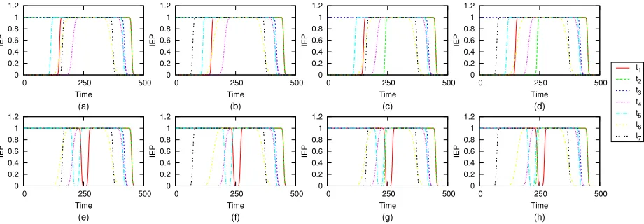
95% under the authorization A1 (i.e., I1(IEPD)), which is [217,316]as shown in Fig. 3. This result indicates that when the workflow arrives between 217 and 316 seconds, there is at least 95% of probability that when the workflow is authorized withA1, all tasks in the workflow can start execution without delay caused by the authorization constraints. Similarly, we can obtainIk(IEPD)for eachAk. Fig. 4 shows the IEP curves for all possible Ak. SAk∈AIk(IEPD) (i.e., Eq. 12) is then
the interval of the workflow’s arrival times in which there is at least 95% of probability that all tasks in the workflow can start execution without delay caused by the authorization constraints.
V. THE WORKFLOW AUTHORIZATION METHODS
Section IV-A calculates the time durations when the ex-ecutions of all tasks in a workflow will not be delayed by the authorization constraints, which is S
Ak∈AEAk(t0). The delay caused by the authorization constraints for a task is defined as the time that a ready task (a task in a workflow is ready when all of its predecessors have been completed) has to wait until the role assigned to the task becomes activated. The delay caused by the authorization constraints for a workflow (denoted by td) is defined as the total delay caused by the authorization constraints for the workflow. When a workflow arrives beyond S
Ak∈AEAk(t0), it is useful to quantitatively determinetd. Further, it is desired to develop an authorization method that can minimize td. This section strives to achieve these.
In this section, we first propose an intuitive policy of authorizing the tasks in a workflow, called the EAF (Earliest
Algorithm 1. The EAF authorization method
1 Obtain all feasible authorization solutions using
the CSP (Constraint Satisfaction Program) formulation;
2 for a ready task ti in the workflow
3 Search the set of feasible authorization
solutions to obtain a set of roles (denoted
by CA(ti)) that can be assigned to ti;
4 if all roles in CA(ti) are not activated,
5 Assign to ti a role with the earliest activation
time;
6 if there are the roles in CA(ti) that are activated,
7 A role is randomly selected and assigned to ti;
Activation First) method. Then we conduct quantitative anal-ysis about the delay caused by temporal constraints. Based on the delay analysis, we further propose a optimized method of authorizing the tasks in a workflow, called the GAA (Global Authorization-Aware) method. The GAA method is optimal in the sense that the method can minimize the delay caused by the temporal constraints. GAA is designed for the scenario where the exact execution times of the workflow tasks are known. In last subsection, we extend the GAA method to work with the stochastic workflows, where we only know the probability distributions of the tasks’ execution times.
A. The EAF authorization method
The EAF method is intuitive. Its fundamental idea is that when a task in the workflow is ready to run (i.e., all pre-decessors of the task have completed the executions), but all roles that can be assigned to the task (i.e., satisfy the authorization constraints) are not activated, a role with the earliest activation time will be assigned. The EAF method is outlined in Algorithm 1.
The workflows with different arrival times may have dif-ferent delay, td, caused by the authorization constraints for a workflow. td(τ) denotes the delay experienced by the workflow whose arrival time isτ.tdEAF(τ)denotes the delay experienced by all tasks in the workflow whose arrival time is
τ when the EAF authorization method is applied.
B. The GAA authorization method
Assume a workflow arrives at time τ. EAk(t0).next(τ) denotes the beginning of the next duration afterτ inEAk(t0). If the workflow waits for(EAk(t0).next(τ)−τ), thenAk can be used as the authorization solution of the workflow and the workflow execution can progress without further delay caused by the temporal constraints.
0 0.2 0.4 0.6 0.8 1 1.2
0 250 500
IEP Time (a) 0 0.2 0.4 0.6 0.8 1 1.2
0 250 500
IEP Time (b) 0 0.2 0.4 0.6 0.8 1 1.2
0 250 500
IEP Time (c) 0 0.2 0.4 0.6 0.8 1 1.2
0 250 500
IEP Time (d) 0 0.2 0.4 0.6 0.8 1 1.2
0 250 500
IEP Time (e) 0 0.2 0.4 0.6 0.8 1 1.2
0 250 500
IEP Time (f) 0 0.2 0.4 0.6 0.8 1 1.2
0 250 500
IEP Time (g) 0 0.2 0.4 0.6 0.8 1 1.2
0 250 500
[image:9.612.77.537.52.212.2]IEP Time (h) t1 t2 t3 t4 t5 t6 t7
Fig. 4. The IEP curves for all feasible authorizations in the case study.
whether it is EAF or GAA, checks all feasible authorization solutions to find most appropriate one.
LettdGAA(τ)denote the delay caused by the temporal con-straints for a workflow whose arrival time isτ under the GAA method. Then tdGAA(τ) equals to (EA
k(t0).next(τ)−τ). Assume that a workflow arrives at the time pointτ, and assume that it turns out that Ak is the authorization solution used for the workflow under the EAF method. We can prove that the delay caused by the temporal constraints for the workflow under the EAF method equals to (EAk(t0).next(τ)−τ), as shown in Theorem 1.
Theorem 1. If a workflow arriving at time τ is authorized using the EAF method and the outcome is that the roles are assigned to the tasks in the workflow as in the authorization solution Ak, then Eq.14 holds.
tdEAF(τ) = (EAk(t0).next(τ)−τ) (14)
Proof: If the role assigned to t0 in Ak (i.e., r(t0)) is only activated at time EAk(t0).next(τ), then t0 starts execution at EAk(t0).next(τ) under the EAF method. Con-sequently, the delay caused by the temporal constraints on
t0 is EAk(t0).next(τ)−τ, and according to the definition of EAk(t0).next(τ), all successors of t0 can start execution without further delay caused by the temporal constraints. Then
tdEAF(τ) = (EAk(t0).next(τ)−τ).
Therefore, Eq.14 holds. We call EAk(t0).next(τ) t0’s effective start time (denoted byest0).
When t0 starts at EAk(t0).next(τ), we can calculate the start time oft0’s any successorti, which is calledti’s effective start time (denoted byesti) because iftistarts at timeesti, all successors oftican start execution without being delay by the temporal constraints of the roles assigned to the successors in
Ak.esti equals est0 plus the length of the longest path from
t0 toti in the workflow.
If taskt0starts execution at timeτ00 when the role assigned to t0 inAk becomes activated, then the delay caused by the temporal constraints on t0 isτ00 −τ. Assumetk ist0’s child. Ift0 starts execution atτ00, thentk can be ready for execution
(tk’s ready time is denoted byτk) at time τ00 plus the length of the longest path fromt0totk(i.e., all its predecessors have been completed), that is, τ0
0+ (estk−est0), only subject to the availability of roler(tk).
If r(tk) is activated only at estk, then tk’s delay caused by r(tk)’s temporal constraints is estk − (τ00 + (estk −
est0))=est0−τ00, and all successors oftk can start executions without being delayed by temporal constraints. Therefore,
tdEAF(τ)can be calculated as
tdEAF(τ) = (est
0−τ00) + (τ00 −τ)
= est0−τ
= EAk(t0).next(τ)−τ
It shows Eq.14 holds.
If r(tk) is activated at time τk0 (τ 0
k < estk), then tk starts execution atτk0 in the EAF method. We can repeat the analysis similar as above only replacingt0withtk,τ withτkandest0 withestk. Similarly, we can recursively conduct the analysis for the rest of all tasks in the workflow. It can be shown that Eq.14 holds.
Besides the EAF method, other authorization method can be used to assign the roles to the tasks in a workflow. Based on Theorem 1, however, we can prove that no matter what authorization method is used to authorize the workflow, if it turns out that the workflow is authorized as in the authorization solution Ak, then the delay caused by the authorization con-straints under the authorization method will be no less than the delay when using the EAF method to assign the roles to the tasks as in Ak. This relation is stated in Theorem 2. The proof of the theorem takes the similar steps as those in Theorem 1. The difference is that when using the EAF method to authorize the tasks as Ak, a task is authorized as soon as the role assigned to the task inAk becomes activated, while under other authorization method, a task may be authorized (therefore start execution) later than the role’s activation time.
under the authorization method is no less than the delay when using the EAF method to authorize the tasks as in Ak.
Proof:Assume that a workflow arrives at timeτ. Similar to Theorem 1, we can determine esti for every task in the workflow.
If r(t0) inAk is activated at time EAk(t0).next(τ), then the minimal delay caused by the authorization constraints is
EAk(t0).next(τ)−τ, which equals to the delay generated when using the EAF method to authorizet0. Any method that authorizest0later thanEAk(t0).next(τ)will generate a delay greater than that generated by the EAF method. The theorem holds.
If r(t0) becomes activated at time τ00, but under the au-thorize method, task t0 is authorized and starts execution at a later time τ00 +δ0 (δ0 >0), then the delay caused by the authorization constraints on t0 isτ00 +δ0−τ.
Assumetkist0’s child. Ift0starts execution atτ00+δ0, then
tkcan be ready for execution at timeτk=τ00+δ0+(estk−est0). Assume τ00 +δ0 + (estk −est0) ≥ estk. Then tk can be authorized and start execution immediately and further, all successors of tk can be authorized and start execution immediately when they are ready for execution. Therefore, the minimal delay for the workflow is τ00 +δ0 −τ. Since
τ00+δ0+ (estk−est0)≥estk, we can have δ0> est0−τ00. Then the following inequality holds, which shows that the EAF method generates the minimal delay.
τ00+δ0−τ > est0−τ
= EAk(t0).next(τ)−τ
= tdEAF(τ)
Assume τ00+δ0+ (estk−est0)< estk. We can repeat the same analysis on tk as that on t0, only replacing t0 with tk,
τ withτk and est0 with estk. Similarly, we can recursively conduct the analysis for the rest of all tasks in the workflow. It can be shown that the theorem holds.
Based on Theorem 1 and 2, we can further prove that the GAA method is the optimal authorization method, as shown in Theorem 3.
Theorem 3. The GAA authorization method is optimal in the sense that under the GAA method, the delay caused by the authorization constraints for a workflow is not more than that under any other authorization method.
Proof: Given an authorization method and a workflow arriving at timeτ, assume that the method authorizes the tasks as in the authorization solution Ak. From Theorem 2, we know that the delay generated by the authorization method is no less than the delay when using the EAF method to authorize the tasks as in Ak. From Theorem 1, we know that the delay generated by the EAF method can be calculated as EAk(t0).next(τ)−τ. Therefore, the given authorization method generates a delay greater than EAk(t0).next(τ)−τ. According to the algorithm of the GAA method, the GAA method selects the authorization solutionAj that has the least
value of(EAj(t0).next(τ)−τ)from all possible authorization solutions. Therefore, the theorem holds.
C. Extending the GAA method to stochastic workflows
The previous subsections present the methods for autho-rizing the workflows in which the tasks’ execution times are exactly known. In this subsection, we extend the GAA method to authorize the worklfow whose constituent tasks have statistically distributed execution times.
When a workflow arrives at time pointτ, we apply Eq. 10 and 11 to calculate which authorization solution provides the highest value ofIEP(τ). The calculated authorization solution is then used to authorize the workflow. We call this method the MinIEP method.
In some cases, we want to maximize the opportunity that the arriving workflows can achieve the desired IEP. In or-der to achieve this, we propose the SGAA (Statistic Global Authorization-Aware) method. In SGAA, we first apply Eq. 10 and 12 to calculate the intervals in which the workflow can acquire the desiredIEPD and also record the corresponding authorization solution that can realize the IEPD.
Assume a workflow arrives at a time point τ. If τ is within one of the calculated intervals, the workflow is im-mediately authorized with the corresponding authorization solution. Otherwise, the workflow waits until the start of next nearest interval inI(IEPD)before it is authorized using the
corresponding authorization solution.
VI. SIMULATION EXPERIMENTS
We conducted the simulation experiments to evaluate the performance of the GAA method against that of the EAF method. The performance metrics evaluated in the experiments include the delay caused by the authorization constraints for a workflow (i.e.,tddefined in the first paragraph of Section V) and the response time of a workflow (denoted asrt), which is defined as the duration between the time when a first task of the workflow arrives and the time when the last tasks of the workflow is completed.
TABLE VII EXPERIMENTAL SETTINGS
Parameter Value Parameter Value
T N U M 15 M AX DG 3
EXH 5 RN U M 5
M AX RCST 3 N U M SoD 4
N U M BoD 4 P 480
T EM P 20%
we call it ahit. We record the proportion of the workflow in-stances for which the authorization decisions made by SGAA hit, which we call the hit ratio. Finally, we employ EAF to process these workflow instances and record its hit ratio. A better authorization method should have a higher hit ratio.
In the experiments, the workflow is randomly generated. Each workflow containing TNUM tasks and each task in a workflow having the maximum of M AX DG children. RNUM roles are assume to exist in the system. The tasks’ role constraints (i.e., the set of roles that a task can assume) are set in the following fashion. The simulation sets a max-imum number of roles that any task can assume in the role constraints, denoted as M AX RCST, which represents the level of restrictions imposed on the role assignment for tasks. When setting the role constraint for taskti, the number of roles that can runtiis randomly selected from [1,M AX RCST], and then that number of roles are randomly selected from the role set.
N U M SoDandN U M BoDdenote the number of tasks that are associated with SoD and BoD constraints, respectively. Duty constraints were set as follows. Each time, two tasks are randomly selected from the workflow to establish the BoD constraint between them untilN U M BoDtasks are covered. And then the same procedure is applied to establish the SoD constraints among tasks. In this process, the method presented in Section III is used to make sure that the designated duty constraints on these selected tasks can be satisfied. We assume that the tasks execution times follow an exponential distribution. The average execution time of the tasks is the
EX H time units. In order to examine the delay caused by the authorization constraints, a workflow instance is only issued after the previous instance has been completed in the experiments. Unless otherwise stated, the value of dt or rt
depicted in the figure is the value averaged over all workflow instances issued within the period of the temporal constraints, which are set below.
The temporal constraints on roles are set in the following way. For each role, a time duration is selected from a period of
Ptime units. The selected time duration occupies the specified percentage of thePtime units, which is denoted as TEMP. The starting time of the selected duration is chosen randomly from the range of [0, P×(1−T EM P)]. For example, if P=100 andTEMP=10%, the starting point is randomly selected from 0 to 90%×100.
Unless otherwise stated, the parameters are set to be the values shown in Table VII.
10 % 20 % 30 % 40 %
0 50 100 150
TEMP
td
[image:11.612.323.544.53.287.2]GAA EAF
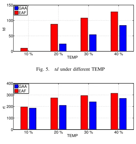
Fig. 5. tdunder different TEMP
10 % 20 % 30 % 40 %
0 100 200 300 400
TEMP
rt
[image:11.612.82.268.76.141.2]GAA EAF
Fig. 6. rtunder different TEMP
A. Temporal constraints
Fig. 5 shows the change of td as the temporal constraints (TEMP) changes. It can be seen from this figure that in all cases the GAA method achieves smaller td than EAF. For example, when TEMP is 10%, td is 0 under GAA while it is about 10 under EAF. The discrepancy becomes even bigger when TEMP increases. These results verify that the authorization method indeed matters and the GAA method is superior to the intuitive EAF method.
Fig. 6 compares rt achieved by GAA and EAF under different TEMP. It can be seen that GAA achieves the shorter
rt than EAF in all cases. This is because GAA causes less delay and therefore achieves less response time than that under EAF.
B. Arrival times of workflows
The work in this paper presents the method to determine the duration of the time for workflow arrivals within which the authorization constraints will not have negative performance impact. This shows that the arrival time of a workflow has impact on workflow performance. Fig. 7 shows the value of
[image:11.612.326.543.164.282.2]0 60 120 180 240 300 0
50 100 150
Workflow Arrival Time
td
[image:12.612.325.544.58.149.2]EAF GAA
Fig. 7. tdunder different workflow arrival times
0 60 120 180 240 300
0 100 200 300 400
Workflow Arrival Time
rt
[image:12.612.65.279.61.145.2]EAF GAA
Fig. 8. rtunder different workflow arrival times
caused under the EAF method either. This is because the time point 300 happens to be within the intersection of EAk(t0) of all feasible authorization solutions. Therefore, the system can always find an activated role for any task to enable its execution.
Fig. 8 shows that rtof the workflows with different arrival times. Again, GAA outperforms EAF in all cases. Therttrend is consistent with the tdtrend shown in Fig. 7.
C. Execution times of the workflow tasks
Obviously, increasing the execution times of the tasks in a workflow will increase the schedule length of the workflow. But do the execution times affect the authorization-related delay? Fig.9 shows the impact of the average execution time of the tasks in a workflow on the coverage of the temporal constraints (CTC), i.e.,S
Ak∈AEAk(t0). As can be seen from this figure, CTC decreases as the average execution time increases. A reasonable explanation for this is that given a set of temporal constraints, the bigger the execution time of the tasks in a workflow is, the less likely the duration of the workflow execution fits into the temporal constraints. Therefore, CTC may become shorter. This result suggests that given a set of temporal constraints, a workflow with longer tasks may be more likely to be delayed by the temporal constraints that a workflow with shorter tasks, which can be verified by the results presented in Fig. 10.
Fig. 10 demonstrates td under different average execution time of workflow tasks. Again, GAA causes less delay than EAF in all cases. It can also be observed from this figure that td increases as the average execution time of workflow tasks increases. The results coincides with the results in Fig.9. Indeed, When the execution times increases, CTC decreases. Then more workflow instances issued in the period of the temporal constraints will experience td. Consequently, td,
5 15 25 35
200 220 240 260 280 300
Average Execution Time of Workflow Tasks
[image:12.612.66.280.182.274.2]CTC
Fig. 9. rtunder different average execution times of workflow tasks
5 15 25 35
0 50 100 150
Average Execution Time of Workflow Tasks
td
EAF GAA
Fig. 10. The coverage of temporal constraints (CTC) under different average execution times of workflow tasks
which is the delay averaged over all workflow instances issued, is bigger.
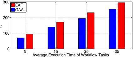
Fig. 11 showsrtgenerated by the GAA and the EAF method under different average execution time of workflow tasks. As can be observed, the GAA method generates shorter rt than EAF in all cases. This again verifies GAA causes less delay than EAF.
D. Hit ratio
In this subsection, we first generate 1000 instances of the workflow in Fig. 1 with the tasks’ execution times following the normal distribution. The values of the mean and standard deviation of the distribution for each workflow task are listed in Table VI.
Fig. 12 shows the comparison between SGAA and EAF in terms of the hit ratio. Although The hit ratio curves show the similar trend for the two method, SGAA produces much higher hit count than EAF and in some places (i.e., in the time interval of[217,316]) the hit counts of SGAA is nearly 100%. This result indicates that there are much higher proportion of authorization decisions made by SGAA that are the same as those made by GAA, compared with EAF. As can be seen
5 15 25 35
0 100 200 300
Average Execution Time of Workflow Tasks
rt
[image:12.612.327.545.185.277.2]EAF GAA
[image:12.612.329.543.612.705.2]0 0.2 0.4 0.6 0.8 1
0 80 160 240 320 400 480
Hit Ratio
Time
[image:13.612.73.275.53.194.2]SGAA EAF
Fig. 12. Comparing the hit ratio between SGAA and EAF
0 0.2 0.4 0.6 0.8 1 1.2
10% 20% 30% 40%
Mean Hit Ratio
TEMP
SGAA EAF
Fig. 13. The hit ratio comparison under differentT EM P
from the figure, the hit count of EAF becomes unstable in some places (the dip in the EAF curve) and lower than other places. This may be because of the local optimum nature of the EAF method. Namely, some authorization solutions may enter the wrong “branches” of the workflow (e.g.,t1as shown in our experimental records). In contrast, the performance of SGAA is almost always stable. These experimental results also show that IEP and the optimal interval are effective metrics for measuring the impacts of authorization constraints on workflow executions.
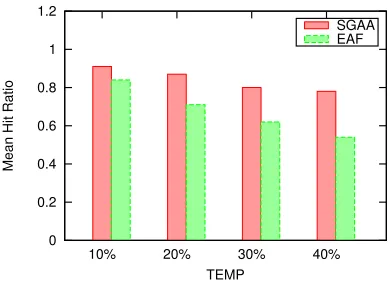
We then change the temporal constraints using the way presented at the beginning of this section. Fig. 13 shows the mean hit ratio achieved by SGAA and EAF under different
T EM P. It can be seen again that SGAA achieves the higher hit ratio than EAF in all cases. This is because SGAA takes into account the situation of the entire workflow and seek for global optimization and therefore is able to make better decisions than EAF.
VII. CONCLUSIONS
This paper investigates the issue of feasibility checking for authorization constraints deployed in workflow management systems. In this paper, the feasibility checking problem is modelled as a constraint satisfaction problem. Further, this paper presents the method to determine the time durations when the deployed temporal constraints do not have negative impact on performance of workflow executions. Moreover,
an optimal method is proposed to authorize a workflow, so that the delay caused by the authorization constraints for the workflow executions is minimized. The proposed analysis methods are further extended for the stochastic workflows. The simulation experiments show that the effectiveness of the proposed authorization methods.
VIII. ACKNOWLEDGEMENT
The preliminary version of this work has been published in the 20th International Conference on High Performance Computing (HiPC-2013) [28]. This work is partially supported by the Priority Academic Program Development of Jiangsu Higer Education Institutions (PAPD), Jiangsu Collaborative Innovation Center on Atmospheric Environment and Equip-ment Technology (CICAEET), the Natural Science Foundation of China (NSFC) under Grant Nos. 61472370 and 61672469, and the open project of State Key Laboratory of virtual reality technology and system under Grant No. BUAA-VR-16KF-07.
REFERENCES
[1] D. Chakraborty, V. Mankar, and A. Nanavati, “Enabling runtime adapta-tion ofworkflows to external events in enterprise environments,” inWeb Services, 2007. ICWS 2007. IEEE International Conference on, july 2007, pp. 1112 –1119.
[2] E. Deelman, D. Gannon, M. Shields, and I. Taylor,
“Workflows and e-science: An overview of workflow system
features and capabilities,” Future Generation Computer Systems,
vol. 25, no. 5, pp. 528 – 540, 2009. [Online]. Available:
http://www.sciencedirect.com/science/article/pii/S0167739X08000861 [3] A. Sfrent and F. Pop, “Asymptotic scheduling for many task
computing in big data platforms,” Information Sciences, vol. 319, pp. 71 – 91, 2015, energy Efficient Data, Services and Memory Management in Big Data Information Systems. [Online]. Available: http://www.sciencedirect.com/science/article/pii/S0020025515002182 [4] M.-A. Vasile, F. Pop, R.-I. Tutueanu, V. Cristea, and J. Koodziej,
“Resource-aware hybrid scheduling algorithm in heterogeneous
distributed computing,” Future Generation Computer Systems,
vol. 51, pp. 61 – 71, 2015, special Section: A Note
on New Trends in Data-Aware Scheduling and Resource
Provisioning in Modern {HPC} Systems. [Online]. Available:
http://www.sciencedirect.com/science/article/pii/S0167739X14002532 [5] G.-J. Ahn and R. Sandhu, “Role-based authorization constraints
speci-fication,”ACM Trans. Inf. Syst. Secur., vol. 3, no. 4, pp. 207–226, Nov. 2000. [Online]. Available: http://doi.acm.org/10.1145/382912.382913 [6] J. B. D. Joshi, E. Bertino, U. Latif, and A. Ghafoor, “A generalized
temporal role-based access control model,”IEEE Trans. on Knowl. and Data Eng., vol. 17, no. 1, pp. 4–23, Jan. 2005. [Online]. Available: http://dx.doi.org/10.1109/TKDE.2005.1
[7] D. Zou, L. He, H. Jin, and X. Chen, “Crbac: Imposing multi-grained constraints on the rbac model in the multi-application
environment,” Journal of Network and Computer Applications,
vol. 32, no. 2, pp. 402 – 411, 2009. [Online]. Available:
http://www.sciencedirect.com/science/article/pii/S1084804508000520 [8] V. Atluri and W. kuang Huang, “A petri net based safety analysis of
workflow authorization models,” 1999.
[9] M. Stuit, H. Wortmann, N. Szirbik, and J. Roodenburg,
“Multi-view interaction modelling of human collaboration processes:
A business process study of head and neck cancer care
in a dutch academic hospital,” J. of Biomedical Informatics,
vol. 44, no. 6, pp. 1039–1055, Dec. 2011. [Online]. Available: http://dx.doi.org/10.1016/j.jbi.2011.08.007
[image:13.612.77.272.223.365.2][11] J. Y. Choi and S. Reveliotis, “A generalized stochastic petri net model for performance analysis and control of capacitated reentrant lines,” Robotics and Automation, IEEE Transactions on, vol. 19, no. 3, pp. 474 – 480, june 2003.
[12] D. R. dos Santos, S. E. Ponta, and S. Ranise, “Modular synthesis of enforcement mechanisms for the workflow satisfiability problem: Scalability and reusability,” in Proceedings of the 21st ACM on Symposium on Access Control Models and Technologies, ser. SACMAT ’16. New York, NY, USA: ACM, 2016, pp. 89–99. [Online]. Available: http://doi.acm.org/10.1145/2914642.2914649
[13] C. Bertolissi, D. R. dos Santos, and S. Ranise, “Automated synthesis of run-time monitors to enforce authorization policies in business processes,” inProceedings of the 10th ACM Symposium on Information, Computer and Communications Security, ser. ASIA CCS ’15. New York, NY, USA: ACM, 2015, pp. 297–308. [Online]. Available: http://doi.acm.org/10.1145/2714576.2714633
[14] J. Crampton, G. Gutin, and D. Karapetyan, “Valued workflow satisfiability problem,” in Proceedings of the 20th ACM Symposium on Access Control Models and Technologies, ser. SACMAT ’15. New York, NY, USA: ACM, 2015, pp. 3–13. [Online]. Available: http://doi.acm.org/10.1145/2752952.2752961
[15] J. Crampton, “A reference monitor for workflow systems with
constrained task execution,” in Proceedings of the tenth ACM
symposium on Access control models and technologies, ser. SACMAT ’05. New York, NY, USA: ACM, 2005, pp. 38–47. [Online]. Available: http://doi.acm.org/10.1145/1063979.1063986
[16] Q. Wang and N. Li, “Satisfiability and resiliency in workflow authorization systems,” ACM Trans. Inf. Syst. Secur., vol. 13,
no. 4, pp. 40:1–40:35, Dec. 2010. [Online]. Available:
http://doi.acm.org/10.1145/1880022.1880034
[17] Y. Lu, L. Zhang, and J. Sun, “Using colored petri nets to model and analyze workflow with separation of duty constraints,” The International Journal of Advanced Manufacturing Technology, vol. 40, pp. 179–192, 2009, 10.1007/s00170-007-1316-1. [Online]. Available: http://dx.doi.org/10.1007/s00170-007-1316-1
[18] L. He, C. Huang, K. Duan, K. Li, H. Chen, J. Sun,
and S. A. Jarvis, “Modeling and analyzing the impact of
authorization on workflow executions,” Future Gener. Comput.
Syst., vol. 28, no. 8, pp. 1177–1193, Oct. 2012. [Online]. Available: http://dx.doi.org/10.1016/j.future.2012.03.003
[19] L. He, N. Chaudhary, S. Jarvis, and K. Li, “Allocating resources for workflows running under authorization control,” in Grid Computing (GRID), 2012 ACM/IEEE 13th International Conference on, 2012, pp. 58–65.
[20] K. Jensen, L. M. Kristensen, and L. Wells, “Coloured petri nets and cpn tools for modelling and validation of concurrent systems,”Int. J. Softw. Tools Technol. Transf., vol. 9, no. 3, pp. 213–254, May 2007. [Online]. Available: http://dx.doi.org/10.1007/s10009-007-0038-x
[21] S. C. Brailsford, C. N. Potts, and B. M. Smith,
“Constraint satisfaction problems: Algorithms and
applica-tions,” European Journal of Operational Research, vol.
119, no. 3, pp. 557 – 581, 1999. [Online]. Available:
http://www.sciencedirect.com/science/article/pii/S0377221798003646 [22] R. H. M¨ohring, A. S. Schulz, and M. Uetz, “Approximation in
stochastic scheduling: The power of lp-based priority policies,” J. ACM, vol. 46, no. 6, pp. 924–942, Nov. 1999. [Online]. Available: http://doi.acm.org/10.1145/331524.331530
[23] X. Tang, K. Li, G. Liao, K. Fang, and F. Wu, “A stochastic scheduling algorithm for precedence constrained tasks on grid,” Future Gener. Comput. Syst., vol. 27, no. 8, pp. 1083–1091, Oct. 2011. [Online]. Available: http://dx.doi.org/10.1016/j.future.2011.04.007
[24] J. Gu, X. Gu, and M. Gu, “A novel parallel quantum genetic algorithm for stochastic job shop scheduling.”Journal of Mathematical Analysis and Applications, vol. 355, no. 1, pp. 63–81, 2009.
[25] S. C. Sarin, B. Nagarajan, and L. Liao, Stochastic scheduling. Expectation-variance analysis of a schedule. Cambridge: Cambridge University Press, 2010.
[26] V. J. Duko Leti, “The distribution of time for clark flow and risk assessment for the activities of pert network structure,”The Yugoslav Journal of Operations Research, no. 37, pp. 195–207, 2009. [Online]. Available: http://eudml.org/doc/261518
[27] C. E. Clark, “The Greatest of a Finite Set of Random Variables,” Operations Research, vol. 9, pp. 145–162, 1961.