warwick.ac.uk/lib-publications
Original citation:
Deng, Yansha, Noel, Adam, Guo, Weisi, Nallanathan, Arumugam and Elkashlan, Maged.
(2017) Analyzing large-scale multiuser molecular communication via 3D stochastic geometry.
IEEE Transactions on Molecular, Biological and Multi-Scale Communications.
Permanent WRAP URL:
http://wrap.warwick.ac.uk/91752
Copyright and reuse:
The Warwick Research Archive Portal (WRAP) makes this work by researchers of the
University of Warwick available open access under the following conditions. Copyright ©
and all moral rights to the version of the paper presented here belong to the individual
author(s) and/or other copyright owners. To the extent reasonable and practicable the
material made available in WRAP has been checked for eligibility before being made
available.
Copies of full items can be used for personal research or study, educational, or not-for profit
purposes without prior permission or charge. Provided that the authors, title and full
bibliographic details are credited, a hyperlink and/or URL is given for the original metadata
page and the content is not changed in any way.
Publisher’s statement:
“© 2017 IEEE. Personal use of this material is permitted. Permission from IEEE must be
obtained for all other uses, in any current or future media, including reprinting
/republishing this material for advertising or promotional purposes, creating new collective
works, for resale or redistribution to servers or lists, or reuse of any copyrighted component
of this work in other works.”
A note on versions:
The version presented here may differ from the published version or, version of record, if
you wish to cite this item you are advised to consult the publisher’s version. Please see the
‘permanent WRAP URL’ above for details on accessing the published version and note that
access may require a subscription.
arXiv:1704.06929v2 [cs.IT] 10 May 2017
Analyzing Large-Scale Multiuser Molecular
Communication via 3D Stochastic Geometry
Yansha Deng,
Member, IEEE,
Adam Noel,
Member, IEEE,
Weisi Guo,
Member, IEEE,
Arumugam Nallanathan,
Fellow, IEEE,
and Maged Elkashlan,
Member, IEEE
.
Abstract—Information delivery using chemical molecules is an integral part of biology at multiple distance scales and has attracted recent interest in bioengineering and communication theory. Potential applications include cooperative networks with a large number of simple devices that could be randomly located (e.g., due to mobility). This paper presents the first tractable analytical model for the collective signal strength due to randomly-placed transmitters in a three-dimensional (3D) large-scale molec-ular communication system, either with or without degradation in the propagation environment. Transmitter locations in an un-bounded and homogeneous fluid are modelled as a homogeneous Poisson point process. By applying stochastic geometry, analytical expressions are derived for the expected number of molecules absorbed by a fully-absorbing receiver or observed by a passive receiver. The bit error probability is derived under ON/OFF keying and either a constant or adaptive decision threshold. Results reveal that the combined signal strength increases propor-tionately with the transmitter density, and the minimum bit error probability can be improved by introducing molecule degradation. Furthermore, the analysis of the system can be generalized to other receiver designs and other performance characteristics in large-scale molecular communication systems.
Index terms— Large-scale molecular communication
sys-tem, absorbing receiver, passive receiver, 3D stochastic geom-etry.
I. INTRODUCTION
Molecular communication via diffusion has attracted sig-nificant bioengineering and communication engineering re-search interest in recent years [1]. Messages are delivered via molecules undergoing random walks [2], which is a prevalent phenomenon in biological systems and between organisms [3] across multiple distance scales, offering transmit energy and signal propagation advantages over wave-based commu-nications [4, 5]. More importantly, when compared to elec-tromagnetic wave-based communication systems, molecular communication can be advantageous at very small dimensions or in specific environments, such as in salt water or human bodies.
Y. Deng and A. Nallanathan are with Department of Informatics, King’s College London, London, WC2R 2LS, UK (email:{yansha.deng, aru-mugam.nallanathan}@kcl.ac.uk).
A. Noel is with the School of Electrical Engineering and Computer Science, University of Ottawa, Ottawa, ON, K1N 6N5, Canada (email: [email protected]).
Weisi Guo is with School of Engineering, University of Warwick, West Midlands, CV4 7AL, UK (email: [email protected]).
M. Elkashlan is with Queen Mary University of London, London, E1 4NS, UK (email: [email protected]).
Fundamentally, molecular communications involves modu-lating information on the physical properties (e.g., number, type, emission time) of a single molecule or group of molecules (such as pheromones, DNA, protein). When modulating the number of molecules, each messenger node will transmit information-bearing molecules via chemical pulses. According to the theory of Brownian motion, the average displacement of each molecule is proportional to its diffusion time and the diffusion coefficient, however, the instantaneous displacement of each molecule differs and is usually described by the Normal distribution [6]. As such, a molecule emitted in a previous bit interval may arrive at the receiver during the current interval, thereby confusing the signal detection at the receiver with intersymbol interference (ISI).
Existing works have largely focused on modeling the signal strength of a point-to-point communication channel by taking into account the self-interference that arises from previous symbols (i.e., ISI) at a passive receiver [7], at a fully absorbing receiver [8], and at a reversible adsorption receiver [9]. Efforts to mitigate ISI include transmitting using two different types of molecules in consecutive bit intervals [10], and designing ISI-free codes [11].
Recent advances in bio-nanotechnology bring new opportuni-ties for enabling molecular communication in new applications, such as drug delivery, environmental monitoring, and pollution control. One application example is that swarms of nano-robots could track specific targets, such as tumour cells, to perform operations such as targeted drug delivery [12]. In such a scenario, each nano-robot may receive the signal transmitted from multiple nano-robots. Thus, how to establish energy efficient and tether-less communication becomes an important research problem [13].
where the probability density function (PDF) of the received power spectral density at a point receiver was derived based on the assumption of white Gaussian transmit signals. The analysis in [16] considered multiuser emission within a single transmission interval, and the presented results were Monte Carlo simulations.
From the perspective of receiver design, many works have focused on the passive receiver, which can observe and count the number of molecules inside the receiver without interfering with the molecules [7, 14, 16]. In nature, receivers commonly remove information molecules from the environment once they bind to a receptor. An ideal model is the fully absorbing re-ceiver, which absorbs all the molecules hitting its surface [8, 9]. Unfortunately, no work has studied the channel characteristics and the received signal at a fully absorbing receiver in a large-scale molecular communication system, nor compared it with that at a passive receiver.
In this paper, we aim to provide an analytical model and bit error probability for the collective signal at the passive receiver and the fully absorbing receiver due to a swarm of active mobile point transmitters that simultaneously emit the same bit sequence. We extend our previous work in [17] by deriving the bit error probability of a constant threshold detector at both receivers under fixed threshold-based demodulation, and applying decision feedback detection (DFD) for performance improvement. Our new analysis takes into account the molecule degradation during diffusion based on the following three facts: 1) molecules are unlikely to persist for all time, and may be degraded by chemical reactions in a biological environment; 2) the constant transmitter density over unbounded space assumed in our analytical model implies that there is an infinite number of transmitters and that ISI increasingly accumulates, which isn’t practical; 3) the molecule degradation will help to reduce the ISI and improve the probability of error.
The analytical results are obtained via the powerful tools of stochastic geometry in 3D space, which can characterize the average behavior over many spatial realizations of a net-work where the transmitter nodes are placed according to some probability distribution [18]. Just as we can analyze the network performance of a random field of transmitters in conventional wireless networks, we can also apply a similar rationale for analyzing the receiver performance due to a swarm of molecular transceivers. However, unlike [19, 20], where the network performance is analyzed based on the distribution of the received signal-to-interference-plus-noise ratio (SINR) at a point receiver in 2D space, we seek the mean and distribution of the number of received molecules at a spherical receiver due to all transmitters in 3D space. By doing so, simple and tractable results can be obtained to reveal the key dependency of the molecular communication system performance metrics with respect to the system parameters. This work and [17] are distinct from related work in [16], which focused on the statistics of the received signal at any point location. Our contributions can be summarized as follows:
1) Using stochastic geometry, we model the collective signal
at a receiver in a 3D large-scale molecular commu-nication system with or without molecule degradation, where the receiver is either passive or fully absorbing. To examine the impact of the signal from the nearest transmitter relative to the aggregate signal, we also derive the signals from the nearest transmitter and the other transmitters.
2) We derive a general expression for the expected net number of molecules observed at both types of receivers during any time interval. In order to gain insights about the impact of the transmitter density, the diffusion coeffi-cient, and the receiver radius on the collective signal, we simplify the general expression to a closed-form
expression for the expected net number of molecules absorbed at the fully absorbing receiver under molecule degradation.
3) We derive a general expression for the bit error prob-ability at the passive or absorbing receiver in the pro-posed system with or without molecule degradation under ON/OFF keying. A simple detector requiring one sample per bit interval is considered as a preliminary design for the proposed large-scale system. Importantly, this general expression for the bit error probability can also be applied for other types of receivers by substituting the corresponding channel response.
4) We focus on Monte Carlo simulation approaches to verify our analytical results, and we also compare Monte Carlo simulation to particle-based simulation of the large-scale molecular communication system. It is shown that the expected number of molecules observed at both types of receivers increases linearly with increasing transmitter density. We also show that the minimum bit error prob-ability of both receivers can be improved by introducing molecule degradation.
The rest of this paper is organized as follows. In Section II, we introduce the system model. In Section III, we present the channel impulse response of information molecules in the large-scale molecular communication system. In Section IV, we derive the exact and asymptotic net number of absorbed molecules expected at the surface of the absorbing receiver, and the exact number of molecules observed inside the passive receiver in the large-scale molecular communication system. In Section V, we derive the bit error probability of the proposed system with a simple detector requiring one sample per bit. In Section VI, we present the numerical and simulation results. In Section VII, we conclude the contributions of this paper.
II. SYSTEMMODEL
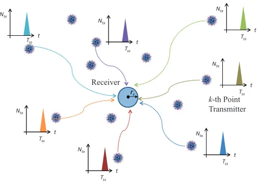
In Fig. 1, we consider a 3D diffusion-based molecular com-munication system with a single receiver located at the origin under joint transmission by a swarm of point transmitters, which are spatially distributed outside the receiver inR3/VΩrr
Receiver
k-th Point Transmitter
T
ss
t N
tx
Tss
t Ntx
T
ss
t N
tx
Tss
t Ntx
Tss
t Ntx
Tss
t Ntx
Tss
t Ntx
[image:4.612.46.298.54.233.2]rr
Fig. 1. Illustration of a receiver receiving molecular pulse signals from point transmitters at different distances.
process (HPPP)1Φ
awith densityλa, whereVΩrr is the volume
of receiverΩrr with VΩrr = 4πr 3 r
3. HPPP has been widely used to model wireless sensor networks [19], homogeneous and heterogeneous cellular networks [18], and has also been applied to model bacterial colonies in [21] and the interference sources in a molecular communication system [16]. We note that we focus on an unbounded fluid environment with uniform diffusion and no flow currents to provide a baseline for the design of more complicated scenarios in future works.
We consider a spherical receiver that is either passive [4, 22] or fully absorbing [23]. The fully absorbing receiver is covered with selective independent receptors, which are only sensitive to a single type of information molecule. Similar to [9, 23], we assume that there is no physical limitation on the number of receptors on the surface of the receiver, which is an appropriate assumption for a system with a sufficiently large number of receptors or small number of absorbed molecules. Any information molecule that diffuses into the sphere is absorbed by a receptor and counted for information demodulation. The passive receiver is covered with a transparent membrane that is permeable to the information molecules passing by, and the number of information molecules inside the receiver can be counted for information demodulation as in [14].
Even though this work considers a molecular communica-tion system with a single receiver, it provides fundamental insights that can be applied to consider systems with multiple transceivers in future work. For example, in the case of multiple passive receivers following HPPP, the expected number of molecules inside any passive receiver with the same radius will be equivalent due to the Slivnyak-Mecke’s theorem [24]. In other words, the presence of multiple passive receivers will not influence the observations at each passive receiver, due to its transparent membrane. This is also consistent with
1This model is also valid for spherical transmitters with transparent
mem-branes, where the locations of the point process are the molecule emission points.
the stochastic geometry work on cellular networks, where the average ergodic rate of an arbitrary random mobile user is expressed using a single expression [20]. However, for the case of multiple absorbing receivers, the numbers of molecules absorbed by each absorbing receiver is not independent; in other words, the presence or absence of an absorbing receiver influences the numbers of molecules absorbed by other absorb-ing receivers. For a system of absorbabsorb-ing receivers, the average observation will be harder to characterize, but understanding the single receiver system is still the first step.
A molecular communication system typically includes five processes: emission, propagation, reception, modulation, and demodulation, which are presented in detail in the following subsections for the absorbing receiver and the passive receiver, respectively.
A. Emission&Modulation
Applying ON/OFF keying as in [9, 23], each transmitter delivers molecular signal pulses with Ntx type S information
molecules to the receiver at the start of each bit interval to represent transmit bit-1, and emits zero molecules to deliver bit-0. Here, a global clock is assumed at each transmitter such that the molecule emissions at all the transmitters are synchronized with the same bit sequences2, and can only occur
at the start of a bit interval as in [16]. Asynchronous emission can be evaluated similarly to synchronous emission by allowing transmitters to release molecules at the start of intervals that are much smaller than the bit interval, and scaling the transmitter density accordingly.
1) Absorbing Receiver: In the absorbing receiver scenario, we assume spherical symmetry, where the transmitter is effec-tivelya point on the spherical shell with radiusr0away from the
center of receiver and the molecules are released from random points over the shell att= 0; the actual angle to the transmitter when a molecule hits the receiver is irrelevant. Thus, we define the initial condition as [25, Eq. (3.61)]
CFA(r, t
→0|r0) = 1
4πr02
δ(r−r0), (1)
whereCFA(r, t→0|r
0)is the molecule distribution function
at timet→0and distancer with initial distancer0 .
2) Passive receiver: In the passive receiver scenario, we assume an asymmetric spherical model, which accounts for the actual angle of the molecule inside the passive receiver. The information particles are injected into the fluid environment by a transmitter located at−→r away from the center of the passive receiver [6].
B. Diffusion Under Molecule Degradation
The diffusion of molecules in the propagation process fol-lows random Brownian motion. With a sufficiently low
con-2 One application is that nanomachines could send the same molecular
centration of information molecules in the fluid environment, the collisions between these molecules can be ignored and the molecules propagate independently with constant diffusion coefficient3 D . This concentration changes over time due to diffusion as described by Fick’s second law, and determines the spatial and temporal variation of non-uniform distributions of particles [6, Ch.2].
To reduce the ISI, we introduce molecule degradation that can occur at any time via a chemical reaction mechanism in the form of [22, 27, 28]
S→kdP, (2)
where kd is the degradation rate in s−1, and P is another
type of molecule that cannot be recognized by either type of receiver. The degradation ratekd relates to the half-life (Λ1/2)
of messenger molecules viakd=Λln 21/2, andkd= 0corresponds to the no degradation case.
C. Reception
1) Absorbing Receiver: Any information molecules that hit the absorbing receiver will be captured for information demodulation. This reception process at the fully absorbing receiver can be described as [25]
D∂ C
FA(r, t|r
0)
∂r
r=r+r
=kCFA(r
r, t|r0), k→ ∞ (3)
wherekis the absorption rate (in length×time−1).
2) Passive receiver: With a transparent membrane at the passive receiver, the information molecules can bypass the surface of the passive receiver freely, and molecules within the receiver can be counted at any time [6].
D. Demodulation
For equivalent comparison, the number of molecules ab-sorbed by the surface of the absorbing receiver and the number of observed molecules inside the passive receiver at the end of each bit interval are collected for information demodulation. More details of the demodulation at each type of receiver are described as follows.
1) Demodulation criterion at the absorbing receiver: With spherical symmetry, we only need to focus on the number of molecules absorbed by the surface of the receiverr=rr. We
consider an absorbing receiver that is capable of counting the net number of molecules absorbed by the surface of the receiver at as in [9] by subtracting the number of absorbed molecules at the end of the previous bit interval from that at the end of the current bit interval. The net number of molecules absorbed over thejth bit intervalNFA
net[j]is demodulated as the received
signal of the jth bit (NRx[j] = NFA
net[j]). This is because
for the single bit transmission at t = 0, as time increases, the number of absorbed molecules increases, which results in
3The diffusion coefficient can be obtained via experiment or estimated via
the Stokes-Einstein equation for spherical molecules [26, Ch. 5]
increasing ISI, whereas the average net number of absorbed molecules in a given bit intervalTb becomes a constant value
asTbgoes to infinity in a large-scale molecular communication
system as shown in Section IV.
2) Demodulation criterion at the passive receiver: With a transparent membrane, the passive receiver is assumed to be capable of counting the number of molecules currently inside the passive receiver at the end of the jth bit interval NcurPA[j]
for information demodulation (NRx[j] = NcurPA[j]). This is
because the current number of observed molecules inside the receiver can remain at a comparable value for a long time in the large-scale molecular communication system as will be shown in Fig. 3 in Section VI. For this reason, we only use a simple detector design with one sample collected at the end of each bit interval rather than multiple samples in each bit interval.
3) Demodulation schemes at both receivers: We first con-sider a fixed threshold-based demodulation with the same decision thresholdNth for all bits at both types of receivers,
where the receiver demodulates the received signal as bit-1 if NRx[j]≥N
th, and demodulates the received signal as bit-0 if
NRx[j]< N
th. In the fixed threshold-based demodulation, the
received molecules NRx[j] will accumulate as more bits are
transmitted and molecules arrive from more distant transmitters, and inevitably impair the system reliability as ISI.
To remove this accumulation, we then consider the demodu-lation scheme using a DFD [29] with the decision thresholdNth
at both types of receivers in Section VI, based on the subtrac-tion betweenNRxin the current bit and that in the previous bit.
More specifically, the receiver demodulates the received signal as bit-1 if {NRx[j]−NRx[j−1]} ≥N
th, and demodulates
the received signal as bit-0 if{NRx[j]−NRx[j−1]}< N
th.
III. CHANNELIMPULSERESPONSE
In this section, we present the channel impulse responses at the absorbing receiver and at the passive receiver in the large-scale molecular communication system due to the single bit-1 transmission at each point transmitter.
A. Absorbing Receiver
1) Point-to-point system: We first provide the background for the receiver observation of a single point transmitter located distancer0 away from the center of the absorbing receiver. To
do so, we calculate the rate of absorption at the surface of the absorbing receiver due to the transmitter at distancer0 via [25,
Eq. (3.106)]
K(t|r0) = 4πr2rD
∂CFA(r, t|r
0)
∂r
r=rr
, (6)
where the molecule distribution function
CFA(r, t |r0) =
1 4πrr0
1
√
4πDt
e−(r−r0 ) 2 4Dt −e−
(r+r0−2rr)2 4Dt
,
(7)
Substituting (7) into (6), the first hitting probability is derived as
K(t|r0) = rr
r0
1
√
4πDt r0−rr
t e
−(r0−rr)2
4Dt . (4)
Taking into account molecule degradation, the fraction of molecules absorbed by the receiver due to a transmitter at distance r0 during any sampling interval [t, t+Tss] with a
single impulse pulse occurring att= 0 reduces to FFA( Ωrr, t, t+Tss|r0)
=FFA( Ωrr,0, t+Tss|r0)−FFA( Ωrr,0, t|r0), (5)
where
FFA( Ωrr,0, t|r0) =
Z t
0
K(t|r0)e−kdtdt
=rr
r0
exp −
r
kd
D (r0−rr)
!
−2rrr
0
exp −
r
kd
D (r0−rr)
!
"
erf
r0−rr √
4Dt −
p
kdt
+ exp 2
r
kd
D (r0−rr)
!
erf
r0−rr √
4Dt +
p
kdt
−1
+ 1
. (6)
We note that (6) is derived following the method for the the point-to-point system in [27, Eq. (12)]. We see that increasing kddecreases the fraction of molecules absorbed by the
absorb-ing receiver.
Without molecule degradation (kd = 0),FFA( Ωrr,0, t|r0)
simplifies to [23, Eq. (32)]
FFA( Ω
rr,0, t|r0) =
rr
r0
erfcnr√0−rr
4Dt
o
. (7)
2) Large-scale system: In our proposed large-scale system, the center of an absorbing receiver is fixed at the origin of a 3D fluid environment.
Using the Slivnyak-Mecke’s theorem [24], the fraction of absorbed molecules at the receiver during any sampling interval
[t, t+Tss]due to anarbitrarypoint transmitterxat the location
x emitting a single pulse at t = 0 FFA( Ω
rr, t, t+Tss| kxk)
can be obtained via (6), where kxk is the distance between the point transmitter and the center of the receiver where the transmitters follow a HPPP.
Recalling that the propagation of each molecule is indepen-dent, the cumulative fraction FFA
all of absorbed molecules at
the receiver during any sampling interval[t, t+Tss]due to all
active point transmitters emitting a single pulse at t = 0can be formulated as
FallFA(Ωrr, t, t+Tss) =
X
x∈Φa
FFA( Ωrr, t, t+Tss| kxk), (8)
whereFFA( Ωrr, t, t+Tss| kxk)can be obtained from (6).
The expected net number of molecules absorbed by the receiver during any sampling interval [t, t +Tss] due to all
of the active point transmitters emitting a single pulse att= 0
can be calculated as
ENallFA(Ωrr, t, t+Tss) =NtxE
n
FallFA(Ωrr, t, t+Tss)
o
, (9)
where NFA
all (Ωrr, t, t+Tss) is the net number of absorbed
molecules, andFFA
all (Ωrr, t, t+Tss)is given in (8).
It is well known that the distance between the transmitter and the receiver in molecular communication is the main contributor to the signal strength. In the absence of flow, the nearest transmitter will provide the strongest signal for the receiver. In order to examine the impact of the signal from the nearest transmitter on the received signal in the large-scale molecular communication system, we present the expected number of absorbed molecules at this receiver during any sampling interval [t, t+Tss] due to a single pulse emission
by the nearesttransmitter as EFAu =E
n
FFA( Ωrr, t, t+Tss| kx∗k)
o
, (10)
wherekx∗kdenotes the distance between the receiver and the nearest transmitter,
x∗= arg min x∈Φa
kxk, (11)
x∗ denotes the nearest point transmitter for the receiver, and
Φa denotes the set of active transmitters’ positions.
To examine the impact of the aggregate signal from the remaining transmitters, we present the expected number of absorbed molecules at this receiver during any sampling in-terval [t, t+Tss] due to single pulse emissions by the other
transmitters as
EFAo =E
( X
x∈Φa/x∗
FFA( Ω
rr, t, t+Tss| kxk)
)
, (12)
whereFFA( Ω
rr, t, t+Tss| kxk)is given in (6).
B. Passive Receiver
1) Point-to-point system: In a point-to-point molecular com-munication system with a single point transmitter located at−→r relative to the center of a passive receiver with radius rr, the
local point concentration at the center of the passive receiver at time t due to a single pulse emission by the transmitter occurring att= 0is given as [30, Eq. (4.28)]
C( Ωrr, t| −→r) =
1
(4πDt)3/2exp
−|−→r|
2
4Dt
, (13)
where−→r = [x, y, z], and[x, y, z]are the coordinates along the three axes.
The fraction of molecules observed inside the passive re-ceiver with volumeVΩrr at timetis denoted as
FPS( Ω
rr, t| |−→r|) =
Z
Ωrr
In most molecular communication literature considering a passive receiver, the uniform concentration assumption inside the passive receiver is applied, which immediately results in the fraction of observed molecules inside the passive receiver as
FPS( Ωrr, t| |−→r|))≈C( Ωrr, t| |−→r|)VΩrr, (15)
however, this result relies on the receiver being sufficiently far from the transmitter (see [31]), which wecannotguarantee here since the transmitters are placed randomly.
With the actualnon-uniformconcentration inside the passive receiver, the fraction of observed molecules inside the passive receiver is calculated as
FPS( Ωrr, t| |−→r|) = rr
Z
0
2π
Z
0 π
Z
0
C( Ωrr, t| −→r)r2sinθdθdφdr.
(16)
The molecule degradation introduces a decaying exponential term as in [22, Eq. (10)]. Therefore, according to (16) and Theorem 2 in [31], the fraction FPS of molecules observed
inside the passive receiver at time t due to a single pulse emission by a transmitter at r0 away from the center of a
passive receiver with radiusrr at timet= 0is derived as
FPS( Ω
rr, t|r0) =e−kdt
"
1 2
h
erfrr−r0 2√Dt
+ erfrr+r0 2√Dt
i
+
√
Dt
√
πr0
h
exp−(rr+r0)
2
4Dt
−exp−(r0−rr)
2
4Dt
i#
.
(17)
We see from (17) that increasingkd decreases the fraction of
molecules observed at the passive receiver.
2) Large-scale system: In the large-scale molecular commu-nication system with a passive receiver centered at the origin, the fraction FPS of molecules observed inside the passive
receiver at timeTssdue to anarbitrarypoint transmitterxat the
location x emitting a single pulse at t= 0, FPS( Ω
rr, t| kxk)
can be obtained using (17).
Due to the independent propagation of each molecule, the expected number of molecules observed inside the receiver at timeTss due to a single pulse emission byall transmitters at
t= 0is given as
ENallPS(Ωrr, Tss) =NtxE
n
FPS( Ωrr, Tss| kx∗k)
o
| {z }
EPS u
+NtxE
( X
x∈Φa/x∗
FPS( Ω
rr, Tss| kxk)
)
| {z }
EPS o
, (18)
whereFPS( Ω
rr, Tss| kxk) is obtained using (17), EPSu is the
expected number of molecules observed inside the receiver at timeTssdue to the nearest transmitter, andEPSo is the expected
number of molecules observed inside the receiver at timeTss
due to the other transmitters.
IV. RECEIVEROBSERVATIONS
In this section, we first derive the distance distribution be-tween the receiver and the nearest point transmitter. Throughout this section, we focus on the receiver observations at the receivers due to a single emission at each point transmitter att = 0. To understand the impact of individual TXs relative to the aggregate signal, we derive exact expressions for the ex-pected number of molecules observed at the receiver due to the nearest point transmitter and that due to the other transmitters. We then present exact expressions for the expected number of molecules observed at the receiver due to all transmitters.
A. Distance Distribution
Unlike the stochastic geometry modelling of wireless net-works, where the transmitters are randomly located in un-bounded space, we impose that the point transmitters in a molecular communication system can only be distributed out-side the surface of the spherical receiver. Taking into account the minimum distance rr between point transmitters and the
receiver center, we derive the PDF of the shortest distance between a point transmitter and the receiver with radius rr
in the following proposition.
Proposition 1. The PDF of the shortest distance between any point transmitter and the receiver with radiusrr in 3D space
is
fkx∗k(x) = 4λaπx2e−λa(
4 3πx
3−4 3πrr
3)
. (19)
Proof. See Appendix A.
Based on the proof of Proposition 1, we also derive the PDF of the shortest distance between any point transmitter and the receiver in 2D space in the following lemma.
Corollary 1. The PDF of the shortest distance between any point transmitter and the receiver in 2D space is given by
fkx∗k(x) = 2λaπre−λa(πr
2−πrr2)
, (20)
whereλa=λρa.
Withrr= 0, Corollary 1 reduces to [20, Eq. (19)].
B. General Expected Receiver Observations
In this subsection, we first derive simple expressions for the expected number of molecules observed at the receiver due to the nearest transmitter and the other transmitters to demonstrate their relative impact on the expected receiver observations.
Using Campbell’s theorem [24, Eq. (1.18)] and Proposition 1, the expectednet number of molecules observed during any sampling interval [t, t+Tss]at the receiver due to the nearest
transmitter and the other transmitters are derived as
Eu= 4λaπNtxe 4 3πrr
3
λa
Z ∞
rr
Φ (r)r2expn−4
3πr
3λ
a
o
dr,
and
Eo= (4πλa)2e
4 3πrr
3
λaN tx
Z ∞
rr
Z ∞
x
Φ (r)r2dr
×x2e−43πx 3
λadx, (22)
respectively, where
Φ (r) =FFA( Ωrr, t, t+Tss|r), (23)
for the absorbing receiver, and
Φ (r) =FPS( Ωrr, t+Tss|r)−FPS( Ωrr, t|r), (24)
for the passive receiver. In (23), FFA(Ωrr, t, t+Tss) is the
fraction of molecules absorbed by the absorbing receiver given in (5). In (24), FPS(Ωrr, t) is the fraction of molecules
observed inside the passive receiver given in (17). We observe thatEu and Eo both increase proportionally with the density
of transmitters.
We now derive the expected net number of molecules ob-served at the receiver in the following theorem.
Theorem 1. The expected net number of molecules observed at the receiver during any sampling interval[t, t+Tss]due to
all transmitters emitting single pulses att= 0 is derived as
E{Nall( Ωrr, t, t+Tss| kxk)}= 4Ntxπλa
Z ∞
rr
Φ (r)r2dr,
(25)
where Φ (r) is given in (23) for the absorbing receiver and
(24)for the passive receiver. Proof. See Appendix B.
From Theorem 1, we find that the expected net number of observed molecules at the receiver is linearly proportional to the density of transmitters, which will positively improve the peak observation, but negatively bring increased ISI.
C. Absorbing Receiver without Molecule Degradation
To obtain additional insights, we now present the exact and asymptotic expressions for the expected net number of molecules absorbed by the absorbing receiver without molecule degradation in closed-form. We only consider the absorbing receiver here because it leads to a simple insightful expression.
Lemma 1. Withkd = 0, the expected net number of molecules
absorbed by the absorbing receiver in 3D space during any sampling interval[t, t+Tss] is derived as
ENallFA(Ωrr, t, t+Tss)
= 4Ntx√πλarr
h
D√πTss+ 2 √
Drr
p
Tss+t− √
ti. (26)
The expected total number of molecules being absorbed by timet at the absorbing receiver in 3D space is derived as
ENallFA(Ωrr,0, t) = 4Ntx√πλarr
h
Dt√π+ 2rr √
Dti. (27)
Proof. See Appendix C.
From Lemma 1, we find that the expected net number of molecules absorbed by the absorbing receiver increases with increasing diffusion coefficient or receiver radius. As expected, we find that the expectedtotalnumber of molecules absorbed by time t is always increasing witht and does not converge, even though there was only one release by each transmitter.
Next, we examine the asymptotic results for the expected net number of molecules absorbed by the absorbing receiver during any sampling interval[t, t+Tss] ast→ ∞to find the
maximum expected net number of absorbed molecules.
Lemma 2. With kd = 0 and as t → ∞, the expected net
number of molecules absorbed by the absorbing receiver during any sampling interval [t, t+Tss]in 3D space is derived as
ENallFA(Ωrr, t, t+Tss) t→∞
= 4πNtxλarrDTss. (28)
Lemma 2 reveals that as time sufficiently increases, the expected net number of molecules absorbed by the absorbing receiver becomes a constant determined by the sampling inter-val. More importantly, this also reveals that the expected net number of absorbed molecules during the bit interval increases with the number of transmitted symbols (i.e., ISI).
V. ERRORPROBABILITY
In this section, we move from the expected receiver obser-vations to the instantaneous receiver obserobser-vations and the bit error probability of the large-scale molecular communication system with the absorbing receiver and the passive receiver under molecule degradation. This section focuses on simple detectors requiring one sample per bit, where the net number of molecules absorbed by the surface of the absorbing receiver during each bit interval, and the number of molecules observed inside the passive receiver at the end of each bit interval, are sampled for information demodulation. The bit error probability of the proposed system with a DFD involves the subtraction of two dependent variables as shown in Section II-D, which is analytically non-trivial to derive.
A. Instantaneous Absorbing Receiver Observations
We first present the net number of molecules absorbed by the receiver in the jth bit due to all the point transmittersΦa
with multiple transmitted bits as
NnetFA[j]∼
X
x∈Φa j
X
i=1
bi
×BNtx, FFA( Ωrr,(j−i)Tb,(j−i+ 1)Tb| kxk)
, (29)
where FFA( Ω
rr,(j−i)Tb,(j−i+ 1)Tb| kxk) can be
The sum of binomial random variables in (29) does not lend itself to easy evaluation, thus we apply the Poisson approximation as in [9] to represent (29) as
NnetFA[j]∼P
Ntx j
X
i=1
bi
X
x∈Φa
FFA( Ω
rr,(j−i)Tb,(j−i+ 1)Tb| kxk)
. (30)
B. Instantaneous Passive Receiver Observations
The number of molecules observed inside the passive re-ceiver in thejth bit due to all the active point transmitters x with multiple transmitted bits is expressed as
NcurPS[j]∼
X
x∈Φa j
X
i=1
biB Ntx, FPS(Ωrr,(j−i+ 1)Tb)
,
(31)
whereFPS( Ω
rr,(j−i+ 1)Tb| kxk)can be obtained via (17).
Using the Poisson approximation, we write (31) as
NcurPS[j]∼P
Ntx j
X
i=1
bi
X
x∈Φa
FPS( Ωrr,(j−i+ 1)Tb| kxk)
.
(32)
C. General Bit Error Probability
Based on (30) and (32), we can unify the demodulation variable at both receivers for simplicity as
N[j]∼P X
x∈Φa
NtxR( Ωrr, j| kxk)
, (33)
where
R( Ωrr, j| kxk)
=
j
X
i=1
biFFA( Ωrr,(j−i)Tb,(j−i+ 1)Tb| kxk), (34)
for the absorbing receiver, and
R( Ωrr, j| kxk) =
j
X
i=1
biFPS( Ωrr,(j−i+ 1)Tb| kxk), (35)
for the passive receiver.
In (34) and (35), FFA( Ωrr,(j−i)Tb,(j−i+ 1)Tb| kxk)
and FPS( Ω
rr,(j−i+ 1)Tb| kxk) are given in (5) and (17),
respectively.
Compared with the instantaneous receiver observations of a point-to-point system, the instantaneous receiver observations of a large-scale molecular communication system need to account for the statistics of random molecule arrivals from many randomly-placed transmitters. Based on (33), with the fixed threshold-based demodulation, the bit error probability of thejth randomly-transmitted bit is derived in the following theorem.
Theorem 2. The bit error probability of the large-scale molec-ular communication system in thejth bit is derived as
Pe[j] =P1Pe
h
ˆ
bj= 0|bj= 1, b1:j−1
i
+P0Pe
h
ˆbj = 1|bj= 0, b1:j−1i, (36)
where
Pe
h
ˆ
bj = 0|bj = 1, b1:j−1
i
≈
exp
−4πλa
Z ∞
rr
(1−exp{−NtxR( Ωrr, j|r)})r2dr
×
"
1 +
Nth−1
X
n=1 n
X 1
n
Q
k=1
nk!k!nk n
Y
k=1
h
−4πλa×
Z ∞
rr
(NtxR( Ωrr, j|r))kexp{−NtxR( Ωrr, j|r)}r2dr
ink#
,
(37)
and
Pe
h
ˆ
bj = 1|bj = 0, b1:j−1
i
≈
1−exp
−4πλa
Z ∞
rr
(1−exp{−NtxR( Ωrr, j|r)})r2dr
×
"
1 +
Nth−1
X
n=1 n
X 1
n
Q
k=1
nk!k!nk n
Y
k=1
h
−4πλa×
Z ∞
rr
(NtxR( Ωrr, j|r))kexp{−NtxR( Ωrr, j|r)}r2dr
ink#
,
(38)
the summation
n
P
is over all n-tuples of nonegative integers (n1, ..., nn) satisfying the constraint1·n1+ 2·n2+· · ·+k·
nk+· · ·+n·nn =n,b1:j−1is the bit sequence from the first
bit to the(j−1)th bit,ˆbjis the detectedjth bit, andP1andP0
denote the probability of sending bit-1 and bit-0, respectively. In(37)and(38),R( Ωrr, j|r)is given in(34)for the absorbing
receiver and (35)for the passive receiver, respectively. Proof. See Appendix D.
The results in Eq. (37) and Eq. (38) of Theorem 1 have combinatorial complexity with multiple sums and products. In order to gain insight on the impact of the system parameters (exceptNth) on the derived bit error probability, we present a
simple expression in the following lemma for thejth bit error probability when the detection thresholdNth equals 1.
Lemma 3. With Nth = 1, the jth bit error probability of
the large-scale molecular communication system with molecule degradation is given by(36)with
Pe
h
ˆ
bj= 0|bj = 1, b1:j−1
i
10−1 100 0
0.2 0.4 0.6 0.8 1
0.01 0.02 0.03 0
0.2 0.4 0.6 0.8 1
Analytical Particle−Based Sim. Monte Carlo Sim.
N
et
N
um
be
r of M
ol
ec
ul
es
Absorbing Nearest
Absorbing Aggregate
Absorbing Aggregate
Absorbing Nearest
Passive Nearest
Passive Aggregate
t [s] t [s]
Fig. 2. Net number of observed molecules at the receiver as a function of time. All curves are scaled by the maximum value of the analytical curves in the right subplot.
exp
−λa
Z ∞
rr
(1−exp{−NtxR( Ωrr, j|r)})4πr2dr
,
(39)
and
Pe
h
ˆbj = 1|bj= 0, b1:j−1i≈
1−exp
−λa
Z ∞
rr
(1−exp{−NtxR( Ωrr, j|r)})4πr2dr
.
(40)
In(39)and(40),R( Ωrr, j|r)is given in(34)for the absorbing
receiver, and (35)for the passive receiver, respectively. Proof. See Appendix E.
To simplify further, we present thesinglebit error probabil-ity (without ISI) of the large-scale molecular communication systemwithout molecule degradation at the absorbing receiver withNth= 1andkd= 0 as
Pe
h
ˆb1= 0|b1= 1i≈exp−4πλaZ ∞
rr
r2
1−expn−Ntxrr
rerfc
n r−rr
√
4DTb
oo
dr
. (41)
We see that the single bit error probability of the absorbing receiver improves by increasing the diffusion coefficient, the number of transmit molecules, or the density of transmitters. This is because with a single bit-1 transmitted at all the transmitters, no ISI needs to be considered and so a higher peak value of net number of absorbed molecules results in a better bit error probability.
VI. NUMERICAL ANDSIMULATIONRESULTS
Throughout this section, we focus on Monte Carlo ap-proaches to conduct the simulations, which we also compare with particle-based simulations. We consider two types of Monte Carlo simulations. Both types use a HPPP to generate
TABLE II
THE SIMULATION PARAMETERS AND SCALING VALUES APPLIED INFIG. 2.
Transmitter Receiver Realizations Time Scaling Step [s] Value Nearest Passive 104 10−2 149.57
Nearest Absorbing 104 10−2 354.52
Aggregate Passive 104 10−2 9.252
Aggregate Absorbing 103 10−3 59.42
the locations of the transmitters. In the first type, which we use in Figs. 2–5, observations in each realization are “simulated” by adding theexpected observation from every transmitter at the sampling time in (9) and (18). In the second type, which we use in Figs. 6–9, observations in each realization are “simulated” by drawing from the Poisson distributionas in (30) and (32), whose mean is the sum of the observations expected from every transmitter at the sampling time. The second type generates distributions of individual observations in order to measure the bit error probability.
In this section, we first validate the Monte Carlo approaches by comparing with particle-based simulations and our analytical results for the net number of molecules at the receiver. Due to the extensive computational demands to simulate large molecular communication environments with a particle-based approach, we then rely on Monte Carlo simulations for further verification of the channel impulse responses and the bit error performance. In all figures of this section, we set rr= 5µm.
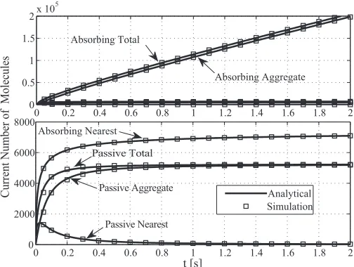
In Figs. 2, 3, and 4, we setNtx= 104, andkd= 0to focus
on normal diffusion without molecule degradation in a large-scale system. The analytical curves of the expected number of molecules absorbed at the absorbing receiver due to all transmitters, the nearest transmitter, and the other transmitters are plotted using (26), (21), and (22), and are abbreviated as “Absorbing All”, “Absorbing Nearest”, and “Absorbing Aggregate”, respectively. The analytical curves of the expected number of molecules observed inside the passive receiver due to all transmitters, the nearest transmitter, the other transmitters are plotted using (25), (21), and (22), and are abbreviated as “Passive All”, “Passive Nearest”, and “Passive Aggregate”, respectively. The analytical curves and the simulations are occasionally abbreviated as “Anal.” and “Sim.”, respectively.
A. Validation of Simulation Approaches
[image:10.612.54.302.504.555.2]by Brownian motion, and checking whether each molecule dif-fused into the passive receiver or was absorbed by the absorbing receiver. AcCoRD simulations are defined by configuration files; here, each configuration file listed the transmitter locations as specified by the current permutation of the HPPP, and each transmitter permutation was simulated at least 10 times.
The simulation approaches are compared in Fig. 2, where we setD= 80×10−12m2
s and assume that the transmitters are
placed up toRa = 50µm from the center of the receiver at a
density ofλa= 10−4transmitters perµm3(i.e., 52 transmitters
on average, including the exclusion of the receiver volume). The receiver takes samples everyTss = 0.01s and calculates
the net changein the number of observed molecules between samples. The default simulation time step is also0.01s. Unless otherwise noted, all simulation results were averaged over104
transmitter location permutations, as shown in Table II. In Fig. 2, we verify the analytical expressions for the expected net number of molecules observed during[t, t+Tss]at
both receivers in (21), and (22) by comparing with the particle-based simulations and the Monte Carlo simulations. In the right subplot of Fig. 2, we compare passive and absorbing receivers and observe the expected net number of observed molecules during [t, t+Tss] due to the nearest transmitter and due to
the other transmitters. In the left subplot of Fig. 2, we lower the simulation time step to 10−4s for the first few samples
of the two absorbing receiver cases, in order to demonstrate the corresponding improvement in accuracy. All curves in both subplots are scaled by the maximum value of the corresponding analytical curve in the right subplot; the scaling values and other simulation parameters are summarized in Table II.
1) Particle-Based Simulation Validation: Overall, there is good agreement between the analytical curves and the particle-based simulations in the right subplot of Fig. 2. The analytical results for the net number of molecules observed inside the passive receiver during[t, t+Tss]due to the nearest transmitter
are highly accurate, and even captures the net loss of molecules observed aftert= 0.1s. The particle-based simulation of the “Passive Aggregate” case also becomes noisier with increasing t as the normalized net number of molecules goes below 0.3, which is due to the very low number of molecules observed (the scaling factor in this case is only 9.525; see Table II) and can be improved by averaging over more realizations. Both simulation approaches slightly underestimate the analytical curve in the “Passive Aggregate” case for t < 0.1 s, due to the constraint on the placement of transmitters to within a radius ofRa = 50
µm (which we relax in later figures once we do not include particle-based simulations).
There is less agreement between the particle-based simula-tions and the analytical expressions for the absorbing receiver, and this is primarily due to the large simulation time step (even though we used a smaller time step for the aggregate transmitter case in the right subplot; see Table II). To demonstrate the impact of the time step, the left subplot shows much better agreement for the absorbing receiver model by lowering the time step to10−4s. This improvement is especially true in the
case of the nearest transmitter, as there is significant
devia-0 0.2 0.4 0.6 0.8 1 1.2 1.4 1.6 1.8 2
0 0.5 1 1.5
2x 10 5
0 0.2 0.4 0.6 0.8 1 1.2 1.4 1.6 1.8 2
0 2000 4000 6000 8000
t [s]
Analytical Simulation Passive Total
Passive Nearest Passive Aggregate
Absorbing Aggregate
Absorbing Nearest Absorbing Total
Curre
nt
N
um
be
r of M
ol
ec
ul
es
[image:11.612.313.565.52.242.2]
Fig. 3. Expected number of molecules observed at the receiver as a function of time.
tion between the particle-based simulation and the analytical expression for very early times in the right subplot.
2) Monte Carlo Simulation Validation: There is a good match between the analytical curves and the Monte Carlo sim-ulations for the net number of molecules observed at both types of receivers during [t, t+Tss] due to the nearest transmitter,
which can be attributed to the large number of molecules (as shown in Table II) and the small value of the shortest distance between the transmitter and the receiver compared withRa = 50µm. There is slight deviation in the Monte Carlo
simulations for the expected number of molecules observed at both types of receivers due to the other transmitters, and this is primarily due to the restricted placement of transmitters to the maximum distance Ra = 50µm. In Figs. 3 and 4, better
agreement between the analytical curves and Monte Carlo simulation is achieved by increasing the maximum placement distanceRa.
Due to the extensive computational demands to simulate such large molecular communication environments, we assume that the particle-based simulations have sufficiently verified the analytical models. The remaining simulation results in the rest of the figures are only generated via Monte Carlo simulation.
B. Channel Impulse Response Evaluation
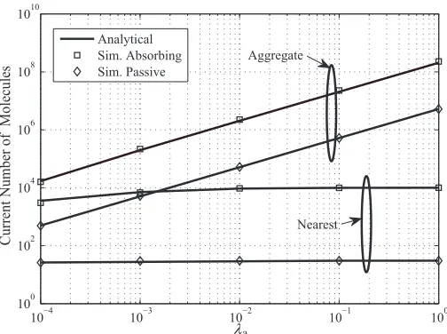
From Fig. 2 and the scaling values in Table II, we see that the expected net number of molecules observed at the absorbing receiver is much larger than that inside the passive receiver, since every molecule arriving at the absorbing receiver is permanently absorbed. We also notice that the expected net number of observed molecules due to the nearest transmitter is much larger than that due to the other transmitters, which may be due to a relatively low transmitter density.
10−4 10−3 10−2 10−1 100 100
102 104 106 108 1010
Analytical Sim. Absorbing Sim. Passive
Aggregate
Nearest
a
λ
Curre
nt
N
um
be
r of M
ol
ec
ul
es
[image:12.612.47.299.51.239.2]
Fig. 4. Expected number of molecules observed at the receiver at timet= 2 s as a function of the density of transmitters.
0.2 0.4 0.6 0.8 1 1.2 1.4 1.6 1.8 2
0.5 1 1.5 2 2.5 3
0.2 0.4 0.6 0.8 1 1.2 1.4 1.6 1.8 2
0.04 0.06 0.08 0.1 0.12
t[s]
Anal. Anal. Asymptotic Simulation Passive Total
Passive Total
Absorbing Asymptotic Absorbing Net
Absorbing Asymptotic Absorbing Net
a
λ
a
λ
Curre
nt
N
um
be
r of M
ol
ec
ul
es
N
et
N
um
be
r of M
ol
ec
ul
es
10−6 = 5x
10−5 = 1x
Fig. 5. Expected net number of molecules observed at the receiver as a function of time.
sampling interval. In Figs. 3 and 4, we set the parameters: D = 120×10−12m2
s , Ra = 100µm, and Tss= 0.1s. We set
the density of transmitters as λa = 10−3/µm3. As shown in
the lower subplot of Fig. 3, even though the point transmitters have random locations, the channel responses of the receivers due to the nearest transmitter in this large-scale molecular communication system are consistent with those observed at the absorbing receiver in [9, Fig. 4] and the passive receiver in [4, Fig. 2] and [22, Fig. 1] for a point-to-point molecular communication system.
In Fig. 3, we notice that the expected number of molecules currently observed at timetdue to all transmitters is dominated by the other transmitters, rather than the nearest transmitter, which is due to the increased number of molecules received from the other transmitters with the higher density of trans-mitters compared to that in Fig. 2. Furthermore, as we might
1 2 3 4 5 6 7 8 9 10
0 0.05 0.1 0.15 0.2 0.25 0.3 0.35 0.4 0.45 0.5
S
ingl
e Bi
t E
rror P
roba
bi
li
ty
Anal.
Anal.
Simulation Passive
Absorbing
= 1x 10a
λ
= 5a
λ
N th
x 10-5 -5
Fig. 6. Single bit error probability as a function of threshold.
[image:12.612.313.565.51.237.2]expect, the expected number of molecules currently observed inside the passive receiver at time t stabilizes aftert = 0.8s, whereas that at the absorbing receiver eventually increases lin-early with increasing time. This reveals the potential differences in appropriate demodulation design for these two types of receiver. More specifically, unlike the demodulation for passive receiver, demodulation using the number of molecules currently absorbed by the absorbing receiver is not a suitable design, since it cannot have a single optimal threshold.
Fig. 4 plots the expected number of molecules observed at the absorbing receiver and the passive receiver att= 2s versus the density of transmitters λa. With the increase of λa, the
number of observed molecules due to the other transmitters increases, whereas the number of observed molecules due to the nearest transmitter remains almost unchanged. More importantly, the dominant effect of the other transmitters on the number of observed molecules becomes more obvious as λa increases.
C. Demodulation Criteria and Single Bit Error Performance
From Figs. 3 and 4, the current number of absorbed molecules increases with increasing time and transmitter den-sity, thus demodulation based on the current number of molecules absorbed by the absorbing receiver will require an increasing demodulation threshold for largertandλa. Hence,
in our model, the demodulation of the absorbing receiver is based on the net number of absorbed molecules, whereas the demodulation of the passive receiver is based on the current
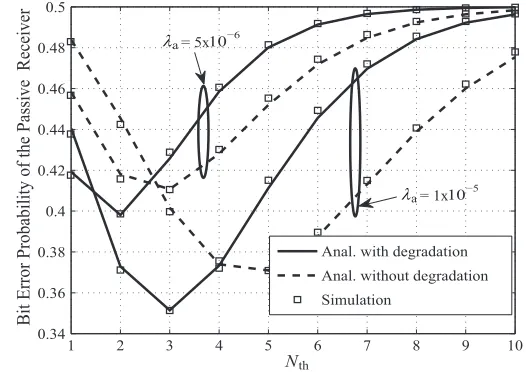
number of molecules observed at the receiver. In Figs. 5 and 6, we set Ntx = 20, kd = 0, Tb = 0.2 s, Ra = 100µm,
D = 80×10−11m2
s , and with only a single bit-1 transmitted
att= 0, i.e., the transmit bit sequence is [1 0 0 0. . .]. Fig. 5 plots the net number of molecules absorbed by the absorbing receiver during one bit interval Tb in the upper
[image:12.612.46.299.289.475.2]1 2 3 4 5 6 7 8 9 10 0.32
0.34 0.36 0.38 0.4 0.42 0.44 0.46 0.48 0.5
Anal. with degradation
Anal. without degradation
Simulation
Bi
t E
rror P
roba
bi
li
ty of t
he
A
bs
orbi
ng Re
ce
ive
r
10−5 = 1x
a
λ 10−6 = 5x
a
λ
[image:13.612.305.568.53.239.2]N th
Fig. 7. Bit error probability of the absorbing receiver as a function of threshold.
each with different transmitter densities. We also plot the asymptotic net number of absorbed molecules using (28) with a dashed line. We see that the net number of molecules absorbed by the absorbing receiver during each bit interval decreases as time increases, and converges to the asymptotic value. The number of observed molecules inside the passive receiver at the end of every bit interval remains comparable as time increases, which suggests that taking multiple samples of the number of observed molecules at different times in one bit interval may not greatly improve the detection reliability. For both receivers, the ISI is not small compared with the observation in the first bit interval, which demonstrates the high ISI in the large-scale molecular communication system.
In Fig. 6, we start using the second Monte Carlo approach for simulations in order to generate distributions of observations, and we plot the single bit error probability of both receivers using (36), in order to focus on the impact of multiple trans-mitters with no ISI impairment. We notice that the single bit error probability at both receivers improves with increasingλa,
which is due to the increased number of molecules absorbed by the absorbing receiver duringt∈[0, Tb], and the increased
number of observed molecules inside the passive receiver at t = Tb as seen in Fig. 5. Another interesting observation is
that the single bit error probability of the passive receiver is much worse than that of the absorbing receiver, which is due to the lower number of observed molecules at the passive receiver than that at the absorbing receiver. Clearly, the two receivers need different demodulation thresholds.
D. Multiple Bits Error Performance
Figs. 7 and 8 plot the bit error probabilities of the absorbing receiver and that of the passive receiver in the proposed large-scale molecular communication system, respectively, both with
(kd= 0.8s−1)or without(kd= 0s−1)molecule degradation.
Fig. 9 compares the bit error probabilities of the absorbing receiver and the passive receiver in the proposed large-scale
1 2 3 4 5 6 7 8 9 10
0.34 0.36 0.38 0.4 0.42 0.44 0.46 0.48 0.5
Bi
t E
rror P
roba
bi
li
ty of t
he
P
as
si
ve
Re
ce
ive
r
Anal. with degradation
Anal. without degradation
Simulation
N th
10−6 = 5x
a
λ
10−5 = 1x
a
[image:13.612.57.417.54.238.2]λ
Fig. 8. Bit error probability of the passive receiver as a function of threshold.
molecular communication system under molecule degradation
(kd= 0.8s−1)using DFD, with that using the simple detector.
In Figs. 7, 8, and 9, we set the parameters: Tb = 0.2 s,
Ra = 100µm, andD = 80×10−11m
2
s with a 5 bit sequence
transmitted by all transmitters, where the first four bits are set as [1 0 1 0] . We setNtx= 20in Fig. 7,Ntx= 300in Fig. 8,
andNtx= 104 in Fig. 9.
In Figs. 7 and 8, we see a good match between the analytical results in (36) and the simulations, which demonstrates the correctness of our derivations. We observe that the minimum bit error probability improves with increasing the density of the transmitters. We also see that the minimum bit error probability can be improved by introducing molecule degradation. This can be explained by the fact that many molecules, especially those released far from the receiver, degrade before they reach the receiver, and this reduces the ISI effect. However, the bit error probability with molecule degradation is not always better than without degradation for a given decision threshold, which can be attributed to the fact that the degradation not only reduces the ISI, but also lowers the strength of the intended signal.
In both figures, we notice that the minimum bit error probability is still not low enough for reliable transmission, even though it can be potentially improved by increasingNtx.
This is because with multiple transmitted bits, the ISI will accumulate and keep growing with every transmit bit-1. These observations reveal that the demodulation threshold at each bit should increase with the number of transmit bits, instead of being fixed.
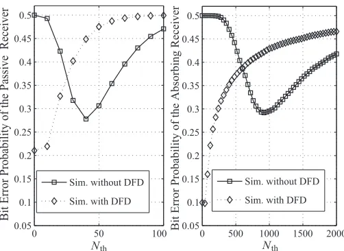
We now consider the DFD at both receivers to show its potential benefits in improving the bit error probability. Fig. 9 compares the bit error probability of both receivers having molecule degradation during diffusion and DFD during detec-tion with that without DFD during detecdetec-tion using Monte Carlo simulation, where the passive receiver is capable of subtracting the current observation in one previous bit interval N[j−1]
0 500 1000 1500 2000 0.05
0.1 0.15 0.2 0.25 0.3 0.35 0.4 0.45 0.5
0 50 100
0.05 0.1 0.15 0.2 0.25 0.3 0.35 0.4 0.45 0.5
Sim. without DFD
Sim. with DFD
Sim. without DFD
Sim. with DFD
Bi
t E
rror P
roba
bi
li
ty of t
he
A
bs
orbi
ng Re
ce
ive
r
Bi
t E
rror P
roba
bi
li
ty of t
he
P
as
si
ve
Re
ce
ive
r
[image:14.612.47.298.51.234.2]N th N th
Fig. 9. Bit error probability of receivers as a function of threshold.
receiver is capable of subtracting the net observation in one previous bit interval N[j−1] from that in the current bit intervalN[j] for the demodulation of thejth bit. With DFD, the jth bit is decoded based on if N[j]−N[j−1] > Nth
or not. By doing so, the accumulated ISI due to the previous bits is mitigated artificially during the demodulation process. We set λa = 5×10⁻⁶/µm3. With the help of DFD, we see
that the minimum bit error probability of both receivers can be improved for the proposed system.
VII. CONCLUSIONS ANDFUTUREWORK
In this paper, we provided a general model for the collective signal modelling in a large-scale molecular communication system with or without degradation using stochastic geometry. The collective signal strength at a fully absorbing receiver and a passive receiver is modelled and explicitly characterized. We derived tractable expressions for the expected number of observed molecules at the fully absorbing receiver and the passive receiver, which were shown to increase with transmitter density. We also derived analytical expressions for the bit error probabilities at both receivers with a simple detector taking one sample per bit, and the minimum bit error probabilities were shown to improve with the help of degradation. The analytical model presented in this paper can also be applied for the performance evaluation of other types of receiver (e.g., partially absorbing, reversible adsorption receiver, ligand-binding receiver) in a large-scale molecular communication system by substituting its corresponding channel response.
APPENDIXA PROOF OFPROPOSITION1
According to [33], the probability of finding k nodes in a bounded Borel A ⊂ Rm in a homogeneous m-dimensional Poisson point process of intensityλis given by
Pr (M =k) =e−λaµ(A)(λaµ(A))k
k! , (A.1)
where M is the Poisson random variable, and µ(A) is the standard Lebesgue measure ofA.
Thus, the probability of finding zero nodes in a bounded BorelA⊂R3 in a homogeneous3D Poisson point process of intensityλa is obtained as
Pr (M = 0) =e−λaµ(A), (A.2)
where µ(A) = 43πx3−4
3πrr3, and x is the radius of the
bounded ball.
Usingfkx∗k(x) =−dPr(dxN=0), we prove (19).
APPENDIXB PROOF OFTHEOREM1
Based on (8) and (18), we can write the expected net number of molecules observed at the receiver as
E{Nall(Ωrr, t, t+Tss)}=E
n X
x∈Φa
NtxΦ (r)
o
, (B.1)
where
Φ (r) =FFA( Ωrr, t, t+Tss|r), (B.2)
for the absorbing receiver, and
Φ (r) =FPS( Ωrr, t+Tss|r)−FPS( Ωrr, t|r), (B.3)
for the passive receiver.
According to the Campbell’s theorem in 3D space, the mean of the random sum of a point processΦa onR3 andNtxΦ (r)
is given as [24, Eq. (1.18)]
E{Nall(Ωrr, t, t+Tb)}=
Z
R3
[NtxΦ (r)]λadx
=λa
Z ∞
rr
[NtxΦ (r)] 3
4π
3 r
2dr. (B.4)
Thus, we derive
E{Nall(Ωrr, t, t+Tss)}= 4πλaNtxFA
Z ∞
rr
Φ (r)r2dr. (B.5)
APPENDIXC PROOF OFLEMMA1
Withkd= 0, we rewrite (B.5) usingz=r−rr as
ENallFA(Ωrr, t, t+Tss) = √
4πλaNtxrr √
D
Z t+Tss
t
Z ∞
0
z(z+rr) exp −
z2
4Dx
dz√1
x3dx
=
√
4πλaNtxrr √
D
"Z t+Tss
t
Z ∞
0
z2exp − z
2
4Dx
dz√1
x3dx
+rr
Z t+Tss
t
Z ∞
0
zexp − z
2
4Dx
dz√1
x3dx
#