Planning Models
Emma Ross
Submitted for the degree of Doctor of
Philosophy at Lancaster University.
Cross-training has emerged as an effective method for increasing workforce flexibility
in the face of uncertain demand. Despite recently receiving substantial attention in
workforce planning literature, a number of challenges towards making the best use of
cross-training remain. Most notably, approaches to automating the allocation of workers
to their skills are typically not scalable to industrial sized problems. Secondly, insights
into the nature of valuable cross-training actions are restricted to a small set of
pre-defined structures.
This thesis develops a multi-period cross-trained workforce planning model with
temporal demand flexibility. Temporal demand flexibility enables the flow of incomplete work (orcarryover) across the planning horizon to be modelled, as well as an the option to utilise spare capacity by completing some work early. Set in a proposed Aggregate Planning stage, the model permits the planning of large and complex workforces over a horizon of many months and provides a bridge between the traditional Tactical and
Operational stages of workforce planning. The performance of the different levels of
planning flexibility the model offers is evaluated in an industry motivated case study.
An extensive numerical study, under various supply and demand characteristics, leads
to an evaluation of the value of cross-training as a supply strategy in this domain.
The problem of effectively staffing a pre-fixed training structure (such as the modified
chain or block) is an aspect of cross-training which has been extensively studied in the
literature. In this thesis, we attempt to address the more frequently faced problem
of ‘how should we train our existing workforce to improve demand coverage?’. We
propose a two-stage stochastic programming model which extends existing literature
by allowing the structure of cross-training to vary freely. The benefit of the resulting
targeted training solutions are shown in application using a case study provided by BT. A wider numerical study highlights ‘rules-of-thumb’ for effective training solutions under
support, supplied in few words but many actions.
Firstly, I’d like to thank my supervisor Chris Kirkbride for his guidance and the faith he
has shown in me throughout this process. Further thanks go out to my supervisors at
BT: Sid Shakya and Gilbert Owusu. Their enthusiasm and ambition spurred me on in
my research, contributing to a valuable experience of innovation in industry. Fortunate
enough to win funding to collaborate with external academic institutions, special thanks
go out to Stein Wallace for hosting me at the Norwegian School of Economics. Meetings
with Stein were lively and fun but also extremely useful and I am grateful to have had
the chance to learn from him.
I gratefully acknowledge the financial support of the EPSRC through a studentship
within the STOR-i Centre for Doctoral Training. My PhD experience surpassed
expec-tations due to the support and encouragement of peers and staff members at Lancaster
University. It was a pleasure to study with such a diverse group of friendly people.
Last but certainly not least, I would like to thank those closest to me outside of the
STOR-i family. Thank you to my boyfriend James whose encouragement and support
has been unwavering throughout my time at Lancaster. I hope that I can find a way to
support him, as he has me, in his own future endeavours. I would also like to thank my
family who, very much to my appreciation, have rarely dared to ask ‘Have you finished
the PhD yet?’. Your advice in the challenging final stages of writing was spot on, I
couldn’t have done it without you.
I declare that the work in this thesis has been done by myself and has not been submitted
elsewhere for the award of any other degree.
Emma Ross
Abstract I
Dedication III
Acknowledgements IV
Declaration V
Contents VI
List of Figures VII
List of Tables VII
1 Introduction to Workforce Planning 1
1.1 Workforce Planning . . . 1
1.1.1 Industry Motivation . . . 3
1.1.2 Aggregate Planning . . . 6
1.2 Thesis Outline . . . 6
2 Core Methodology 8 2.1 Introduction . . . 8
2.2 Univariate Time series . . . 8
2.2.1 Time Series Decomposition . . . 9
2.2.2 Modelling Stationary Residual Variation . . . 10
2.2.3 Change-point Detection . . . 14
2.3 Multivariate Dependence Modelling . . . 17
2.3.1 The Copula Function . . . 17
2.3.2 Examples of Useful Copulas . . . 18
2.3.3 Extremal Dependence . . . 26
2.4 Stochastic Linear Programming . . . 30
2.4.1 Decision Problems as Linear Programs . . . 31
2.4.2 Stochastic Linear Programming . . . 33
2.4.3 Scenario Generation . . . 36
3 Demand Modelling 39 3.1 The Data . . . 40
3.2 Univariate Modelling . . . 41
3.3 Multivariate Modelling . . . 48
3.3.1 Data Exploration . . . 49
3.3.2 Fitting Bivariate Copulas . . . 52
3.3.3 Comparison of Model Fit . . . 55
3.4 Multivariate Demand Simulation . . . 60
3.4.1 Multivariate Scenario Generation . . . 63
3.A Chapter 3 Appendix . . . 64
3.A.1 Two-dimensional Kernel Density Estimation . . . 64
3.A.2 Simulation from a Multivariate Copula . . . 65
4 Workforce Planning with Carryover 68
4.1 Introduction . . . 68
4.2 Literature Review . . . 72
4.3 An Aggregate Cross-trained Workforce Planning Model with Temporal Demand Flexibility . . . 77
4.3.1 The Aggregate Planning Model . . . 82
4.3.2 Model Variants . . . 87
4.4 Case Study . . . 89
4.4.1 Study Design . . . 89
4.4.2 Study Results . . . 94
4.5 Extended Numerical Study . . . 101
4.5.1 Environmental Factors and Study Design . . . 101
4.5.2 Performance Analysis: Environmental Effects . . . 106
4.5.3 The Cost of Completing Work Early . . . 113
4.6 Conclusions and Future Work . . . 117
5 Cross-training Policies & Stochastic Demand 120 5.1 Introduction . . . 120
5.2 Modelling . . . 125
5.2.1 Allocation and the Carryover of Incomplete Work . . . 126
5.2.2 Model Stochastics . . . 127
5.2.3 Two-stage Training Model . . . 134
5.3 Case Study . . . 141
5.3.1 Demand Modelling . . . 141
5.3.2 Setting Supply . . . 144
5.3.3 Setting Training Cost ki . . . 145
5.3.5 Case Study Results . . . 150
5.4 Extended Numerical Study . . . 157
5.4.1 Environmental and Experimental Factors . . . 157
5.4.2 Numerical Study Results . . . 160
5.4.3 Discussion and Managerial Insights . . . 167
5.5 Conclusion . . . 168
1.1.1 Four-stage workforce planning hierarchy for large scale service industries 2
2.3.1Surface and contour plots of the cumulative distribution function for the
bi-variate independence copula . . . 20
2.3.2Surface and contour plots of the cumulative distribution function for the
bi-variate perfect dependence copula . . . 20
2.3.3Surface and contour plots of the cumulative distribution function for the
Gaus-sian dependence copula. . . 22
2.3.4Surface and contour plots of the cumulative distribution function for the
logis-tic extreme value copula . . . 26
2.3.5Extremal dependence measure χl(u) for the bivariate logistic extreme value
copula: solid lines (bottom to top) correspond to α = 0.9,0.8, . . . ,0.1 and
dashed lines give the bounds of χl(u) . . . 29
2.3.6Extremal dependence measure χl(u) for the bivariate Gaussian copula: solid
curves (bottom to top) correspond to correlation coefficientρ=−0.9,−0.8, . . . ,0.9 and dashed curves give the bounds ofχl(u). . . 29
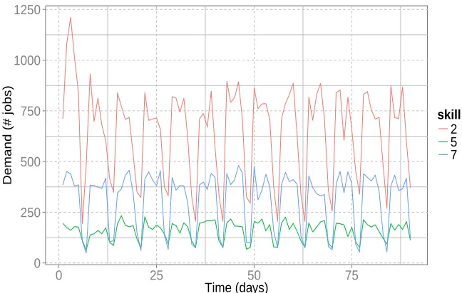
3.1.1Sample of Case-study Historic Demand . . . 40
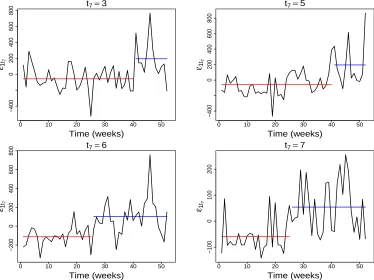
3.2.1Step-change in empirical residual variation in demand for skill 1, ε1t7, under
time series model 3.2.1 . . . 43
3.2.2Case study data example for a single demand skill . . . 47
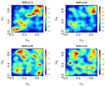
3.3.1 Pairwise 2-D kernel density plots . . . 50
3.3.2Comparison of extremal dependence measure χ(u) for the Gaussian copula
model (blue) and logistic extreme value copula (magenta) along with empirical
χ(u) (black) with 95% confidence limits . . . 57
3.3.3Comparison of extremal dependence measure χl(u) for the Gaussian copula
model (blue) and logistic extreme value copula (magenta) along with empirical
χl(u) (black) with 95% confidence limits . . . 58
4.1.1 Four-stage workforce planning hierarchy for large scale service industries 69
4.4.1 Case study data example: subplot (a) illustrates a time series of demand
for skill 6 while subplot (b) illustrates an sGE distribution fitted to
ran-dom variation around the cyclic component of demand for the same skill 91
4.4.2 Case Study: boxplots of percentage reduction in terminal cumulative
demand carryover for strategies π ∈ Π\Ba, relative to strategy Ba, by
early completion limit . . . 95
4.4.3 Mean percentage reduction in terminal cumulative demand carryover for
strategies Ca and Ea, relative to strategy Ba, as a function of planning
horizon length. The solid line represents the value of using strategy Ca.
The dashed line represents the value of using strategy Ea with an
early-completion limit, lj, of 1 day . . . 96
4.4.4 The evolution of cumulative demand carryover throughout a planning
horizon for a single problem instance and demand realisation . . . 98
4.5.1 Numerical Study: boxplots of percentage reduction in terminal
cumula-tive demand carryover for strategies π ∈ Π\Ba, relative to strategy Ba,
by early completion limit . . . 108
4.5.2 Mean percentage of demand completed early by early completion cost . . 116
5.3.1 Case study data example: subplot (a) illustrates a time series of demand
for skill 6 while subplot (b) illustrates an sGE distribution fitted to
ran-dom variation around the cyclic component of demand for the same skill 143
5.3.2 Proportion of the total workforce trained for a range of training costs ki,
with carryover costcj = 1 for all j ∈J. The solid line corresponds to the
case study. The dotted line corresponds to an equivalent problem with
inflated variation in demand and negative cross-correlation. The dashed
line corresponds to a lower-variation and positive correlation case. . . 146
5.3.3 Box-plots of the benefit of utilising cross-training over 100 simulations. TS 1 corresponds to a training solution resulting from one repetition of
the training model. Plot (a) demonstrates the benefit of cross-training
when the carryover of incomplete work through time is not included in the
allocation. Plot (b) is equivalent but with carryover included in allocation.152
5.3.4 Quantity of FTE workers trained into a new worker type defined by skill
vector “j, k” where j is their primary skill and k their secondary skill.
Sub-figure (a) picks a random sample of 5 training solutions to illustrate,
distinguishable by the shade of bars plotted. Sub-figure (b) summarises
100 repetitions of the training model with box-plots for each worker type.
The shade of box-plots relates to the cross-correlation between the skills
combined in the worker type. . . 154
5.3.5 Plot illustrating the mean and variance properties of demand for skills
combined in training. Each intersection of 2 dashed lines represents a
worker class we might train into (defined by skills paired-up in training).
Larger points plotted reflect a larger number of workers trained into that
5.4.1 Quantity of FTE workers trained into a new worker type defined by skill
vector “j, k” where j is their primary skill and k their secondary skill.
Box-plots summarise 100 replications of the training model applied to a
problem instance with zero cross-correlation; low standard deviation; low
skewness and kurtosis; and training cost ki = 1.3 . . . 164
5.4.2 Bar plots of the change in quantities of worker types trained caused by
introducing non-zero correlation. Comparison is made against a baseline
solution for 0 correlation; high variation and low skewness and kurtosis
common to all skills. . . 165
5.4.3 Bar plot of the change in quantities of worker types trained caused by
introducing demand variation which differs across skills. Comparison is
made against a baseline solution for 0 correlation; high variation and low
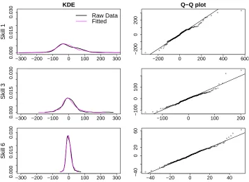
3.2.1 Skewed Generalised Error distribution parameters fitted for random
vari-ation in weekday demand, Ed
1,E3d and E6d, for skills 1,3 and 6. . . 46 3.3.1 Spearman’s correlation coefficientrs for all pairs of skills. . . 51
3.3.2 95% bootstrap confidence intervals for Spearman’s correlation coefficient
rs (calculated with 100 bootstrap re-samples). . . 51
3.3.3 Maximum likelihood estimates for bivariate Gaussian copula parameters
ˆ
ρij where (i, j)∈J×J . . . 55
3.3.4Maximum likelihood estimates for bivariate logistic extreme value copula
pa-rameters ˆαij where (i, j)∈J×J . . . 55
3.3.5 Percentage improvement, D, in maximum likelihood resulting from a
Gaussian copula over an extreme value copula model for bivariate data
defined by pairs of skills. Positive values give the percentage improvement
in Gaussian maximum likelihood value,LG( ˆρ), above the logistic extreme
value equivalent, LE( ˆα). Negative values have an analogous meaning in
the other direction (improved likelihood under the logistic extreme value
copula over the Gaussian copula) . . . 59
4.3.1 Model notation . . . 81
4.4.1 Worker class efficiency matrix defining a modified chain cross-training
structure for 4 skills with a training depth of 2. Rows describe the abilities
(efficiencies) of worker class i in skills j ∈ {1, . . . ,4}.. . . 93
4.4.2 Case Study: mean (standard error) percentage reduction in terminal
cu-mulative demand carryover for strategies π ∈Π\Ba, relative to strategy
Ba, by early completion limit . . . 94
4.5.1 Experimental and environmental factors and levels . . . 102
4.5.2 Example worker class efficiency weight matrices for different cross-training
structures . . . 105
4.5.3 Numerical Study: mean (standard error) percentage reduction in
termi-nal cumulative demand carryover for strategies π ∈ Π\Ba, relative to
strategy Ba, by early completion limit . . . 107
4.5.4 Mean (standard error) percentage reduction in terminal cumulative
de-mand carryover for strategies π ∈ Π\Ba, relative to strategy Ba, by
coefficient of variation . . . 109
4.5.5 Mean (standard error) percentage reduction in terminal cumulative
de-mand carryover for strategies π ∈ Π\Ba, relative to strategy Ba, by
cross-correlation . . . 110
4.5.6 Mean (standard error) percentage reduction in terminal cumulative
de-mand carryover for strategies π ∈ Π\Ba, relative to strategy Ba, by
AR(1) dependence . . . 111
4.5.7 Mean (standard error) percentage reduction in terminal cumulative
de-mand carryover forCT-type strategies, relative to strategyBa, by breadth
4.5.8 Mean (standard error) percentage reduction in terminal cumulative
de-mand carryover for CT-type strategies, relative to strategyBa, by
train-ing structure and configuration . . . 112
4.5.9 Mean (standard error) percentage reduction in terminal cumulative
de-mand carryover for Ea-type strategies, relative to strategy Ba, by early
completion cost . . . 114
5.2.1 Model notation . . . 135
5.3.1 Illustration of the modified chain cross-training structure with training
depth of 2 and number of skills |J|= 4. The matrix contains efficiency
weightswij with rows representing worker classes and columns
represent-ing skills. . . 149
5.4.1 Experimental and environmental factors and levels . . . 159
5.4.2 Mean benefit of targeted and modified chain training solutions, measured
in % of incomplete work removed due to utilising cross-training. The
standard error of estimates is parenthesised. Results correspond to ki =
1.3, low kurtosis κj, and low positive skewness λj. . . 161
5.4.3 Mean proportion of the workforce trained as a result of targeted training
measured in %. The standard error of estimates is parenthesised. Results
Introduction to Workforce Planning
1.1
Workforce Planning
The effective planning and deployment of an organisation’s workforce plays a vital role
within service industries. Delivery of services relies primarily on an expensive human
workforce which often accounts for a large proportion of overall running costs.
Success-ful organisations can establish a competitive edge by careSuccess-fully planning human resources
so that delivery is timely to demand (Owusu and O’Brien, 2013). This planning must
also account for the need to preserve the existing workforce by providing fair working
conditions and ensuring breaks and personal preferences for work are factored into
de-cisions. Pokutta and Stauffer (2009) argue that in increasingly competitive markets,
this challenge has become paramount for the maximisation of profit and, increasingly,
to ensure the survival of organisations.
Human resource planning problems are often misconceived to concern only
short-term scheduling decisions such as ‘what is the optimal tour of a particular engineer
given a set of tasks for the day?’. To provide a quality service at low operational cost, a
workforce schedule with this degree of detail is sought as an end product to the planning
process. The final scheduling solution is only as effective as the planning decision which
Strategic Planning
Tactical Planning
Aggregate Planning
Operational Planning
What: Location and number of service cen-tres; staff ratios
When: 1-2 years in advance
What: Hiring; training; volume of demand to be met
When: 12-18 months in advance
What: Aggregate allocation of workers’ skills to demand for those skills
When: 1 to 90 days in advance
What: Scheduling and assignment of individ-ual workers to tasks
When: Beginning of week or shift
Figure 1.1.1: Four-stage workforce planning hierarchy for large scale service industries
came before it, however. If the supply-demand inputs to scheduling (a fixed quantity
of workers and jobs for a given day) are imbalanced, there is little that any scheduling
decision can do to rectify it.
Indeed, coordinating workforces encompassing more than a few tens of workers
quickly becomes a daunting task. A typical approach to simplifying resource
plan-ning problems is to break the problem down into a sequence of interconnected stages of
decision making. Figure 1.1.1 presents a planning hierarchy containing three common
planning stages: Strategic; Tactical and Operational Planning.
Strategic Planning involves the highest level decisions about the scope of the
activ-ities of the organisation, typically made years ahead of operations. Tactical Planning
describes the actions required to achieve the plans set out in Strategic Planning, in
this case, the annual or bi-annual setting of required staffing levels and training. The
Operational Planning stage is then concerned with the day-to-day scheduling of the
resulting workforce and takes as input the configuration of supply resulting from the
previous Tactical Planning stage. An important consideration when planning using such
In the following section we provide background on the industry problem which
mo-tives the thesis. The above planning hierarchy proves useful in framing the challenges
faced by the associated organisation. This motivates the identification of an additional
aggregate planning level, the definition and reasoning for which is provided later in the chapter.
1.1.1
Industry Motivation
Large service organisations, such as utility and telecommunications companies, typically
rely on large workforces. They are responsible for the maintenance and repair of their
existing infrastructure as well as for the role-out of new developments. For example, BT,
a world leading telecommunications service company and one of the leading
telecom-munications providers in the UK, have an engineering workforce of around 22,000. To
maintain network reliability and customer satisfaction, the workforce must be planned
carefully so that sufficient worker numbers are available to meet uncertain demand at
any time. Establishing the quantity of resources needed for each planning period is
an every-day task but one which is extremely complex with great cost implications to
the company if poorly resolved. In particular, over-supply leads to unnecessary human
resource expense while service level agreements can be breached and fines incurred with
under-supply.
Ensuring efficiency in this area is clearly well motivated but the task itself involves
numerous challenges, the most significant of which we now describe.
Demand Uncertainty
Typically, the process of assigning supply to demand can begin up to 3 months ahead of
operations, when knowledge of demand and hence the ability to make effective workforce
with last minute requests, cancellations and amendments to jobs with potentially very
little notice. Keeping up with ever-evolving demand is a challenge for every sector but
is one perhaps most prominent in the service industry. Production companies trading in
goods can buffer against demand uncertainty using inventories - keeping spare stock of
products in case of a peak in demand. For human resource intensive service industries
however, inventories are not an option and so the delivery of resources must be timely.
Early planning efforts, however approximate, allow imbalance between supply and
demand to be spotted and rectified in the run-up to operations when there is less
flexibility to make changes.
A common consequence of uncertain demand and limited resources is incomplete
work remaining at the end of a day. This demand does not go away, rather it
contin-ually gets added to demand on the following day until it can be completed. Workforce
planning models commonly disregard the propagation of incomplete work through time
in favour of assuming there are the resources to clear all work at the end of each working
day, e.g. via outsourcing or overtime. This luxury is rarely a reality, with late-running
work an unavoidable characteristic of demand in many service industries, including BT.
According to Owusu et al. (2006), effective resource planning under uncertainty is
critical to optimal service delivery in service organisations such as BT. It is of interest to
such companies to bring about robust resource capacity decisions which balance against
the risk of costs incurred from under- and over-supply. A key step towards ensuring
robustness of solutions is understanding how automated planning models perform under
a range of outcomes for demand. It is therefore vital that a mechanism exists for
simulating demand outcomes reflective of, but not identical to, historic demand.
Multi-skilled workforces
The challenges introduced by uncertainty in demand highlight the need for workforce
flexibility is cross-training so that some proportion of workers are able to work on two or
more types of task. Much research has gone into the benefits of multi-skilled workforces,
leading to recommendations for optimal training configurations in terms of breadth
(number of skills per employee) and depth (level of expertise in each skill) of training
within a fixed pattern. Though many companies have acted on these recommendations
by setting about building a multi-skilled workforce, they have not necessarily been able
to reap the benefits. The effective utilisation of this new-found flexibility relies upon
proactively allocating workers to their different skills.
Comparatively little work has been carried out on this multi-skilled workforce
allo-cation aspect of planning. Indeed, a common approach is to consider workers secondary
skills only once the scheduling stage has been reached, in an ad hoc manual adjustment
of individuals’ schedules to suit demand. Part of the contribution of this thesis is to
provide a method which automates the allocation of workers to their range of skills.
Problem Scale
Aligning a large workforce with demand for a wide range of skills leads to an extremely
large scale decision problem. Cross-training policies heighten the complexity of the
planning task, bringing about the combinatorial challenge of distributing a workforce
over a complex network of skills and varying ability levels.
Typically, consideration of how a cross-trained workforce’s flexibility can be exploited
is left until the final stages of assigning individuals to specific tasks within their skill-set.
The resulting assignment problem, as an extension of the NP-hard Generalised
Assign-ment Problem ( ¨Oncan, 2007; Heimerl and Kolisch, 2010), becomes computationally
1.1.2
Aggregate Planning
To improve and automate planning practices related to cross-trained workforces, we
propose that the allocation of workers to different skills is considered much earlier in
the planning horizon than scheduling in the Operational Planning level.
This motivates consideration of an Aggregate Planning stage, positioned at the in-terface between Tactical and Operational Planning of Figure 1.1.1, which contributes
to the effective deployment of large workforces with complex cross-training structures.
Taking as input the staffing and training decisions made in Tactical Planning, this
stage establishes an effective utilisation of groups of workers’ skills on an aggregate
level and quantifies the resulting accumulation of unmet demand (or carryover) across a planning horizon of a number of weeks. The result is a richer view of supply-demand
balance over the horizon and targets for the time workers spend on each skill. Schedules
can be then be built in the Operational Planning stage based on the output of Aggregate
Planning, resulting in a proactive, not reactive, exploitation of workers’ flexibility.
Though aggregate allocation models will lack detail on the level of the individual,
they have the benefit of being scalable to large and complex workforces and have more
scope to influence decision making and understanding in higher levels of the planning
hierarchy.
1.2
Thesis Outline
With the above motivation and problem background in mind, this thesis develops a
scalable approach to automating the allocation of cross-trained workers to demand for
their skills. This allocation model is then used to explore the impact of training actions
applied to an existing workforce - extending insights into the value of cross-training
These two key contributions are being prepared for publication and, as such, appear
as self-contained reports in Chapters 4 and 5. The reader should therefore expect some
repetition of introductory material. Details of the contents of each chapter are now
given.
A multi-period cross-trained workforce planning model is proposed for the Aggregate
Planning stage in Chapter 4. This model incorporates the flow of incomplete work across
the planning horizon and facilities measurement of the value of cross-training in this
carryover inclusive setting. The contents of this chapter have been submitted to the Journal of the Operational Research Society under title Ross, E., Kirkbride, C., Shakya, S., Owusu, G. Cross-trained workforce planning for service industries: The effects of temporal demand flexibility.
The allocation model is extended to the Tactical Planning level in the training model
proposed in Chapter 5. The two-stage stochastic programming model is used to explore
the interaction between the characteristics of uncertain demand and the nature of an
effective cross-training structure. The content of this chapter is presently being prepared
for submission toFlexible Services and Manufacturing under the title Ross, E., Wallace, S., Shakya, S., Owusu, G.Cross-training Policies for Service Industries: The Effects of Stochastic Demand.
Central to incorporating uncertainty in this training model and in testing the
ro-bustness of the allocation model is a procedure with which to simulate multivariate
time series realisations for demand. Chapter 3 documents the data analysis leading to
a simulation procedure. The core methodologies called upon in this work are outlined
Core Methodology
2.1
Introduction
In this chapter we introduce the key statistical and mathematical modelling methodology
drawn upon in this work.
2.2
Univariate Time series
A key measure of the success of a workforce planning strategy is its ability to cover
continually changing demand. Being able to model time series of historic demand
pro-vides an understanding of the market which can prove valuable in planning supply to
meet future demand. It is common practice to test how new approaches to workforce
planning would have performed against historic time series for demand. If we have a
time series model for that demand, we can further assess planning approaches under a
wider range of realisations characteristic, but not identical to, historic demand. This is
critical to the development of robust strategies which are proven against a future not
necessarily identical to the past.
In this section we describe a traditional approach to time series modelling and
tify stochastic processes which prove useful in modelling residual variation of a time
series. An approach to the detection of change-points in a time series is also described.
2.2.1
Time Series Decomposition
Hamilton (1994) identifies a time series to be a single outcome of some underlying
stochastic process. We define a discrete time stochastic process {Xt}t∈T to be a set of
random variables ordered in time and defined at a discrete set of time-pointst∈T.
Much of the probability theory of time series is applied to stationary time series, characterised by the joint distribution of (Xt1, . . . , Xtn) being the same as the joint
distribution of (Xt1+τ, . . . , Xtn+τ) for all τ and t1, . . . , tn ∈ T. Time series analysis
therefore often requires non-stationary series to be transformed to stationary series so
that their associated probability theory can be exploited.
The classical approach to time series analysis involves decomposing the variation in
a series into four key components: trendT; seasonal variation S; other cyclic variation
C; and residual variation ε. The goal is then to capture all systematic variation using
deterministic components T,S and C, to reach stationary residual variation ε.
We now describe these components in more detail. Many time series, such as daily
temperature recordings, exhibit cyclic variation S which is annual in period. Such
seasonal cyclic variation is often well-understood and can therefore be directly modelled
or removed from the data. As well as seasonal variation, shorter-term cyclic variationC
may be a feature of the time series, e.g. within-day temperature fluctuation. The trend
componentT is used to account for any long-term change in mean level. The meaning
oflong-term, and hence the differentiation between trend and a cyclic component with a long wave-length, depends on the application of interest. For the applications considered
in this work, we identify trend to be variation with period longer than one year. The
around the underlying trend and cyclic components.
To provide an example, we might summarise univariate stochastic process {Xt}t∈T
in terms of these components using the following additive model:
Xt =Tt+St+Ct+εt.
Provided we can find some model for stationary residual variationεt, new realisationsx
0
t
on the same intervalt ∈ {1, . . . ,|T|}can be generated by samplingεtfrom its model and
combining with deterministic components T,S and C. Note that the structure of the
decomposition need not be additive, indeed popular alternatives feature multiplicative
components.
The decomposition of a time series into such components is typically not unique,
unless some assumptions are made. This highlights the descriptive but also inferential
role that time series decompositions can play.
2.2.2
Modelling Stationary Residual Variation
We highlight two stationary stochastic processes which are useful in modelling residual
variationεt: white noise and autoregressive stochastic processes.
White Noise Process
A sequence of random variables {Zt}t∈T is a white noise process if its variables are
serially uncorrelated with zero mean and finite variance (Shumway and Stoffer, 2006).
In the case that its variables are also independent and identically distributed (i.i.d),
autocorrelation, so that
γ(k) = Cov(Zt, Zt+k)
= 0 for allk =±1,±2, . . .
When residual variation εt has the characteristics of white independent noise,
generat-ing a new time series realisation, {x01, . . . , x0|T|}, simply requires sampling ε0t from the distribution fitted to independent valuesεt.
Assuming all underlying trend and cyclic behaviour has been removed, εt can be
modelled using any suitable zero-centred distribution, also called anerror distribution. The normal distribution centred at zero is often suggested in the definition of time series
decomposition. Our motivating application calls for error distributions with thinner tails
or skewness not characteristic of the normal distribution, however. The skewed
Gener-alised Error (sGE) distribution offers the required flexibility to model these properties
and contains the normal distribution as a special case (Theodossiou, 2015). The sGE
distribution has the following probability density function:
f(x;µ, σ, k, λ) = C
σ exp
− |x−µ+δσ|
k
(1 + sign(x−µ+δσ)λ)kθkσk
where
C= k
2θΓ(1/k)
δ= 2λAG(λ)−1
θ= Γ(1/k)0.5Γ(3/k)−0.5G(λ)−1
G(λ) =√1 + 3λ2−4A2λ2
A= Γ(2/k)Γ(1/k)−0.5Γ(3/k)−0.5
δ= 2λAG(λ)−1.
We adopt the definition given by Bali and Theodossiou (2008) for its convenience in
writing computer code for both the distribution function and likelihood. Parametersµ
and σ are respectively the mean and standard deviation of random variable x; whilst
k is a positive valued kurtosis parameter and λ is a skewness parameter obeying the
constraint|λ|<1. In the above density, µ−δσ is the mode and δ= (µ− mode(x))/σ
is Pearson’s measure of skewness. The sGE distribution contains several well-known
distributions as special cases:
• λ = 0 gives the generalised error distribution or power exponential distribution of
Subbotin (1923);
• λ = 0, k = 2 gives the normal distribution;
• λ = 0, k = 1 gives the Laplace or double exponential distribution; and
• λ = 0, k → ∞gives the uniform distribution.
This distribution is supported within thefGarch package of statistical freewareR. The interested reader should bear in mind that we use an alternative parameterisation here.
are identical to (µ, σ, k) used here: location, scale, and kurtosis respectively. The skew
parameter,ξ, however has support on (0,∞), with ξ= 1 corresponding to no skewness;
ξ < 1 giving negative skew and ξ > 1 giving positive skew. This parameter can be
directly related to the λ skewness parameter favoured here by ξ= exp(λ).
Note that parameter ξ is a general skew-inducing parameter, used for transforming
any distribution to a skewed version of that distribution, with its role discussed in detail
in Fern´andez and Steel (1998).
Autoregressive Process
Let {Zt}t∈T be a white independent noise stochastic process with zero mean and let c
be any constant; an autoregressive process of order p, abbreviated to AR(p), is then defined by
Xt=c+ϕ1Xt−1+ϕ2Xt−2+. . .+ϕpXt−p+Zt.
That is, the value of the stochastic process at period t is a function of the value of the
process at the previousptime-points and some random fluctuation Zt. The location of
the process is controlled by constant c. The first order process AR(1), also known as
the markov process, is characterised by
Xt=c+ϕXt−1+Zt. (2.2.2)
When|ϕ|<1 equation (2.2.2) defines a stationaryAR(1) process (Shumway and Stoffer,
2006), particularly useful in modelling residual random variationεt with serial
we can write
E(Xt) =E(c) +E(ϕXt−1) +E(Zt)
µ=c+ϕµ+ 0
µ= c
1−ϕ.
The variance in this case is given by
var(Xt) =
σ2
Z
1−ϕ2,
whereσZ2 denotes the variance of white independent noise process Zt.
2.2.3
Change-point Detection
A common problem faced when modelling time series is detecting points in time at which
the probability distribution of the time series (or generating stochastic process) changes
in some way. We might, for example be interested in locating changes in the mean or
variance of the series. Thischange-point detection probleminvolves establishing whether or not a change has occurred; finding the number of change points; and identifying the
location of the change(s).
Let{Xt}t∈T be a sequence of independent random variables with associated
cumula-tive distribution functionsF1, F2, . . . , F|T| belonging to some common parametric family
F(θ) whereθ ∈Rp.
The change point problem for parameters θ1, . . . , θ|T| can be posed as a hypothesis
test with null hypothesis
being tested against alternative hypothesis
H1 :θ1 =. . .=θk1 6=θk1+1 =. . .=θk2 =6 . . .6=θkq−1 =. . . θkq 6=θkq+1. . .=θ|T|
where the number of change points, q, and their locations, k1, k2, . . . , kq, have to be
estimated (Chen and Gupta, 2012).
Let us first consider the single change-point detection problem. In this case, H0 corresponds to there being no change-point (q= 0) and the alternative hypothesis, H1, to there being one change-point (q = 1).
We use the likelihood ratio test statistic to decide whether a change has occurred.
Let {x1, . . . , x|T|} be a time series realisation of stochastic process {Xt}t∈T. Further,
letfθ(·) denote the probability density function associated with the distribution of the
data, characterised by parameterθ. Under the null hypothesis, the log-likelihood under
parameterθ is given by
l0(θ) := logfθ(x1, . . . , x|T|).
Let ˆθ = argmaxθl0(θ) represent the associated maximum likelihood estimate of the parameter(s) θ; then l0(ˆθ) denotes the maximum log-likelihood value under the null hypothesis of no change point.
Consider now the alternative hypothesis that a change point exists at time k ∈
{1, . . . ,|T|−1}. For a given change point location k, the maximum log-likelihood is given by
ML(k) := logfθˆ1(x1, . . . , xk) + logfθˆ2(xk+1, . . . , x|T|),
where ˆθ1 = argmaxθ1log(fθ1(x1, . . . , xk)) and ˆθ2 is similarly defined for the data right
of the proposed change-point k. The maximum log-likelihood under the alternative
These quantities combine to give the following likelihood ratio test statistic:
λ= 2hmax
k ML(k)−l0(ˆθ)
i .
Under certain regularity conditions, whenH0 is trueλ is asymptotically χ2 distributed with df1−df0 degrees of freedom. Here df0 and df1 are respectively the number of free parameters in the models defined by the null and alternative hypotheses (Wilks, 1938).
The null hypothesis is rejected ifλexceeds some thresholdc, in which case we detect
a change-point and estimate its position to be ˆk, the value which maximisesML(k). The appropriate value for parameter c remains an open research question. The interested
reader is directed to Chen and Gupta (2012) for discussion on this topic.
This single change-point detection test statistic can be extended to test for multiple
changes by summing the likelihood over (q+ 1)>1 segments. A popular approach to
solving the multiple change-point detection problem however, relies on solving a set of
iteratively defined single change-point detection problems. This Binary Segmentation method proposed by Scott and Knott (1974) starts by applying a single change-point
test statistic to the entire data. If a change-point is detected, the data is split into two
at the location of the change and the single change-point detection procedure repeated
on the two newly created data sets. If there is a change-point in either of the new data
sets, they are split further; the process continuing until no further change-points can be
found in any part of the data.
Killick and Eckley (2014) highlight that Binary Segmentation is an approximate
method as it only considers a subset of the 2|T|−1 possible solutions. It has the benefit,
2.3
Multivariate Dependence Modelling
Copulas provide a useful framework for modelling high-dimensional multivariate
distri-butions, permitting the marginal distributions and dependence structure (the copula) to
be estimated separately. In the following subsections we provide an introduction to the
theory of copulas and introduce four commonly used copula models. We also explore a
summary statistic for extremal dependence which contributes to a comparison of their
properties.
2.3.1
The Copula Function
A copula is a multivariate probability distribution which is used to describe the
de-pendence between random variables. Translated from Latin, a copula is a link, tie or
other connecting item. The statistical definition of a copula is faithful to this origin
- referring to a function which links a multivariate distribution to its one-dimensional
marginal distributions (Sklar, 1996).
To understand just how the copula makes this link, consider, without loss of
gen-erality to d dimensions, a 2 dimensional random vector (X, Y). The joint
cumula-tive distribution function FX,Y(X, Y) = P(X ≤ x, Y ≤ y) provides a complete
de-scription of the dependence between variables X and Y. It is possible to remove the
marginal aspects of this dependence, using the marginal cumulative distribution
func-tions FX(x) = P(X < x), FY(x) = P(Y < y) by applying the Probability Integral
Transform. This results in the random vector
(U, V) =(FX(X), FY(Y)) (2.3.1)
joint cumulative distribution,
C(FX(x), FY(y)) =C(u, v) =P(U ≤u, V ≤v)
of (U, V), defined on domain A = [0,1]×[0,1]. This copula function along with the
marginal distribution functions then fully specifies the joint distribution of X and Y,
with
FX,Y(x, y) =C{FX(x), FY(y)}. (2.3.2)
Further, subject to continuity conditions, Sklar’s theorem states that this copula
func-tion C(·,·) is unique. In other terms, the copula function describes the relationship
betweenX and Y in a form invariant to marginal transformation.
A welcome consequence of the theory of copulas is an elegant procedure for sampling
from multivariate distributions. Provided we have a procedure for generating a sample
(u, v) from the copula distribution, a sample from the full multivariate distribution can
be obtained simply by reversing the transformation in equation (2.3.1), that is
(x, y) =(FX−1(u), FY−1(v)) (2.3.3)
where, assuming the cumulative distribution functionsFX(·) and FY(·) are continuous,
their inverses are well-defined. An accessible introduction to multivariate dependence
sampling using copulas is provided by Nelsen (2007).
2.3.2
Examples of Useful Copulas
Intuition for the characteristics and application of copulas does not generally follow
copula families to help address this issue. In this subsection we explore four such
copula families. The perfect-dependence and independence copulas are considered first,
followed by the popular bivariate Gaussian copula and the family of bivariate extreme
value copulas. Many more families of distributions are listed in Joe (1997).
Though copula functions easily extend toddimensions, we maintain a 2-dimensional
presentation. This is partly for simplicity of presentation, but also because fitting of
high-dimensional copulas is generally a difficult task which is traditionally broken down
into a process of fitting pairwise bivariate copulas - adding one margin at a time by
conditioning on those already captured.
The independence copula
In the case of independence betweenX and Y, the joint distribution function is given
byFX,Y(x, y) = FX(x)FY(y). From equation (2.3.2) we have
C{FX(x), FY(y)}=FX(x)FY(y),
so that the independence copula function on domainAisC(u, v) =uv. This cumulative
distribution function (CDF),C(u, v), for the independence copula is illustrated in Figure
2.3.1. The lack of impact that the value of one margin has on the value of the other
is clear from the “flatness” of the surface plot, with all values of V equally likely given
some fixed value ofU.
The perfect dependence copula
In the opposing case of perfect dependence between X and Y, X = FX−1(FY(Y)) with
probability 1. The joint distribution function can then be expressed as FX,Y(x, y) =
min{FX(x), FY(y)}, resulting in the perfect dependence copula function C(u, v) =
dis-U
V Z
CDF Contour Plot
U
V
0.1 0.2 0.3 0.4
0.5
0.6 0.7 0.8 0.9
0.0 0.2 0.4 0.6 0.8 1.0
0.0
0.2
0.4
0.6
0.8
1.0
Figure 2.3.1: Surface and contour plots of the cumulative distribution function for the bivariate independence copula
tribution function in Figure 2.3.2 illustrate the certainty of the value of V given the
valueU, with all of the mass of the distribution lying on the lineU =V.
U
V Z
CDF Contour Plot
U
V
0.1 0.2 0.3 0.4 0.5 0.6 0.7 0.8 0.9
0.0 0.2 0.4 0.6 0.8 1.0
0.0
0.2
0.4
0.6
0.8
1.0
The Gaussian copula
The Gaussian copula family has the flexibility to model varying degrees of dependence
betweenU andV, driven by linear correlation parameterρ. This copula arises from the
bivariate normal distribution via the following application of the probability integral
transform.
Let (X, Y) have a bivariate standard normal distribution with correlation coefficient
ρ, then the marginal distribution functions ΦX(·) and ΦY(·) are the distribution
func-tions of the standard univariate normal distribution, and the joint distribution function
is given by
ΦX,Y(x, y) =
Z x
−∞
Z y
−∞
1
2πp1−ρ2exp
− 1
2 (1−ρ2)
s2−2ρst+t2
ds dt.
The bivariate Gaussian copula, characterised by ρ, is then defined via the following
application of the probability integral transform:
ΦX,Y(x, y) =Cρ{ΦX(x),ΦY(y)}
Cρ(u, v) = ΦX,Y(Φ−X1(u),Φ
−1
Y (v))
Cρ(u, v) =
Z Φ−X1(u)
−∞
Z Φ−Y1(v)
−∞
1
2πp1−ρ2exp
− 1
2 (1−ρ2)
s2−2ρst+t2
ds dt.
(2.3.4)
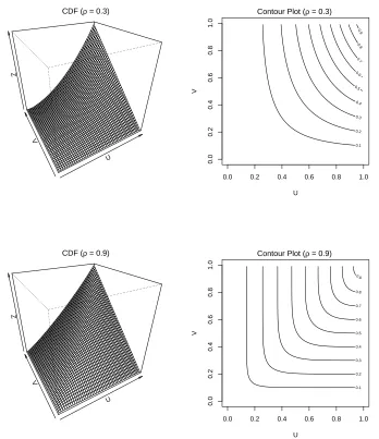
Examples of the Gaussian copula for different correlation coefficientsρ= 0.3 and 0.9
are given in Figure 2.3.3. As ρ → 0 the Gaussian copula resembles the independence
copula in Figure 2.3.1, whilst as ρ → 1 it resembles the perfect dependence copula of
Figure 2.3.2.
The symmetry illustrated in these contour plots is a key property of this model (as
U
V Z
CDF (ρ = 0.3)
U V 0.1 0.2 0.3 0.4 0.5 0.6 0.7 0.8 0.9
0.0 0.2 0.4 0.6 0.8 1.0
0.0 0.2 0.4 0.6 0.8 1.0
Contour Plot (ρ = 0.3)
U
V Z
CDF (ρ = 0.9)
U V 0.1 0.2 0.3 0.4 0.5 0.6 0.7 0.8 0.9
0.0 0.2 0.4 0.6 0.8 1.0
0.0 0.2 0.4 0.6 0.8 1.0
[image:39.612.145.493.94.497.2]Contour Plot (ρ = 0.9)
Figure 2.3.3: Surface and contour plots of the cumulative distribution function for the Gaussian dependence copula
and Y are interchangeable.
The extreme value copula class
Extreme-value copulas characterise the dependence structure between suitably
nor-malised component-wise maxima. They are of particular interest in insurance and
man-agement of risk. This interest is common to our motivating service industry problem,
in which joint high demand for skills puts strain on the availability of human resources,
increasing the risk of fines or damaged reputation.
To define this copula class we first need to characterise univariate variation in the
maxima of sequences of i.i.d. random variables via definition of the generalised extreme
value distribution.
Univariate Extreme Value Distributions
Let X1, . . . , Xn be independent and identically distributed random variables with
distribution function FX(·), and let MX,n = max(X1, . . . , Xn) define their
component-wise maxima. If there exist sequences{an}>0 and {bn} of normalising constants such
that
P{(MX,n−bn)/an≤z}=Fn(anz+bn)
converges in distribution to a non-degenerate distribution G as n → ∞, then G must
necessarily be the generalised extreme value (GEV) distribution. This distribution
sum-marises three distributions originally identified by Fisher and Tippett (1928), namely
the Fr´echet, Weibull and Gumbel distributions and has distribution function
G(z;µ, σ, k) = exp
"
−
1−k
z−µ σ
1/k# ,
whereσ >0 and the range ofz follows from 1−k(z−µ)/σ >0. The Fr´echet distribution
arises when k < 0, the Gumbel distribution when k = 0 and the Weibull distribution
whenk > 0.
The unit Fr´echet distribution, with cumulative distribution functionF(z) = exp(−1/z),
in the presentation of theory relating to extreme values without loss of generality. We
follow this convention in the following introduction to the extreme value copula class.
Multivariate Extreme Value Distributions
Suppose that (Xi, Yi)i=1:n defines an independent and identically distributed series
of random vectors with unit Fr´echet margins, and define the vector of componentwise
maxima asMn ={MX,n, MY,n} (where MY,n is similarly defined to MX,n above).
Sub-ject to weak regularity conditions, the limiting distribution of n−1Mn has distribution
function
P(MX,n/n≤x, MY,n/n≤y) = {F(nx, ny)}n →G(x, y),
asn → ∞, where G(x, y) is non-degenerate and can be written in the form
G(x, y) = exp{−V(x, y)}. Exponent measureV(·) summarises the extremal dependence
structure and provided that
V(x, y) =
Z 1 0
max
w
x,
1−w y
2dH(w)
for some distribution function H on [0,1] satisfying moment constraint
Z 1
0
wdH(w) = 1/2,
distribution function G(x, y) belongs to the bivariate extreme value class (Coles et al.
(1999)).
distri-butions, arises when
Vα(x, y) = x−1/α+y−1/α
α , and
Hα(w) =
1 2
h
w(1−α)/α−(1−w)(1−α)/α
w1/α+ (1−w)1/α α−1+ 1i,
for parameter 0 < α ≤ 1 which controls the strength of extremal dependence. The
joint distribution function for this bivariate logistic extreme value class, on unit Fr´echet
marginsFX(·) and FY(·), is given by
FX,Y(x, y) = P(X ≤x, Y ≤y) = exp
− x−1/α+y−1/α,
for x >0, y > 0 and α ∈(0,1). Noting that the inverse of the cumulative distribution
function for the unit Fr´echet distribution is given by FX−1(u) = −log (u)−1, we can pull out the definition of the bivariate logistic extreme value copula on uniform margins:
C(u, v) =FX,Y FX−1(u), F
−1
Y (v)
C(u, v) =FX,Y −log(u)−1,−log(v)−1
C(u, v) = exph−n(−log u)1/α+ (−log v)1/αo
αi
. (2.3.5)
The strength of extremal dependence is governed by parameterα ∈(0,1], where α= 1
defines independence and α → 0 leads to increasing dependence up to perfect
depen-dence in the limit. This model shares the symmetry of the Gaussian copula model, with
variablesX and Y again interchangeable.
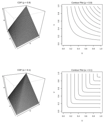
The cumulative distribution function, illustrated in Figure 2.3.4, does not appear
markedly different to that of the Gaussian copula in Figure 2.3.3. The key difference
between these copula families is in their modelling of extremal dependence, and so a
value for V given a large value of U. We explore summary measures for this domain in
the following subsection.
U
V Z
CDF (ρ = 0.9)
U V 0.1 0.2 0.3 0.4 0.5 0.6 0.7 0.8 0.9
0.0 0.2 0.4 0.6 0.8 1.0
0.0 0.2 0.4 0.6 0.8 1.0
Contour Plot (ρ = 0.9)
U
V Z
CDF (α = 0.1)
U V 0.1 0.2 0.3 0.4 0.5 0.6 0.7 0.8 0.9
0.0 0.2 0.4 0.6 0.8 1.0
0.0 0.2 0.4 0.6 0.8 1.0
[image:43.612.144.489.148.550.2]Contour Plot (α = 0.1)
Figure 2.3.4: Surface and contour plots of the cumulative distribution function for the logistic extreme value copula
2.3.3
Extremal Dependence
It is often useful to be able to reduce the information in the copula to a single summary
can aid inference and ease interpretation of multi-dimensional dependence. As the
simultaneous occurrence of high demand in multiple skills is of particular relevance in
cross-trained workforce planning, we consider two closely related measures of extremal
dependence.
A natural measure of extremal dependence between non-identically distributed pairs
of variables (X, Y) is given by transforming onto uniform margins (U, V) and measuring
χ∗ = lim
u→1P(V > u|U > u) = limu→1
P(U > u, V > u)
P(U > u)
, (2.3.6)
the probability of one variable being extreme when the other is extreme. When χ∗ =
0, the largest values of U and V are unlikely to occur simultaneously and so U and
V are said to be asymptotically independent. The complementary case of asymptotic dependence follows from χ∗ = 1.
We can obtain measure χ∗ as the limit as u→ ∞ of one of the following functions
described in Coles et al. (1999)
χ(u) =P(V > u|U > u)
= P(V > u, U > u)
P(U > u)
= 1−2u+C(u, u) 1−u
= 2− 1−C(u, u)
1−u ; or (2.3.7)
χl(u) = 2−
log C(u, u)
log u . (2.3.8)
Function χl(u) is asymptotically equivalent to χ(u), with χl(u) ∼ χ(u) as u → 1, but
has different properties foru <1.
χl(u) provide their own useful insights since they can be interpreted as quantile-dependent
measures of dependence. In particular,χl(u) is constant inufor three of the four copula
families introduced in Section 2.3.2 (all except for the Gaussian copula). Specifically,
for independent variablesχl(u) = 0 and for perfectly dependent variablesχl(u) = 1. In
the case of the bivariate logistic extreme value distribution
χl(u) = 2−
log C(u, u) log u
= 2−
log exph−n(−log u)1/α+ (−log u)1/αoαi log u
= 2−
−n2 (−log u)1/αo
α
log u
= 2 + {2
α(−log u)}
log u
= 2−2α
so that there is a clear relationship between extremal dependence measure χl(u) and
the extremal dependence parameter α specifying the distribution itself. Plots of
em-pirical estimates of χl(u) can therefore provide a useful diagnostic for the membership
or otherwise of a pair of variables to these copula models via a simple by-eye check of
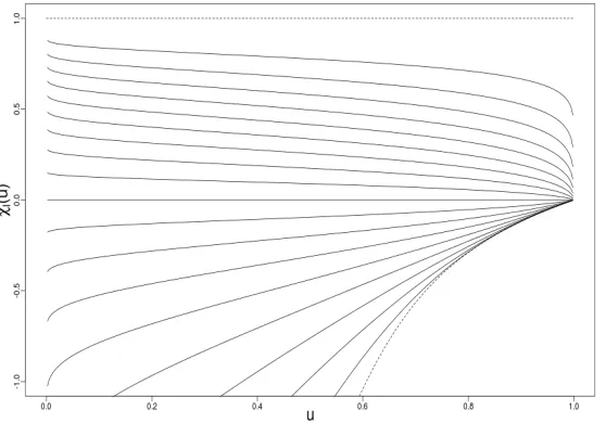
constancy. Figure 2.3.5 illustratesχl(u) for a range of values of α with the upper-most
line corresponding to α = 0.1, and lines at lower levels corresponding to α ∈ [0.2,0.9]
in increments of 0.1. The upper and lower bounds ofχl(u) are given as dotted lines.
For the Gaussian dependence model, χl(u) is a considerably less trivial function
when its dependence parameter, correlation coefficient ρ, is non-zero. In such cases
χl(u) is non-constant inuand its evaluation requires numerical integration. Figure 2.3.6
demonstrates this function for a range of correlation coefficients ρ. The sign of χl(u)
immediately tells us whether the association between variables is positive or negative,
Figure 2.3.5: Extremal dependence measure χl(u) for the bivariate logistic extreme value
copula: solid lines (bottom to top) correspond to α = 0.9,0.8, . . . ,0.1 and dashed lines give the bounds ofχl(u)
ρ ∈ [−0.8,0.9] in increments of 0.1. Again, the upper and lower bounds of χl(u) are
given as dotted lines.
Figure 2.3.6: Extremal dependence measure χl(u) for the bivariate Gaussian copula: solid
curves (bottom to top) correspond to correlation coefficientρ=−0.9,−0.8, . . . ,0.9 and dashed curves give the bounds ofχl(u).
In contrast to the extremal dependence functions for the perfect dependence and
decreases, i.e. χl(u)→0 for allρ <1. The very slow convergence forρ >0, resulting in
an sudden drop to 0 whenuis very close to 1, is of practical importance since empirical
estimates ofχl(u) may appear constant and non-zero (suggesting perfect dependence or
bivariate logistic extreme dependence) even for asymptotically independent variables.
We therefore take caution in this respect when diagnosing membership of bivariate data
to these copula models.
2.4
Stochastic Linear Programming
In this section we introduce techniques for finding the best possible decisions given some
criteria expressed in the form of an objective function and constraints. Coordinating
the work of a hand-full of individuals is a complex task with time-off, different working
patterns and skills to consider amongst many other factors. Though this task is possible
and perhaps even best performed by a manager on a small scale, the explosion in the
complexity of the problem as the number of workers increases means it soon becomes
a combinatorial task too large for a single person to compute without the help of a
computer. Planning on a scale of tens of thousands of individuals soon benefits from
automated systems which can capture basic desirable outcomes (e.g. balancing supply to
meet demand within normal working hours) and optimise over the thousands of possible
deployments of the workforce.
We begin by describing the formulation of decision problems as mathematical
pro-grams with the simplest case: deterministic linear propro-grams. Following this, we evaluate
how this theory stands up when certain input data is uncertain. This motivates an
2.4.1
Decision Problems as Linear Programs
Linear programs express decision problems as a mathematical model in which
require-ments are represented by a linear objective function and linear equality and inequality
constraints. In vector-matrix notation, linear programs take the following form:
min cTx,
s.t. Ax ≤b,
x ≥0;
wherexis an (n×1) vector of decisions andc, band Aare known data of sizes (n×1), (m×1) and (m×n) respectively. This data might represent demand counts, supply
levels, productivity measures and so on. The quantity we wish to minimise with respect
to the decisionxis captured using objective functioncTxwhich might summarise total costs or, say, incomplete work over a planning horizon. An optimal solution to the linear
program, x∗, must belong to the feasible set of decisions F ={x∈Rn|Ax≤b,x≥0}
and satisfy
cTx≥cTx∗ for all x∈ F \x∗.
Since their introduction by George B. Dantzig in 1947, linear programs have been
extensively applied to practical decision problems. With extensions to integer decision
variables and the use of non-linear functions in the objective and constraints, a more
general class ofmathematical programs emerged:
min f(x),
s.t. gi(x) =bi, fori∈ {1, . . . , m}
x ∈Rn,
and hence benefit from being modelled as a non-linear program in which some or all functionsf andgi are non-linear. Examples include economies of scale in manufacturing
or the drop in signal strength with distance from a transmitter.
Certain functional forms for f and gi, due to their role in model formulation and
convenient mathematical properties, are predominant in mathematical programming.
Linear functions are by far the most applicable in formulation and define linear programs
which are particularly easy to solve. More generally, linear programs have the advantage
of belonging to an important class of convex optimisation problems in which f and gi
(fori∈ {1, . . . , m}) are convex functions and the feasible region is aconvex set. A real valued function f(x) defined over points (x1, . . . , xn) is said to be a convex function if
and only if for any two pointsx= (x1, . . . , xn) and y= (y1, . . . , yn),
f(λx+ (1−λ)y)≤λf(x) + (1−λ)f(y)
for allλ∈[0,1]. When the inequality is strict, the function is said to be strictly convex
(Dantzig and Thapa, 1997). The feasible region of a non-linear program is aconvex set provided it is specified by less-than-or-equal-to constraints involving convex functions.
Convex optimisation problems benefit from the guarantee that every local minimum
so-lution is in fact a global minimum. This property renders convex optimisation problems
considerably easier and faster to solve than their non-convex counterparts.
Another important consideration when formulating mathematical programs which
can be solved quickly, is the requirement or otherwise for some or all decision variables to
be integers. The associated class ofinteger programs are generally much harder to solve. Roughly speaking, the efficient solution methods used to search the single continuous
and convex solution space (present in continuous convex optimisation problems) cannot
2.4.2
Stochastic Linear Programming
In the optimisation problems discussed above, all inputs were assumed to be
determin-istic in nature. In many real problems however, it is not reasonable to assume that problem parametersc, A,b,gi are deterministically known. The future productivity of
a worker or the demand experienced at different points in time, for example, are better
modelled by random variables and hence best characterised by probability distributions
(King and Wallace, 2012).
The aim of Stochastic Programming is to find optimal decisions for problems which
involve uncertain data. Uncertainty can be represented in terms of random experiments
with outcomesω. The values that the various random variables take, denoted by vector
ξ, are known only after the random experiment so that ξ =ξ(ω).
Models in which some decisions are delayed until after information about uncertain
quantities has been disclosed are referred to as recourse problems and form a powerful area of stochastic programming.
We can recognise decisions as falling into two groups (Birge and Louveaux, 1997):
1. First-stage decisions which have to be made before the experiment or before the uncertain information is realised and available; and
2. Second-stage decisions which can be made after the experiment.
In general recourse program notation,xtraditionally represents first stage decisions and
y(ω,x) the second stage decisions. We summarise the sequence of events with
x→ξ(ω)→y(ω,x).
Dantzig (1955) and Beale (1955), is then the problem defined by
min cTx+Eξ[min q(ω)Ty(ω,x)],
s.t. Ax=b,
T(ω)x+W(ω)y(ω,x) = h(ω),
x,y(ω,x)≥0. (2.4.1)
Our first-stage or here-and-now decision x does not respond to the outcome of ξ
in any way since it is determined before any information relating to uncertain data
has become available. Associated with the first stage problem are the vectors c, b and matrix A.
In the second stage, any random event (from a set of possible events Ω) may be
realised. For a given realisation ω, the problem data q(ω), h(ω), T(ω) and W(ω) become known, at which point the second stage decision y(ω,x) must be made. By definition, the single random eventω influences several random variables, here they are every component of ξ.
We can understand the goal of such models as identifying a first stage solution
well-positioned against all possible outcomes in the second stage so that advantageous
outcomes of ξ can be exploited without major vulnerability to disadvantageous ones. The objective function contains both a deterministic term cTx and the expectation
of the second stage objectiveq(ω)Ty(ω,x) taken over all realisations ofξ. This second
stage term is the more difficult to compute since for eachω, y(ω,x) is the solution to a linear program in itself. To be able to solve stochastic programs, we therefore need
to be able to effectively discretise the continuous distribution of stochastic variablesξ, summarising it using a finite set of samples or ‘scenarios’. We wish to discretise the
distribution. This discretisation problem is discussed in more detail in the following
subsection.
Discretisation of the expectation forming the second-stage sub-problem allows us to
define thedeterministic equivalent linear programassociated with the original continuous problem. This notion is sometimes used to stress and clarify the ‘program within a
program’ structure of model (2.4.1).
Defining the second stage value function for a given realisation ω as
Q(x,ξ(ω)) = min y{q(ω)Ty(ω,x)|W(ω)y(ω,x) =h(ω)−T(ω)x,y(ω,x)≥0},
the expected second stage value function, defined over discrete scenario set S, is thus defined as
Q(x) =X
s∈S
psQ(x,ξ(ω)),
whereps ∈[0,1] is the probability associated with each scenario s∈S.
We then have the so-called deterministic equivalent program
min cTx+Q(x) s.t. Ax=b,
x≥0. (2.4.2)
This model’s name gives away the fact that it is essentially one very large-scale
ver-sion of a standard deterministic linear program and writing it in this form opens up a
range of decomposition based solution techniques which exploit its underlying structure.
Indeed we can solve increasingly large two-stage deterministic equivalent programs
us-ing a variant of Dantzig-Wolfe Decomposition (or Column Generation) called Benders
(1997).
Two-stage stochastic programs can be extended to multiple stages with a simple
amendment of the linear program above. The additional decision stages result in a
scenario tree which quickly explodes in size however. Despite the progress made in
solving two-stage stochastic programs, multi-stage programs remain elusively difficult
to solve for more than a few stages of decision making and a hand-full of scenarios.
2.4.3
Scenario Generation
There are numerous approaches to finding a representative discrete scenario set for the
second-stage sub-problem. Indeed a category of literature called scenario generation dedicates itself to this problem.
The key goal of the scenario generation procedure is for it to be unobservable in the
solution of the model. The discretised model should function as it would have had the
whole distribution been used. That is, we want the model (the algebraic formulation
and decision variables) to drive the optimisation problem and not the discretisation
procedure.
Kaut and Wallace (2007) identify two useful properties in the evaluation of scenario
generation procedures:
• In-sample stability: a test for the robustness of the discretisation procedure, it ensures that the optimal objective function value is roughly the same for any
scenario-tree generated by the (random) scenario generation procedure; and
• Out-of-Sample Stability: ensures that the true objective function value correspond-ing to solutions resultcorrespond-ing from different scenario trees are roughly equal.
Let Si and Sj represent two scenario trees resulting from two different runs of a