a s e l f - c o n ta i n e d g r o u n d - s tat e
a p p r o a c h f o r t h e c o r r e c t i o n o f
s e l f - i n t e r a c t i o n e r r o r i n
a p p r o x i m at e d e n s i t y - f u n c t i o n a l
t h e o ry
Glenn Moynihan
t h e u n i v e r s i t y o f d u b l i n t r i n i t y c o l l e g e
a d i s s e rtat i o n s u b m i t t e d f o r
t h e d e g r e e o f d o c t o r o f p h i l o s o p h y at t h e u n i v e r s i t y o f d u b l i n
d e c l a r at i o n
I
d e c l a r ethat this thesis has not been submitted as an exercise for a degree atthis or any other university and it is entirely my own work. I agree to deposit this
thesis in the University’s open access institutional repository or allow the Library
to do so on my behalf, subject to Irish Copyright Legislation and Trinity College
Library conditions of use and acknowledgement. Except where otherwise stated, the
contents of this thesis are the product of my own work carried out in the Condensed
Matter Theory group at the School of Physics, Trinity College Dublin, supervised
by Professor David D. O’Regan.
This dissertation does not exceed 60,000 words in length.
Glenn Moynihan
Trinity College Dublin
s u m m a ry
D
e n s i t y - f u n c t i o n a l t h e o ry(DFT), in its approximate Kohn-Shamformalism, is a highly-acclaimed computational tool that affords the
prac-tical and expeditious calculation of ground-state properties of molecules and solids,
often with a very reasonable accuracy. It finds routine application in the fields of
chemistry, physics, materials science, and biochemistry, where it now contributes in
both a descriptive and predictive capacity.
It is not, in practice, without systematic errors such as those defined by
self-interaction and static correlation. These errors undermine the accurate description of
particular systems that are beyond the scope of the approximate exchange-correlation
functionals, particularly for those comprising so-calledstrongly-correlated electrons.
The effective treatment of these errors is laid down in a number of formative works
now adopted within the canon of Kohn-Sham DFT. Many of the most popular and
affordable correction schemes entail the calculation of external parameters to diagnose
and treat these pervasive errors on a per-electron basis, such as the DFT+Hubbard
U method.
A possibility that has not yet been explored, however, is the automation of these
correction schemes for the provision of greater efficiency, versatility and
comparabil-ity between DFT calculations. An automated procedure would enable the correction
process to be self-contained, thereby circumventing the need for human input, and
es-tablish a standardised approach between the various softwares and electronic systems.
Of particular interest is the application in high-throughput materials design, and
the comparability of DFT+U total-energies for the calculation of thermodynamical quantities.
In this dissertation, we present a comprehensive account of our work in pursuit of
this goal. We motivate and describe an efficient self-contained approach for correcting
the many-body self-interaction error in strongly-correlated systems from ground-state
Specifically, we develop a highly accurate variational linear-response approach for
calculating the HubbardU and Hund’s J parameters, for which a unique criterion for their self-consistency is identified. Our results demonstrate that this scheme is
accurate and versatile, and facilitates the correction of many-body self-interaction
error for various systems. Moreover, we propose the novel construction of a generalised
DFT+U functional that resolves Koopmans’ condition exactly in a one-electron system when supplied with the appropriate self-consistentU value.
Our research provides insight into important questions about the practice and
con-sequences of calculating corrective parameters for approximate DFT self-consistently,
a c k n o w l e d g m e n t s
T
h e w o r k d e s c r i b e din this dissertation could not have been completedwithout the assistance and support from various people and institutions over
the years, and it is a pleasure to take this opportunity to pay tribute to those who
have aided in its completion.
I would first like to thank Science Foundation Ireland for providing the funding for
this research through the A M B E R program, as well as the Royal Irish Academy for facilitating the project collaboration with our colleagues at the University of
Liverpool. I also wish to thank Trinity College for their generous support through
the provision of the Non-Foundation Scholarship. I am grateful to the staff at the
School of Physics for their assistance over the years, and to Trinity Research IT
and I C H E C for providing computing resources, as well as the C R A N N and
A M B E R support staff.
Much of this work would not be possible were it not for my esteemed colleagues.
I would like to thank the members of the Computational Spintronics Group for their
constructive feedback and discussions when presented with my work. I am deeply
grateful in particular to my co-supervisor, Professor Stefano Sanvito, for all of his
valuable help and guidance in my studies.
The members of the Chemical Physics of Low-Dimensional Nanostructures Group,
Professor Johnny Coleman, Dr Damien Hanlon, Dr Conor Boland, and Dr Claudia
Backes deserve a special thanks for expediting my first publication. I am grateful
also to Emma Norton and Dr Karsten Fleischer of the Applied Physics Research
Group for their helpful discussions and for contributing their experimental data. I also
appreciate the helpful discussions with Fiona McCarthy, Mark McGrath, Thomas
Wyse Jackson, and Edward Linscott.
The members of the O N E T E P community were very helpful to me during the
coding retreats. I appreciate their assistance very much.
My time in Dublin was frequently punctuated by visits to the University of
arrival. I would therefore like to extend my warmest appreciation to the venerable Dr
Gilberto Teobaldi for making each of these visits an absolute pleasure, even on those
dark December days. His valuable assistance, inexhaustible patience, and excellent
taste in hotels aided my stay immeasurably. Many thanks + cheer up.
I would like to give a special mention to my office-mates, who I have had the
utmost pleasure of working beside: Dr James Lawlor, Dr Eric Mehes, Dr Pankaj
Kumar, Dr Alessandro Lungi, Dr Claudia Rocha, Dr Linda Zotti, and last, but
certainly not least, Okan Karaca Orhan. You have each made a valuable contribution
to my postgraduate experience. I thank you all for the welcome distractions.
It would be remiss of me to fail to mention my distinguished flatmates, Izzy
Kennedy, Lauren Boland, Naomi Beard and Niamh Ennis, whose company was the
highlight of my years living on Trinity College campus.
I would like to extend my heartfelt gratitude to my supervisor, Professor David
O’Regan, to whom I am truly indebted most of all, not least for taking a fellow
Corkman under his wing. I have been extremely fortunate to be under his considerate
mentorship the last four years. His continuous encouragement, attentive guidance,
and meticulous work ethic are an example to aspire to.
I am especially privileged to have had Olivia Kerrigan by my side the last few
years. I can only hope to repay the patience and devotion she has afforded me during
these months of writing. She continues to brighten the otherwise anarchic days of
the Ph.D. experience. I also humbly thank the Kerrigan family for graciously hosting
me for the final push.
Finally, I would to thank my friends and family who have made my time here in
Dublin over the past eight years very special. In particular, my parents, Karen and
Michael, grandparents, and siblings who have all supported me relentlessly in the
l i s t o f f i g u r e s
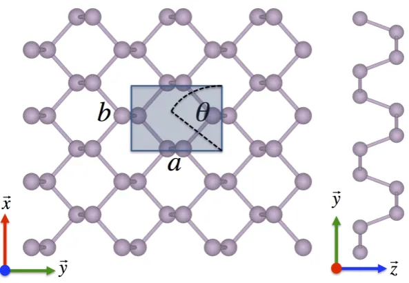
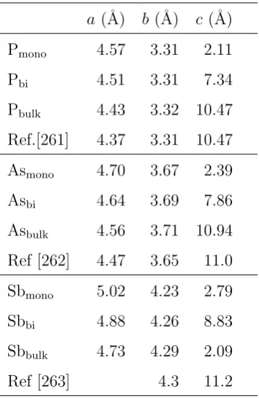
III.1 Crystal structure of orthorhombic black phosphorus . . . 37
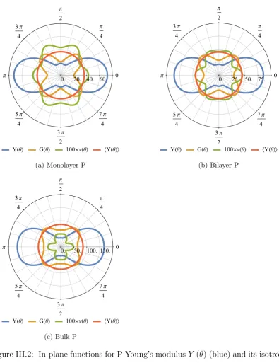
III.2 Phosphorus in-plane mechanical properties . . . 46
III.3 Arsenic in-plane mechanical properties . . . 47
III.4 Antimony in-plane mechanical properties . . . 48
III.5 PVC:BP Young’s modulus fit to rule-of-mixtures model . . . 50
III.6 PVC:BP Young’s modulus fit to Halpin-Tsai model . . . 51
IV.1 Brillouin zone of orthorhombic phosphorus . . . 55
IV.2 Electronic properties of monolayer phosphorus for in-plane strains . 57 IV.3 Electronic properties of bilayer phosphorus for in-plane strains . . . 58
IV.4 Predicted Dirac states of strained bilayer phosphorus . . . 59
IV.5 Electronic properties of bulk phosphorus for in-plane strains . . . . 61
IV.6 Predicted Weyl states of strained bulk phosphorus . . . 62
IV.7 Electronic properties of monolayer arsenic for in-plane strains . . . 63
IV.8 Predicted Dirac states of strained monolayer arsenic . . . 64
IV.9 Electronic properties of bilayer arsenic for in-plane strains . . . 65
IV.10 Predicted Dirac states of strained bilayer arsenic . . . 66
IV.11 Electronic properties of bulk arsenic for in-plane strains . . . 67
IV.12 Predicted Weyl states of strained bulk arsenic . . . 68
IV.13 Electronic properties of monolayer antimony for in-plane strains . . 69
IV.14 Predicted Dirac states of monolayer antimony . . . 70
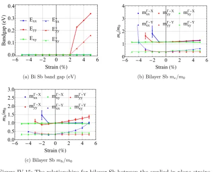
IV.15 Electronic properties of antimony for in-plane strains . . . 71
IV.16 Predicted Dirac states of bilayer antimony . . . 72
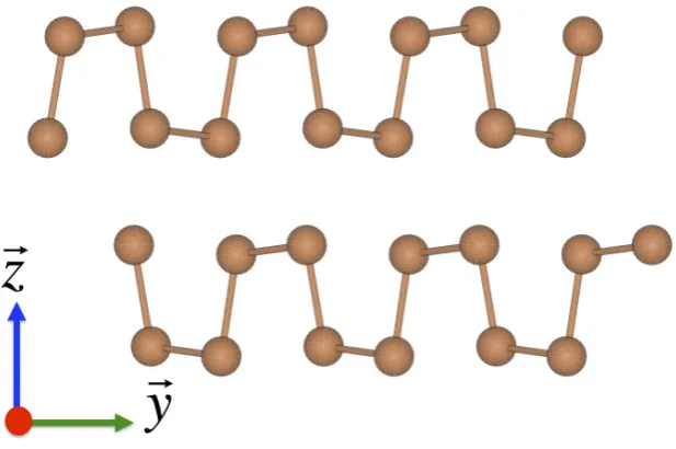
IV.17 Strain-induced buckled phase in bilayer antimony . . . 72
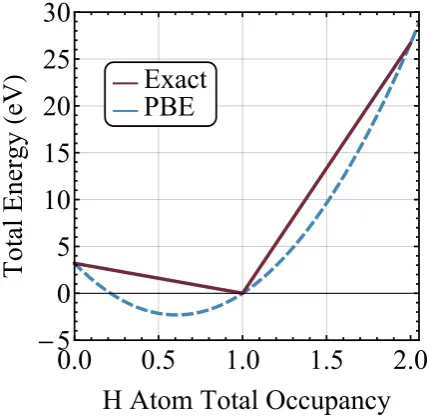
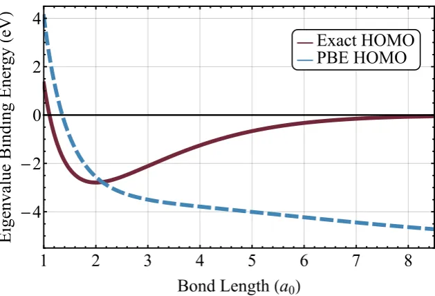
V.1 SIE of a H atom as the deviation from piece-wise linearity . . . 77
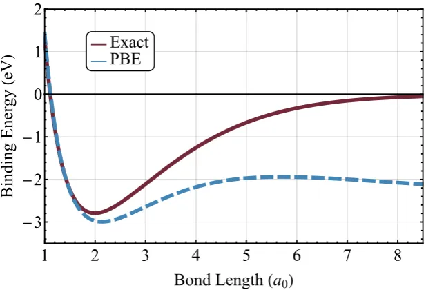
V.2 Binding energy curve of H+2 . . . 78
V.3 Occupancy of H atom in dissociating H+2 . . . 79
l i s t o f f i g u r e s
V.5 Binding energy curve of H+2 with DFT+U . . . 89
V.6 Eigenvalue-derived binding energy of H+2 with DFT+U . . . 90
V.7 Binding energy curve of H2 with DFT+U . . . 92
V.8 SCE of a H2 molecule as the deviation from piece-wise constancy . 95 V.9 Binding energy curve of H2 with DFT+J . . . 96
VI.1 Variational linear-response U values calculated for dissociating H+2 . 112 VI.2 PBE+U binding curve of H+2 with linear-response U . . . 113
VI.3 PBE+U binding curve of H2 with linear-response U . . . 114
VI.4 Ni(CO)4 molecular structure and linear-response calculation . . . . 116
VI.5 NiO crystal structure and linear-response calculation . . . 117
VI.6 Species-resolved DOS for NiO calculated with PBE . . . 118
VI.7 Species-resolved DOS for NiO calculated with PBE+U . . . 119
VI.8 Cr2O3 crystal structure and linear-response calculation . . . 120
VI.9 Species-resolved DOS for Cr2O3 calculated with LDA . . . 122
VI.10 Species-resolved DOS for Cr2O3 calculated with LDA+U . . . 123
VI.11 Normalised XPS and UPS measurements of Cr2O3 compared to LDA+U total DOS . . . 124
VI.12 Normalised XPS and UPS measurements of Cr2O3 compared to LDA+U species-resolved DOS . . . 125
VI.13 Normalised absorption spectrum of Cr2O3 compared to LDA+U joint DOS . . . 126
VI.14 Stable and unstable magnetic potentials for H2 at 1 a0 and 4.8 a0 bond-length . . . 130
VI.15 Species-resolved DOS for NiO calculated with PBE+U+J . . . 132
VI.16 Species-resolved DOS for Cr2O3 calculated with PBE+U+J . . . . 132
VII.1 Example of Uin vs Uout profile for H+2 . . . 142
VII.2 Self-consistent Uout schemes for H+2 vs best estimated U . . . 145
VII.3 Binding energy of H+2 calculated with various Uout schemes . . . 146
VII.4 Profiles of Uout, Jout,Ueff vs Uin for NiO . . . 153
Chapter
VII.6 Ranking of all self-consistency schemes for NiO . . . 158
VII.7 NiO DOS with U = 4.1 eV andJ = 0 eV . . . 160
VII.8 NiO DOS with U = 10.5 eV andJ = 0 eV . . . 161
VII.9 NiO DOS with U = 6.7 eV andJ = 0.84 eV . . . 162
VII.10 NiO DOS with Ueff= 5.2 eV . . . 163
VII.11 Jin vs Jout calculations for H2 at 1 a0 and 6 a0 bond-length . . . 165
VII.12 Calculated Jout schemes for dissociating H2 . . . 166
VII.13 Binding energy of H2 with PBE+J(2) . . . 167
VII.14 The self-consistent U profile for H2 at 2.8 a0 . . . 168
VII.15 Approximated Ueff and Jeff for dissociating H2 . . . 169
VIII.1 Total-energy of constrained H+2 vs Lagrange multiplier . . . 178
VIII.2 Interacting response functions for H+2 vs Lagrange multiplier . . . . 179
VIII.3 Constraint energy landscape of H+2 vs Lagrange multipliersU1 and U2185 VIII.4 DFT+U1+U2 free energy landscape of H+2 . . . 188
VIII.5 EstimatedU1 and U2 parameters to restore exact total-energy and Koopmans’ condition in dissociating H+2 . . . 189
VIII.6 Total-energy and eigenvalue binding curves for H+2 calculated with generalised DFT+U functional . . . 192
B.1 Band structures of relaxed group-V phases . . . 216
C.1 NiO DOS with U = 4.1 eV andJ = 2.82 . . . 219
C.2 NiO DOS with U = 10.5 eV andJ = 5.9 . . . 219
C.3 NiO DOS with U = 4.1 eV andFJ = 0.78 . . . 220
C.4 NiO DOS with U = 10.5 eV andFJ = 0.69 . . . 220
C.5 NiO DOS with U−J = 1.3 eV . . . 221
C.6 NiO DOS with U−J = 4.6 eV . . . 221
C.7 NiO DOS with U−J = 5.9 eV . . . 222
C.8 NiO DOS with Ueff= 5.2 andJ = 3.48 eV . . . 222
C.9 NiO DOS with Ueff= 5.2 andFJ = 0.84 eV . . . 223
l i s t o f f i g u r e s
C.11 Self-consistency profile for Ni(CO)4 . . . 224
C.12 Self-consistency profile for Cr2O3 . . . 225
ta b l e o f c o n t e n t s
d e c l a r at i o n i
s u m m a ry iii
a c k n o w l e d g m e n t s v
l i s t o f f i g u r e s vii
I i n t r o d u c t i o n 1
1 Outline of dissertation . . . 3
2 Associated publications . . . 6
II q u a n t u m m e c h a n i c a l s i m u l at i o n 7 1 The Schr¨odinger equation . . . 8
2 The Hohenberg-Kohn theorems . . . 9
3 The Kohn-Sham equations . . . 13
4 Exchange-correlation functionals . . . 16
5 Treatment of the ionic potential . . . 18
5.1 Norm-conserving pseudopotentials . . . 18
5.2 Projector-augmented wave method . . . 21
6 An overview of linear-scaling DFT . . . 24
6.1 Density matrix formalism in DFT . . . 25
6.2 Psinc basis sets . . . 26
6.3 Non-orthogonal generalised Wannier functions . . . 27
6.4 Brillouin zone sampling in O N E T E P . . . 30
7 Conclusion . . . 32
ta b l e o f c o n t e n t s
2 Methodology . . . 38
2.1 Calculation details . . . 38
2.2 The Voigt-Reuss-Hill scheme . . . 39
2.3 In-plane Voigt-Reuss-Hill average . . . 40
2.4 Composite mixture models . . . 40
3 Results . . . 42
3.1 Calculated lattice constants . . . 42
3.2 Isotropic bulk properties . . . 43
3.3 In-plane elastic properties . . . 44
3.4 Polymer-nano-flake composite . . . 49
4 Conclusion . . . 52
IV e l e c t r o n i c p r o p e rt i e s o f t w o - d i m e n s i o n a l g r o u p - V m at e r i a l s 53 1 Weyl and Dirac semi-metals . . . 54
2 Methodology . . . 54
3 Electronic properties . . . 56
4 Conclusion . . . 70
V t h e n at u r e a n d o r i g i n o f p e rva s i v e e r r o r s i n a p p r o x i m at e D F T 75 1 Fractional charges . . . 76
2 One-electron self-interaction correction . . . 79
3 Koopmans’ compliance . . . 80
4 Strongly correlated systems . . . 83
5 The DFT+U method . . . 84
5.1 A one-electron assessment of DFT+U . . . 88
6 Static Correlation Error . . . 91
Chapter
VI c a l c u l at i o n o f h u b b a r d pa r a m e t e r s f r o m
va r i at i o n a l l i n e a r r e s p o n s e 99
1 Overview of the linear-response method . . . 100
2 Construction of a variational linear-response approach . . . 102
2.1 The non-interacting response . . . 103
2.2 Choice of projection for the interacting kernel . . . 104
2.3 Comparing the SCF and variational linear-response methods . . . 108
2.4 The subspace contribution to SIE: global vs local curvatures . . . 109
2.5 A one-electron test case: H+2 . . . 111
3 Application to multi-electronic systems . . . 113
3.1 Dissociating H2 . . . 113
3.2 Molecular Ni(CO)4 . . . 114
3.3 Bulk NiO . . . 115
3.4 Bulk Cr2O3 . . . 119
4 Calculating J using the variational linear-response method . . . 126
4.1 Correcting static correlation error in H2 . . . 128
4.2 Calculating J for NiO and Cr2O3 . . . 130
5 Conclusion . . . 134
VII c a l c u l at i o n o f s e l f - c o n s i s t e n t h u b b a r d pa r a m e t e r s 137 1 A note on the direct comparison of DFT+U total-energies . . . 139
2 A self-consistent U in a one-electron model . . . 140
2.1 Which self-consistency scheme?: revisiting H+2 . . . 143
3 Coupled self-consistent parameters in multi-electronic systems . . . . 148
3.1 Generalised, self-consistent U and J formulae . . . 149
3.2 Application to NiO . . . 152
3.3 Comparison of self-consistency schemes . . . 159
4 A self-consistent J applied to H2 . . . 164
4.1 Correcting SCE with J . . . 165
ta b l e o f c o n t e n t s
5 Choice of subspace projectors . . . 169
6 Conclusion . . . 171
VIII t h e i n v e s t i g at i o n o f n o n - l i n e a r c o n s t r a i n t s a n d a g e n e r a l i s e d D F T + U f u n c t i o n a l 173 1 Constrained-DFT . . . 175
2 Non-linear constraints . . . 176
2.1 Proof of the inapplicability of non-linear constraints . . . 179
2.2 Construction of separable constraints . . . 183
3 A generalised DFT+U formula . . . 186
3.1 Non-self-consistent estimates for U1 and U2 . . . 188
3.2 Application to H+2 . . . 191
4 Conclusion . . . 192
IX c o n c l u d i n g r e m a r k s 195 1 Synopsis . . . 195
2 Future work . . . 199
A Sample input files 203 1 Sample Q u a n t u m E s p r e s s o input file . . . 203
2 Sample O N E T E P input file . . . 204
B Supplemental data for group-V 2D materials 208 1 Deriviation of the Voigt-Reuss-Hill Equations . . . 208
2 Calculated elastic tensor elements . . . 211
3 Group-V in-plane elastic extrema . . . 212
4 Black phosphorus experimental data . . . 213
5 Summary of electronic properties . . . 214
6 Summary of electronic transitions . . . 215
7 Band structures figures . . . 216
Chapter
2 Supplemental DOS plots for NiO . . . 219
2.1 Self-consistency calculations for Ni(CO)4 . . . 224
I
i n t r o d u c t i o n
All models are wrong but some are useful.
George E. P. Box [1]
T
h e p i l l a r s o f m o d e r n physics now comprise the well establishedfields of theory, experiment and simulation, where the latter addition has been
made possible thanks to the technological advances of the 20thcentury, characterised
by Moore’s law [2]. In the current ‘Age of Silicon’ [3] simulation and modelling have
become indispensable tools that find cutting-edge application in the field of quantum
physics, in particular for solving the complex many-body Sch¨odinger equation [4].
Notwithstanding the significant progress made in micro-processors over the last five
decades, it is only by the intelligent use of algorithms and suitable approximations
that it is possible to quantitatively describe chemical processes and complex material
properties with sufficient accuracy and efficiency.
Density-functional theory (DFT) conforms to all of these principles and is one
of the most successful and highly acclaimed techniques in modern science. It affords
a timely and accurate description of the ground-state properties of many atomic
systems on anab inito basis that is from an entirely deterministic standpoint with
only minimal approximations and without the use of empirical models. It enables
the straightforward calculation of properties derived from the ground-state
total-energy, which includes, but is not limited to, elastic moduli, atomic forces,
electro-magentic responses, cohesive binding energies, local magnetic moments, geometrically
optimised structures, and charge transfer energies [5]. Its role in computational
chemistry and materials science continues to flourish to this day.
Indeed, many systems pertinent to chemical, biological or technological
largely spatially disordered and electronically complex. This special class of
exten-sive system presents numerous challenges to DFT practitioners, as calculations on
these so-calledstrongly-correlatedmaterials often misrepresent, or directly contradict,
experimental observations.
The first is simply a matter of computational economy; the study of these systems
requires accurate large-scale simulation, which is unfortunately unattainable with
current hardware. On the one hand, this is invariably due to the availability of finite
resources, while on the other we are confronted with the uneconomical compute time
of conventional algorithms for large systems, which scale cubically with system size.
The design of linear-scaling methods, in which the computational cost scales linearly
with system size, has provided considerable aid in this regard.
The second challenge pertains to the physically-relevant, yet poorly described,
interactions between correlated electrons responsible for the exotic behaviour, which
are demonstrably beyond the scope of the independent-particle approximation. The
established, and computationally efficient, DFT+U method is now routinely applied to these systems to restore the absent physical character, whereupon the strength of
the corrective potential is determined by a set of HubbardU parameters that must be determined.
The focus of this dissertation concerns the ab initio calculation of Hubbard
parameters within linear-scaling DFT, and their subsequent application in an existing
linear-scaling DFT+U framework, in order to accurately describe strongly-correlated systems on a large-scale. Moreover, the ultimate goal of this body of research is to
direct the design of automated first-principles methods for the description of
strongly-correlated systems. We intend our work to contribute valuably to techniques involving
high-throughput materials informatics, in particular for the provision of a mechanism
for computing thermodynamical quantities, by availing ourselves of the computational
utility afforded by a combined self-contained, linear-scaling DFT+U procedure. Notwithstanding this ambitious undertaking towards ever-more accurate and
versatile compuational techniques, as a minor player in this venture I am reminded
of the words of the eminent statistician, George E. P. Box, whose famous aphorism
Chapter I
of designing efficient ab initiopractices, to which his words speak to our unending,
insatiable pursuit to understand, and ultimately replicate, nature.
1
O u t l i n e o f d i s s e rtat i o n
We begin in Chapter II by providing an overview of the key developments that
have contributed to the formulation of contemporary Kohn-Sham DFT, such as the
Hohenberg-Kohn theorems, the Kohn-Sham equations, the construction of
approx-imate exchange-correlation (XC) functionals, and the treatment of the ionic cores
with the pseudopotential approximation and projector-augmented wave method. We
then motivate and outline the framework for enabling the computational expense to
scale linearly with system size, which relies on the attenuation of non-local effects
in a single-particle density matrix, and discuss some of the central features of the
linear-scaling code O N E T E P, in which our methods are implemented.
In Chapters III & IV we present the results of extensive calculations on the
strained layers of phosphorus, arsenic, and antimony. We compare our results to the
available experimental data for these materials and make qualitative predictions for
the mechanical and electronic properties, which includes several electronic transitions
and a number of states supporting ballistic conduction.
Following this discussion, we examine in detail the nature and origin of the
self-interaction and static correlation errors in Chapter V, and highlight the role they
play in undermining the accuracy of many DFT calculations. We discuss some of
the notable methods developed over the years to effectively treat the inaccuracies
affiliated with these errors, and emphasise the importance of restoring compliance
with Koopmans’ theorem. In particular, we outline the construction of the DFT+U
correction functional intended to treat the self-interaction error when it stems from
highly-localised electrons. Finally, we briefly discuss a similar error arising from
static-correlation of degenerate states, and suggest a possible mechanism for its treatment
within the full DFT+U+J framework.
1. Outline of dissertation
the popular linear-response approach conceived by Coccocioni and de Gironcoli.
We motivate and develop a variational approach modified from this method to be
applied more conveniently in codes that employ total-energy direct-minimisation
(as opposed to density self-consistency) to locate the DFT ground-state. We test
this method on a variety of systems and consider the similarities and differences
between the two approaches. Finally, we devise an equivalent scheme to calculate
the exchange parameter J, and highlight some of the importance consequences of computing interaction parameters as ground-state quantities.
Our variational linear-response approach provides a convenient format to
inves-tigate the somewhat esoteric practice of parameter self-consistency in Chapter VII,
for which numerous plausible schemes have been proposed. In doing so, we perform
extensive calculations on dissociating H+2 to identify the self-consistency scheme that provides the appropriate correction to one-electron self-interaction, and then
gener-alise the method to treat multi-electronic systems using rock-salt NiO as a case study.
Moreover, we provide an original formulation for a self-consistent J and use this to correct the static-correlation error in dissociating H2 beyond the Coulson-Fischer
point.
Finally, in Chapter VIII we focus on the development of a generalised DFT+U
functional that can simultaneously target the total-energy SIE and the restoration
of Koopmans’ condition, which represents an original and novel construct. We first
approach this challenge by investigating if the automated correction of systems prone
to SIE is feasible within the framework of constrained-density-functional theory
(cDFT). However, we provide a rigorous proof and stringent numerical calculations
that verify that the non-linear constraints, including those required to enforce this
condition, are impossible to satisfy. Rather than adding to the multitude of available
approaches, here we make progress by limiting the scope for further proliferation of
methods based on this strategy.
Nonetheless, we show that a generalised DFT+U functional, wherein the Hubbard parameters may be determined from a self-consistent linear-responseU parameter, is capable of correcting both the total-energy and eigenvalue of a one-electron system
Chapter I
using a new class of generalised DFT+U functionals.
We conclude in Chapter IX with a synopsis of the major findings of this work,
and suggest possible new directions for future research. Finally, some appendices
are provided to complement the primary text, which are intended to advance the
discussion and provide further clarity, when necessary, with supplemental figures,
2. Associated publications
2
A s s o c i at e d p u b l i c at i o n s
The Chapters that arise entirely, or in part, from previous publications or works
intended to be published are as follows
Chapter III: Damien Hanlon, Claudia Backes, et al. “Liquid exfoliation of
solvent-stabilized few-layer black phosphorus for applications
beyond electronics.”
Nature Communications 6, 8563 (2015).
DOI: 10.1038/ncomms9563
Chapters III & IV: Glenn Moynihan, Stefano Sanvito, and David D. O’Regan.
“Strain-induced Weyl and Dirac states and direct-indirect gap
transitions in group-V materials.”
2D Materials 4 045018 (2017).
DOI: 10.1088/2053-1583/aa89d2
Chapters VI & VII: Glenn Moynihan, Gilberto Teobaldi, and David D. O’Regan.
“A self-consistent ground-state formulation of the
first-principles Hubbard U.”
In preparation. arXiv:1704.08076 [cond-mat.str-el]
Chapter VIII: Glenn Moynihan, Gilberto Teobaldi, and David D. O’Regan.
“Inapplicability of exact constraints and a minimal
two-parameter generalization to the DFT+ U based correction
of self-interaction error.”
Physical Review B94, 220104(R) (2016).
II
q u a n t u m m e c h a n i c a l s i m u l at i o n
R
e c e n t t e c h n o l o g i c a l advances, in conjunction with anincreasing community of active contributors, have succeeded in
establish-ing Kohn-Sham density-functional theory (DFT) as one of the most widespread and
utilised tools in modern science. DFT has evolved significantly since its inception
over 50 years ago [6]; following the award of the Nobel prize in 1998 to Walter
Kohn [7, 8] it has continued to flourish to this day under the auspicious stewardship
of countless contributors. Presently, it sees routine application in academic and
in-dustrial research and has imparted immeasurable scientific [9–12] and economic [13]
value. In this Chapter, we review the pioneering developments in condensed matter
theory that have culminated in contemporary DFT, which is now routinely applied
to electronic structure calculations.
We begin our discussion with the Schr¨odinger equation, central to all quantum
mechanical calculations, and the seminal theorems of Hohenberg and Kohn [14] who
pioneered the field. We then discuss how Kohn and Sham subsequently laid the
foundations for the solution of the ground-state exactly via self-consistent field
equa-tions, incorporating an exchange-correlation (XC) functional [15]. The inaccessibility
of the exact XC functional, however, prompted the development of approximate local
functionals that enable the computational solution to the equations. These were
orig-inally based on the local-density of a uniform electron gas [15, 16], which was later
extended to incorporate spin [17–19] and self-interaction corrections [20], with further
development involving a generalised gradient [21, 22] approximation. These
incre-mental improvements in theory were bolstered by simultaneous advances in hardware
that preceded the proliferation of DFT applications across various fields [11, 23].
In spite of the theoretical and algorithmic breakthroughs that contributed to the
sys-1. The Schr¨odinger equation
tems remained decidedly out of reach [24]. The restrictive computational bottle-neck
involved in diagonalising the dense Hamiltonian incurred a compute-time that scaled
cubically with system size [25]. The quest for a linear-scaling formalism was marked by
the proposal of Kohn himself to exploit thenear-sightedness of quantum mechanical
interactions [26] in the DFT procedure - thereby enabling the calculation of
large-scale systems. In the final section, we outline the procedure for constructing a
linear-scaling DFT, which has risen to prominence over the last 25 years [27, 28]. A suite of
packages now boast linear-scaling functionality, which includes O N E T E P [29–31],
C O N Q U E S T [32, 33], S I E S TA [34, 35], B i g D F T [36], O p e n M X [37, 38],
and C P 2 K [39].
1
T h e S c h r ¨
o d i n g e r e q u at i o n
The basis of many quantum mechanical systems lies in the solution of the many-body,
time-independent, Sch¨odinger equation [40]
ˆ
HΨ (r, t) =EΨ (r, t), (II.1)
where the complex-valued N-body wave function Ψ (r, t) encodes all information about the quantum state that is propagated in time by the Hamiltonian ˆH. In an organised configuration of N atoms in a crystal lattice or molecule, with nuclear positions Rα and n electrons at positions ri, the governing non-relativistic,
time-independent Hamiltonian is given by
ˆ
H =−1
2
" n X
i=1
∇2i +
N X α=1
1
mα
∇2α
# − n X i=1 N X α=1 Zα
|ri−Rα|
+1 2 n X i=1 n X
j6=i
1
|ri−rj|
+1 2 N X α=1 N X β6=α
ZαZβ
|Rα−Rβ|, (II.2)
with nuclear masses and charges denoted bymα and Zα, respectively. Hartree units
are invoked throughout this dissertation such that~=c=me = 1.
For an atomic system that does not exchange energy with its environment, the
wave function Ψ is the steady-state solution of a time-independent Hamiltonian, the
Ansatz for which is constructed from a separation of variables
Chapter II
into a component that is time-dependent Θ (t) and one that is not Φ ({ri},{Rα}).
Thus the constituents are independently solvable by the Hamiltonian and coupled
by the common energy eigenvalueε
ˆ
HΦ ({ri},{Rα}) =EΦ ({ri},{Rα}) ; i
∂
∂tΘ (t) = εΘ (t). (II.4)
For low-temperature atomic systems, governed by a Hamiltonian such as Eq. (II.2),
the time-scale of nuclear motion, tied to the available thermal energy, is generally
orders of magnitude longer than that of the electrons due to the much heavier nuclear
masses. Since the electrons relax into equilibrium on a time-scale much shorter
than that of the nuclei, their behaviour is modelled by an electronically-relevant
Hamiltonian ˆHel
ˆ
Hel ≈ −
1 2
n X
i=1
∇2 i −
n X
i=1 N X α=1
Zα
|ri−Rα| +
1 2
n X
i=1 n X
j6=i
1
|ri−rj|
!
(II.5)
in which the nuclei are assumed to move so little that they can be effectively described
as classical point charges. This renowned Born-Oppenheimer, or adiabatic,
approx-imation [41], is invoked to make quantum mechanical calculations under Eq. (II.2)
more feasible. However, advances in computational modelling, combined with the
improved experimental apparatus [42], have permitted the application of Ehrenfest
molecular dynamics for some time [43, 44].
Eigenvalue solutions to Eq. (II.2) span a multi-dimensional adiabatic potential
energy surface parameterised by the nuclear coordinates{Rα}, which may be opti-mised classically using molecular dynamics methods [45, 46]. The neglect of explicitly
nuclear-dependent terms leads to the failure to predict more complex phenomena
such as superconductivity, photochemistry and vibrational spectroscopy, however,
for most systems, the Born-Oppenheimer approximation is a very reasonable
simpli-fication.
2
T h e H o h e n b e r g - Ko h n t h e o r e m s
Despite the benefits of the adiabatic approximation, computationally solving the
many-body Schr¨odinger equation for all but the simplest systems is practically
2. The Hohenberg-Kohn theorems
M points (ignoring spin). A full description of this wave function will require M3N
scalars [47] and is unquestionably beyond the scope of modern processing power for
any realistic system of interest. Even if the exact wave function were known, the
memory required to store it would present an impasse.
For anN-electron system, Hohenberg and Kohn [14] (HK) showed in their seminal work that the many-electron ground-state density distribution of a system n0(r)
(subscript to denote ground-state) is sufficient for providing a full description of the
ground-state properties, in principle. Thus, for a many-body quantum state vector
|Φi, the electron density is defined as
n(r) =hΦ|nˆ|Φi=
Z N
Y i=2
dri|Φ(r1,· · ·,rN)|2, (II.6)
where |Φiis assumed to be normalised hΦ|Φi=N and antisymmetric under particle exchange so as to obey the Pauli exclusion principle [48]. Furthermore, they proved
that the ground-state was identified by variational minimisation of the total-energy
with respect to the density [14]. Promoting the density to the central quantity of
the theory drastically simplifies the problem of computationally solving Eq. (II.5),
as the discretised wave function is now parameterised by only M3 scalars.
Faithful to the motivation behind the HK formalism, the Hamiltonian in Eq. (II.5)
may be re-expressed in terms of contributions stemming from potentials that are
intrinsic and extrinsic to the system ˆHel = ˆF + ˆV. Here ˆF is sum of the kinetic
energy operator and electron-electron Coulomb potential
ˆ
F =−1
2 n X i=1 ∇2 i + 1 2 n X i=1 n X
j6=i
1
|ri−rj|
, (II.7)
and is a universal function of the number of electronsn. The term ˆV describes the static potential arising from the lattice of nuclei and defines the external potential
specific to the system
ˆ
V =
n X
i=1
Vext(ri) =− n X i=1 N X α=1 Zα
|ri−Rα| (II.8)
but may also include other fields, such as the electromagnetic. The single-particle
Chapter II
are the corresponding expectation values with the Hamiltonian
εi =hφi|Hˆel|φii=hφi|Fˆ|φii+ Z
dr Vext(r)n(r). (II.9)
Thus, for a given number of electrons, the Hamiltonian is fully defined by the
external potentialVext(r), on which the resultant ground-state density depends. The
first theorem sets out to prove that the converse of this statement is also true, that
is, that the ground-state density uniquely determines the potential up to an additive
constant.
Hohenberg-Kohn Theorem 1. There is a one-to-one correspondence between the
ground-state charge density of an N electron system and the external potential acting upon it.
We shall prove this statement by contradiction. Consider two potentials that differ
by more than an arbitrary constant ˆV −Vˆ0 6=C with corresponding Hamiltonians ˆ
Hel and ˆHel0 that give rise to the eigenenergies E0 and E00, and eigenstates |φ0i and
|φ00i, respectively. Suppose we assume |φ0i=|φ00i. By considering the difference in
the Hamiltonians
( ˆHel−Hˆel0)|φ0i= ( ˆV −Vˆ0)|φ0i= (E0−E00)|φ0i (II.10)
we demonstrate that ˆV −Vˆ0 =E0−E00 and thus contradict our earlier assumption
that the potentials differ by more than an additive constant. Thus we have shown
that the mapping from the space of potentials to the space of ground-state densities
is injective. It remains to be shown that the mapping from the space of densities to
the space of eigenstates is also injective. Consider then that two ground-states|φ0i
and |φ00i both give rise to the same ground-state density n0(r). We may then write,
using Eq. (II.9), that
E0 <hφ00|H|φ
0
0i=hφ
0
0|H
0|
φ00i+hΨ00|H−H0|φ00i
=E00 +
Z
dr [V(r)−V0(r)]n(r). (II.11) Similarly, by computing the converse, we find that
E00 < E0+ Z
2. The Hohenberg-Kohn theorems
Summing (II.11) and (II.12) leads to the second contradiction
E00 +E0 < E00 +E0, (II.13)
from which we conclude that the mapping from the space of eigenstates to the space
of densities is also injective, thus proving the first HK theorem. We now proceed to
the second theorem.
Hohenberg-Kohn Theorem 2. For all V-representable ground-state densities
n(r), E0 ≤EV[n], where E0 =EV[n0] is the ground-state energy for N electrons in
the external potential V(r) with corresponding ground-state density n0(r).
By the first HK theorem, the ground-state density of a systemn(r) uniquely deter-mines the potential Vext(r) and thus its wave function |φ[n(r)]i, where the class of
V-representable densities are those generated by solving the Schr¨odinger equation with some external potential. A uniqueness criterion must also apply to the
internal-energy operator ˆF, which we define as the minimum possible expectation value under a given densityn(r) by searching over the entire set of N-body anti-symmetric wave functions that give rise to that density. This is expressed mathematically as
F[n] = min
n[φ]→nhφ|
ˆ
F|φi=hφn|Fˆ|φni. (II.14)
Thus, we may uniquely define the lowest total-energy of a given density n(r) subject to an external potentialV(r), namely
EV[n] =FV[n] + Z
dr V(r)n(r) = hφn|Fˆ+ ˆV|φni. (II.15)
For an external potential, there exists a ground-state wave function|φ0ithat produces
the ground-state energyE0
V and densityn0(r), such that, by the variational principle,
for any other N-representable densities,EV0 ≤ EV[n]. Furthermore, for the
ground-state density n0(r) we find that, by definition, F[n] can only be at most as large as
the kinetic energy term of the ground-state total-energy that is determined by the
ground-state wave function |φ0i, such that
FV[n] = min n[φ]→n0
Chapter II
which trivially implies the same for the total-energy
hφn0|Fˆ+ ˆV|φn0i ≤ hφ0|Fˆ+ ˆV|φ0i
⇒EV[n0]≤EV0. (II.17)
Since EV0 is the ground-state energy by definition, we have proven the second HK theorem, namely that is the ground-state density, subject to an external potential,
is that which uniquely determines the minimum of the total-energy functional.
The Hohenberg-Kohn theorems illustrate that a full description of the
ground-state of an interacting N electron system can be distilled to the knowledge of the ground-state density alone. Moreover, this ground-state density can be located via
minimisation of the total-energy functional E[n] with respect to the density, thus drastically reducing the complexity of the problem. In practice, however, no such
formalism exists to carry out this variational procedure as the exact form of the
universal internal energy functional described in Eq. (II.14) does not exist [47] and
approximations must be used in its place. The formalism of Kohn and Sham, which
we shall now describe, utilises intelligent approximations for the many-body effects
contained in ˆF in order to map the fully interactingN-particle system onto a fictitious system of N non-interacting particles immersed in an effective potential.
3
T h e Ko h n - S h a m e q u at i o n s
Strategies for simplifying and then solving the many-body Schr¨odinger equation,
which strive to simultaneously capture the qualitative features of the system of
inter-est and avoid treating many-body interactions explicitly, precede the HK theorems by
almost four decades. Indeed, soon after the formulation of the Schr¨odinger equation,
Hartree established an approximate, self-consistent field procedure for iteratively
solving it for the atomic wave functions in what was the first endeavour toward an
ab initio approach [49]. Fock later contributed to the procedure [50, 51] by imposing
the antisymmetry of the wave function explicitly in order to satisfy the Pauli
exclu-sion principle [48], to form what is now known as the ‘Hartree-Fock’ (HF) approach.
3. The Kohn-Sham equations
orbitals, is then
Ex[n] =−
1 2
X ij
Z
drdr0 ψ
∗
i(r)ψ
∗
j(r
0)ψ
i(r0)ψj(r)
|r−r0| . (II.18)
Despite neglecting electron correlation effects, which account for many of the
dis-crepancies of the HF approach with experimental results, the scheme remains to this
day a valuable tool in quantum chemistry.
A far more viable approach was developed by Kohn and Sham (KS) [15], who
proposed mapping the interacting system onto a reference system comprising the
same number of non-interacting particles whose ground-state density is identical to
the interacting density by virtue of an effective potential VKS(r). The many-body
problem is thereby circumvented by solving N one-particle Schr¨odinger equations instead of oneN-particle equation.
Let us first consider the variational minimisation of the HK total-energy
func-tional, subject to conservation of the particle number via
δ
E[n] +µ
N −
Z
dr n(r)
= 0. (II.19)
This gives rise to the Euler-Lagrange equation in terms of the functional derivative
of the internal energy functional F[n] with respect to the density n(r), the external potential Vext(r), and the chemical potential µ, namely
δF[n]
δn(r) +Vext(r) =µ. (II.20)
In the Kohn-Sham approach, the internal energy is expanded into its constituent
single-particle terms
F[n]≡Ts[n] +EH[n] +Exc[n] (II.21)
comprising the non-interacting kinetic energy
Ts[n] =−
1 2
N X
i=1 Z
dr ψi∗(r)∇2ψi(r), (II.22)
the classical Hartree energy
EH[n] =
1 2
Z Z
dr dr0 n(r)n(r
0)
Chapter II
and finally the exchange-correlation (XC) energyExc[n], which encompasses all the
quantum many-body effects ignored in the single-particle mapping, specifically the
non-classical electron-electron interaction energy and the kinetic energy difference
between the interacting and non-interacting systems1. Substituting Eq. (II.21) into Eq. (II.20) generates the following non-interacting Euler-Lagrange equation
δTs[n]
δn(r) +VKS(r) = µ, (II.24)
which, by virtue of the first HK theorem, is guaranteed to reproduce the exact
ground-state density of the interacting system subject to the effective Kohn-Sham
potential
VKS(r) = Z
dr0 n(r
0)
|r−r0|+
δExc[n]
δn(r) +Vext(r) (II.25) with the exchange-correlation potential given by
Vxc(r)[n] =
δExc[n]
δn(r) . (II.26)
The solution to the non-interacting Euler-Lagrange equation in Eq. (II.24) is
achieved by resolvingN independent Schr¨odinger equations ˆ
HKSψi =
−1
2∇
2+ ˆV KS(r)
ψi =iψi, (II.27)
acting on a set of non-interacting eigenfunctions {ψi(r)} termed the Kohn-Sham
orbitals. The KS orbitals then reconstruct the interacting ground-state density via
n(r) =
N X
i=1 Z
dr|ψi(r)|2. (II.28)
Since the KS potential produces the KS orbitals, which construct the density,
which in turn determines the potential, the solutions to (II.27) may be found by
iteratively solving for the potential and orbitals until self-consistency is reached [5],
or by direct-minimisation of the total-energy [29], which we will describe in greater
detail in section 6. Furthermore, while the KS orbitals and eigenvalues may often
provide an approximate representation of the physical electronic orbitals and related
spectra, great care must be exercised in interpreting them as such, since they represent
a fictitious system of non-interacting particles. We shall address this issue further in
section 3.
4. Exchange-correlation functionals
4
E x c h a n g e - c o r r e l at i o n f u n c t i o n a l s
Were the closed-form of Exc[n] known, then the KS approach described heretofore
would be exact and resolve the ground-state density to arbitrary precision, thereby
elevating approximate-DFT to the status of an exact theory. As the case may be,
Exc(r) is unknown except for the simplest of systems [52–55], and the ability of
the KS approach to reliably incorporate many-body effects and reproduce realistic
ground-state properties lies in its appropriate approximation [15].
As the name suggests, Exc[n] may be partitioned into effects pertaining to
ex-changeEx[n] and correlation Ec[n] [47]. The exchange term is required to satisfy the
Pauli exclusion principle [48] and lowers the Coulomb repulsion between like-spin
electrons by keeping them spatially separated. The correlation energy, meanwhile,
has many interpretations [47, 56], the most tangible of which is that given by Perdew
and Zunger in Ref. [20]. Given the functional for exact exchange in Eq. (II.18), the
correlation energy is uniquely defined as the remainder when all other energy terms
have been removed from the total-energy, such that
Ec =E[n]−Ts[n]−EH[n]− Z
dr Vextn(r)−Ex[n]. (II.29)
Initially, Kohn and Sham sought to use a local-density approximation (LDA) [15,
16] where the XC potential is approximated to that produced by a homogeneous
electron gas (HEG), whose density is the same as the non-interacting system in each
infinitesimal volume element dr
ELDA xc [n]≡
Z
dr LDA
xc (n(r))n(r)
⇒VLDA xc (r) =
δELDA xc
δn(r) =
LDA
xc [n(r)] +n(r)
dLDA xc [n(r)]
dn
n=n(r)
, (II.30)
where,LDA
xc (n(r)) is the XC energy per-electron of the HEG with densityn(r). It was
later extended to incorporate the local-spin density approximation (LSDA) [17–19],
for which a commonly used functional is that developed by Perdew and Zunger [17,
20].
However, the LDA and LSDA suffer from systematic inaccuracies in insulating
Chapter II
and formation energies, as well as in spin-densities and their moments. Thegeneralised
gradient approximation (GGA) [22] is a semi-local extension to the LDA that takes
into account spatial variations in the density
EGGA xc [n] =
Z
dr ζ(n(r),|∇n(r)|,∇2n(r),· · ·) (II.31)
and offers modest improvement of the LDA in many systems. Indeed, the
Perdew-Burke-Ernzerhof (PBE) [22] functional is one that is widely used in calculations as it
produces reliable results for a broad range of applications and is the XC functional
primarily used in this dissertation.
Over the years there have been numerous other incremental improvements to the
LDA functional, of which GGA was only the first, that offer increasingly accurate,
albeit more computationally expensive, results. The next development were
meta-GGA functionals [62], which depend on the density, its gradient and the kinetic
energy density. These were followed by hybrid-functionals [63], which contain a
linear combination of traditional XC functionals with exact exchange from HF and
are orbital dependent, a popular choice of which is B3LYP. The next instalment
admits functionals including non-local correlation effects [64], and finally, functionals
currently in development include all occupied and unoccupied orbitals [65].
As of yet however, no such functional has been developed that can be universally
employed that delivers reliable results for minimal computational cost. A reasonable
balance between the two must be struck depending on the calculation to be performed.
Notwithstanding the current selection of XC functionals available, the GGA remains
widely popular due to its reasonable accuracy and minimal expense. While
meta-GGAs and hybrid functionals provide superior accuracy, they do so at considerably
more expense. The popular LDA and GGA functionals are also limited in their
capacity to describe systems with exotic electronic behaviour, and are known to
suffer from systematic self-interaction and static-correlation errors, which will be
5. Treatment of the ionic potential
5
T r e at m e n t o f t h e i o n i c p o t e n t i a l
In the process of chemical bonding, the role played by the valence electrons greatly
outweighs that of the core electrons, whose contribution to the interaction is so little
they may regarded as effectively inert to the chemical environment [66]. Since the
changes in energy are largely attributed to the valence electrons, the removal of the
core states will allow these changes to be more accurately calculated, as they will
constitute a larger proportion of the total-energy. Furthermore, the condition of
orthonormality between all non-interacting KS eigenstates requires rapidly oscillating
valence wave functions in the region of the spatially-localised core states. Satisfying
this condition requires a large number of basis functions, and thus computational
expense, to accurately describe them.
Motivated by the above observations, we now proceed to describe the two methods
used in this dissertation for efficiently treating the ion core states, namely the
pseu-dopotential approximation [67–69] and projector-augmented wave method [70, 71].
These techniques allow for greater accuracy in determining total-energy differences,
and reduce the computational expense in treating the localised core states, while
retaining the explicit treatment of the more chemically relevant valence states.
5 . 1 N o r m - c o n s e rv i n g p s e u d o p o t e n t i a l s
The pseudopotential approximation is a method in which explicit treatment of the
core states can be effectively avoided in the electronic structure problem. Instead,
they may be considered part of the external nuclear potential. Consequently, the
Coulomb potential is mitigated by a repulsive term that mimics the presence of
the core electrons, and this effect produces a much weaker pseudopotential. The
rapidly oscillating wave functions are thus replaced by smoothly varyingpseudo-wave
functions that can be resolved at a significantly reduced computational expense.
Following Ref. [72], let us suppose that a valence state|ψvali, which is an eigenstate
Chapter II
varying pseudo-state |ψpsi by subtracting a linear combination of core states
|ψvali=|ψpsi+ core X n
an|χni. (II.32)
The set of coefficients {an} is then determined by the condition of orthogonality
between the valence state and all core states
hχn|ψvali= 0 =hχn|ψpsi+an (II.33)
⇒an =−hχn|ψpsi (II.34)
thus, we arrive at
|ψvali=|ψpsi − core X n
|χnihχn|ψpsi. (II.35)
Solving the eigenvalue equation ˆH|ψvali=E|ψvali we find that
ˆ
H|ψpsi − core X n
En|χnihχn|ψpsi=E|ψpsi −E core X n
|χnihχn|ψpsi, (II.36)
which may be conveniently re-written into an eigenvalue equation for the pseudo-state
"
ˆ
H+
core X n
(E−En)|χnihχn| #
ψps=E|ψpsi. (II.37)
Hence, the pseudo-state returns the same eigenvalue as the valence state when the
Hamiltonian differs by a non-local potential, given by
ˆ
Vnl= core X n
(E−En)|χnihχn|. (II.38)
This potential is repulsive in the region of the core and acts to partially cancel the
Coulomb attraction. It thereby provides a net, smoothly-varying potential for the
pseudo-valence states.
The energy argumentEof the pseudopotential, the core states{|χni}, and
eigenen-ergies En are initially calculated for an isolated atom and generally assumed to be
fixed. The validity of this assumption largely determines the transferability of a
pseudopotential, that is, the accuracy with which it performs in various chemical
environments. This greatly depends on the condition that any shift in the valence
energy ∆E, when transferring from the atomic to chemical environment, satisfies
5. Treatment of the ionic potential
A widely used variety of pseudopotentials are those that preserve the
scatter-ing properties of the full atomic potential, up to leadscatter-ing order in the energy, by
use of norm-conservation. We refer the reader to Refs. [73–76] for more details.
These pseudopotentials must be independently computed for each of the angular
momentum statesl but, for spherically symmetric potentials, are independent of the azimuthal quantum numberm. Suppose we then construct a pseudopotential where the contribution due to core electrons vanishes beyond a cutoff radius rc such that
vnl(r) = v(r) for r < rc and vnl(r) = 0 otherwise. The valence wave functions may
also be decomposed into radialRl and spherical harmonic Ylm terms, given by
ψlm(r, E) =Rl(r, E)Ylm(θ, φ) (II.39)
that are solutions of the atomic Schr¨odinger equation
−1
2∇
2+v(r)
ψlm(r, E) = Eψlm(r, E). (II.40)
For r > rc, the radial solution may be expressed in terms of Bessel jl(x) and von
Neumannnl(x) functions
R>l (r, E) =Aljl(kr) +Blnl(kr) = Al[jl(kr)−tan(δl)nl(kr)], (II.41)
where k = √2E and the scattering phase shift δl is defined by Bl/Al = −tan(δl).
Further stipulating thatR>l and its radial derivative match the solution of Eq. (II.40) at the boundaryr =rc, one can then show that
d
drlog [Rl(r, E)]
r=rc
=kjl(krc)−tan(δl)nl(krc) jl(krc)−tan(δl)nl(krc)
(II.42)
and, moreover, that the energy derivative is proportional to the norm of the wave
function in the core region, i.e., that
d dE
d
drlog [Rl(r, E)]
∼
Z rc
0
dr r2R2l(r). (II.43)
Simultaneously satisfying Eqs. (II.42) & (II.43), such that
Rl,ps(l) = Rl,val(l) for r > rc, (II.44)
we can construct a pseudopotential that preserves the scattering properties of the
Chapter II
In the construction of pseudopotentials, it is necessary to remove the contributions
from the valence electron Hartree and XC potentials, as these will be accounted for
in the DFT calculation according to the specific chemical environment. Thus, we
leave behind only the XC of the core states
ˆ
Vxcpseudo = ˆVxc[nv(r) +nc(r), ζ]−Vˆxc[nv(r), ζv] (II.45)
wherenv(r) andnc(r) are the valence and core electron densities, respectively, which
define the all-electron and valence magnetisations as
ζ(r) = n ↑
v(r)−n
↓
v(r)
nv(r) +nc(r)
and ζv(r) =
n↑v(r)−n↓v(r)
nv(r)
. (II.46)
Thus, in the pseudopotential approximation, it is important to consider the degree
of spatial overlap between the valence and core electron densities, especially for
spin-polarised systems, such as the first-row transition-metals.
Since the Vxc functional is non-linear in the charge density and magnetisation,
linear approximations, (such as those in Eq. (II.45)) although sufficient for many cases,
will fail when ζ and ζv significantly differ. The non-linear core correction (NLCC),
developed by Louie et al. [77], circumvents this problem in a DFT calculation by
explicitly computing the XC of both the valence states and so-calledpartial coren˜c(r),
which is identical to the core density outside some cutoff radiusrNLCCand a smoothly
varying function within. Thus, the XC contribution from the pseudopotential and
valence electrons can be effectively partitioned in an approximately linear fashion
once again
ˆ
Vxcpseudo = ˆVxc[nv(r) +nc(r), ζ]−Vxc[nv(r) + ˜nc(r), ζv]. (II.47)
5 . 2 P r o j e c t o r - a u g m e n t e d wav e m e t h o d
The projector-augmented wave (PAW) method, devised by Bl¨ochl [70], is a
gener-alisation of the pseudopotential [67–69] and linear-augmented plane wave (LAPW)
methods [78, 79], which combines the simple formalism of the former with the
5. Treatment of the ionic potential
the all-electron KS wave function2 |Ψi is derived from the pseudo wave function
|Ψpsi by a linear transformationT
|Ψi=T |Ψpsi. (II.48)
Expectation values of operators ˆAcan be obtained from either the all-electron states
hAˆi = hΨ|Aˆ|Ψi or, equivalently, from the pseudo-states hAˆi = hΨps|Aˆ0|Ψpsi with
ˆ
A0 =T†AˆT, whenT is known.
In order to restrict the transformation to the regions of the ion core, we may
expand T in terms of a sum of local contributionsTR
T = 1 +X
R
TR, (II.49)
which only act within an augmentation region VR enclosing the atom, analogous to
the cutoff radius in the pseudopotential method. It is useful to re-cast the pseudo
wave functions as a linear combination of partial-waves {|φi,psi} inVR
|Ψpsi= X
i
ci|φi,psi, (II.50)
which, themselves, may be a linear combination of polynomials or Bessel functions.
These, in turn, are related to the all-electron partial-waves by the same linear
trans-formation
|φii=T |φi,psi, (II.51)
and are typically the solutions to the atomic Kohn-Sham Schr¨odinger equation. Thus,
iis an index over the atomic labelsR, angular momentum quantum numbers{l, m}, and partial-wave indexn. Combining Eqs. (II.48), (II.50) and (II.51), the all-electron wave function can then be resolved from the pseudo wave function
|Ψi=|Ψpsi − X
i
|φi,psici+ X
i
|φiici, (II.52)
and the expansion coefficients {ci}, yet to be determined. Since the transformation
T must be linear, the coefficients{ci}must be derived from a scalar product of|Ψpsi
with some projector functions {|pii}
Chapter II
that each have a corresponding pseudo partial-wave and satisfies the
complete-ness condition P
i|φi,psihpi| = 1. Thus, inserting the first term in Eq. (II.53) into
Eq. (II.52) we arrive at the full expression for the all-electron wave function
|Ψi=|Ψpsi+ X
i
(|φii − |φi,psi)hpi|Ψpsi, (II.54)
where we can now define the transformation as
T = 1 +X
i
(|φii − |φi,psi)hpi|. (II.55)
The quantities that govern the transformation are
1. The set of all-electron partial-wave functions {|φii}, which are solutions to the
atomic Schr¨odinger equation,
2. the set of pseudo partial-wave functions {|φi,psi},
3. the set of projector functions{|pii}localised in the augmentation region, which
satisfy hpi|φj,psi=δij.
There exists a variety of strategies to solve for each of these terms, which are discussed
in Refs. [70, 80]
On a final note, we will briefly outline how the pseudopotential method may be
derived from the PAW method. For a comprehensive derivation see Ref. [71]. By
construction, the PAW method fulfils the same essential criteria as the
pseudopoten-tial approach, except for the condition of norm-conservation, although this can also
be enforced. Using our definition of T in Eq. (II.55), it can be shown that a pseudo operator ˆAps is given by
ˆ
Aps= ˆA+ X
i,j
|pii
hφi|Aˆ|φji − hφi,ps|Aˆ|φj,psi
hpj|. (II.56)
However, there is the option to include an additional term of the form
ˆ
B −X
i,j
|piihφi,ps|Bˆ|φj,psihpj|, (II.57)
6. An overview of linear-scaling DFT
for constructing potentials that are difficult to express using a plane wave expansion,
such as the nuclear Coulomb potential, due to the singularity inside the augmentation
region. This new potential will inherently match the exact potential outside the core
region and will be smoothly-varying inside, thus providing the framework for the
pseudopotential approach in PAW. As a result of reducing the PAW method to the
pseudopotential approach, a contribution from an additional non-local potential ˆVnl
emerges during the process.
In summary, the PAW method offers numerous advantages over the
pseudopo-tential approach, while requiring only a modest increase in computational resources,
albeit larger memory requirements. It allows for increased computational accuracy
and efficiency, larger core regions, and a reduced basis set if the norm-conserving
condition is relaxed. Most importantly, by using both valence and core states in the
self-consistency cycle and the construction of potentials, the PAW method bears a
physical basis approaching that of more expensive ‘all-electron’ models, but at the
price of a pseudopotential calculation. Moreover, for norm-conserving
pseudopoten-tials without NLCC, the k-point grid-spacing for the density needs to be at least
twice as fine as the grid-spacing for the wave function in order to guarantee adequate
sampling and ensure that the two converge at a similar same rate. When NLCC
or PAW are used, this equivalence is no longer guaranteed to hold because of the
additional complexities introduced by the core electron density or augmentation
regions.
6
A n o v e rv i e w o f l i n e a r - s c a l i n g D F T
Despite the practicality of approximate DFT that has lead to its widespread
adop-tion, there exists, within the electronic structure community, a growing repertoire
of large-scale systems under study (Natoms &103 ) that are computationally
inacces-sible by conventional codes and oblige a linear-scaling, so-called O(N), treatment. These include large biological molecules [29, 81–84], defect states [31, 85, 86], optical
absorption [87, 88], molecular dynamics [89, 90], molecules in solution [91, 92], among
Chapter II
In this section, we will proceed from the over-arching theory and techniques used
in approximate DFT and discuss the motivation and technical details related to
solving Eq. (II.25) within a linear-scaling regime. For this dissertation, we primarily
used the Order-N Electronic Total-Energy Package (O N E T E P) [29, 30, 94, 97–
101], which employs direct-minimisation of the total-energy, rather than plane wave
self-consistency, as a means to locate the ground-state energy. We will describe the
optimisation procedure that occurs within O N E T E P affording it O(N)
function-ality (with an accuracy comparable to that of plane wave codes [29, 30, 102, 103]),
and define the central quantities of the calculations. For a comprehensive account of
the O N E T E P procedure, we refer the reader to Refs. [29, 30, 94, 97–101].
In this section, we shall invoke the Einstein summation convention over repeated
indices [104], where we have denoted Greek suffixes to correspond to non-orthogonal
quantities, and Latin suffixes to orthogonal ones.
6 . 1 D e n s i t y m at r i x f o r m a l i s m i n D F T
The real-space single-particle density matrix is given in terms of the KS orbitals
ψi(r) with occupancies {fi}by
ρ(r,r0) =hr|ρˆ|r0i=X
i
fi ψi(r)ψi∗(r
0
) where fi ={0,1}, (II.58)
with the single-particle densityn(r) =ρ(r,r). A physically meaningful density-matrix must abide by certain properties, namely, it must be
1. Hermitian ρ(r,r0) = ρ†(r,r0), to ensure real expectation values,
2. conserve (spin-)particle number R dr ρˆσ(r,r) =Nσ,
3. idempotent ρ(r,r0) =ρ(r,r0)2, to ensure that f
i ={0,1}.
In large DFT calculations comprising N &102 particles, enforcing orthogonality between the KS orbitals incurs anO(N3) compute-time. Amid a growing appetite
in the 1990s for solutions to surmounting this performance limitation [25, 103, 105–
109], Kohn postulated anear-sightedness principle, based on the dependence of the
6. An overview of linear-scaling DFT
linear-scaling methods [26]. A corollary of this principle was that expectation values
of local operators depend negligibly on spatially-distant density elements, which
could be truncated accordingly beyond some cutoff distance rcut (to be determined
by total-energy convergence), such that
ρ(r,r0) = 0 for |r−r0|> rcut. (II.59)
The conditions presented above pose numerous challenges to direct-minimisation
techniques invoking the density-matrix. We shall not discuss in detail the strategies
employed by O N E T E P to ensure a well-behaved density-matrix, but we refer the
reader to Refs. [99, 109–113] for more information.
6 . 2 P s i n c b a s i s s e t s
The tractable computation of the KS wave functions relies on the appropriate
selec-tion of a finite set of basis funcselec-tions spanning the Hilbert space. This selecselec-tion should
be minimal, yet afford the efficient evaluation of ground-state densities, as well as
the application of potentials and differential operators. Popular choices of basis set
include Gaussian functions [114–116] in molecular systems, and plane waves [117–
120] in periodic systems, which are efficiently transformed between representations
via the Fast-Fourier Transform (FFT) [121].
O N E T E P, on the other hand, adopts a variational basis set of psinc
func-tions [122, 123], centred at posifunc-tions r{m}, defined by
D{m}(r) = 3 Y k=1
1
Nk Jk
X pl=−Jk
eiplbk·(r−r{m}), (II.60)
where the number of points in each lattice direction then determines the
grid-resolution as follows
Nk = 2Jk+ 1; Jk ∈N
with r{m} =
3 X
i=1
mi
Ni
ai; mi ∈ {0,1, . . . , Nk−1}. (II.61)
Here,{bk} are the reciprocal lattice basis vectors3. The resolution of the grid then
truncates the basis set and thus determines the maximum kinetic energy permissible.