Proceedings of the 10th International Workshop on Finite State Methods and Natural Language Processing, pages 90–98,
A finite-state approach to phrase-based statistical machine translation
Jorge Gonz´alez
Departamento de Sistemas Inform´aticos y Computaci´on Universitat Polit`ecnica de Val`encia
Val`encia, Spain
jgonzalez@dsic.upv.es
Abstract
This paper presents a finite-state approach to phrase-based statistical machine translation where a log-linear modelling framework is im-plemented by means of an on-the-fly com-position of weighted finite-state transducers. Moses, a well-known state-of-the-art system, is used as a machine translation reference in order to validate our results by comparison. Experiments on the TED corpus achieve a similar performance to that yielded by Moses.
1 Introduction
Statistical machine translation (SMT) is a pattern recognition approach to machine translation which was defined by Brown et al. (1993) as follows: given a sentencesfrom a certain source language, a cor-responding sentence ˆt in a given target language that maximises the posterior probability Pr(t|s) is to be found. State-of-the-art SMT systems model the translation distributionPr(t|s)via the log-linear approach (Och and Ney, 2002):
ˆt = arg max
t Pr(t|s) (1)
≈ arg max
t
M
X
m=1
λmhm(s,t) (2)
where hm(s,t) is a logarithmic function represen-ting an important feature for the translation ofsinto
t,M is the number of features (or models), andλm is the weight ofhmin the log-linear combination.
This feature set typically includes several trans-lation models so that different retrans-lations between
a source and a target sentence can be considered. Nowadays, these models are strongly based on phrases, i.e. variable-lengthn-grams, which means that they are built from some other lower-context models that, in this case, are defined at phrase level. Phrase-based (PB) models (Tomas and Casacuberta, 2001; Och and Ney, 2002; Marcu and Wong, 2002; Zens et al., 2002) constitute the core of the current state-of-the-art in SMT. The basic idea of PB-SMT systems is:
1. to segment the source sentence into phrases, then
2. to translate each source phrase into a target phrase, and finally
3. to reorder them in order to compose the final translation in the target language.
In a monotone translation framework however, the third step is omitted as the final translation is just generated by concatenation of the target phrases. Apart from translation functions, the log-linear approach is also usually composed by means of a target language model and some other additional elements such as word penalties or phrase penalties. The word and phrase penalties allow an SMT sys-tem to limit the number of words or target phrases, respectively, that constitute a translation hypothesis. In this paper, a finite-state approach to a PB-SMT state-of-the-art system, Moses (Koehn et al., 2007), is presented. Experimental results validate our work because they are similar to those yielded by Moses. A related study can be found in Kumar et al. (2006) for the alignment template model (Och et al., 1999).
2 Log-linear features for monotone SMT
As a first approach to Moses using finite-state models, a monotone PB-SMT framework is adopted. Under this constraint, Moses’ log-linear model is usually taking into account the following 7 features:
Translation features
1. Direct PB translation probability
2. Inverse PB translation probability
3. Direct PB lexical weighting
4. Inverse PB lexical weighting
Penalty features
5. PB penalty
6. Word penalty
Language features
7. Target language model
2.1 Translation features
All 4 features related to translation are PB models, that is, their associated feature functions hm(s,t), which are in any case defined for full sentences, are modelled from other PB distributionsηm(˜s,˜t), which are based on phrases.
Direct PB translation probability
The first featureh1(s,t) = logP(t|s)is based on
modelling the posterior probability by using the seg-mentation betweensandt as a hidden variableβ1.
In this manner, Pr(t|s) = X
β1
Pr(t|s, β1) is then
approximated by P(t|s) by using maximization instead of summation: P(t|s) = max
β1 P(t|s, β1).
Given a monotone segmentation betweensandt,
P(t|s, β1) is generatively computed as the product
of the translation probabilities for each segment pair according to some PB probability distributions:
P(t|s, β1) =
|β1|
Y
k=1
P(˜tk|˜sk)
where|β1|is the number of phrases thatsandtare
segmented into, i.e. every ˜sk and˜tk, respectively,
whose dependence onβ1 is omitted for the sake of
an easier reading.
Feature 1 is finally formulated as follows:
h1(s,t) = log max
β1 |β1|
Y
k=1
P(˜tk|˜sk) (3)
whereη1(˜s,˜t) = P(˜t|˜s) is a set of PB probability
distributions estimated from bilingual training data, once statistically word-aligned (Brown et al., 1993) by means of GIZA++ (Och and Ney, 2003), which Moses relies on as far as training is concerned. This information is organized as a translation table where a pool of phrase pairs is previously collected.
Inverse PB translation probability
Similar to what happens with Feature 1, Feature 2 is formulated as follows:
h2(s,t) = log max
β2 |β2|
Y
k=1
P(˜sk|˜tk) (4)
where η2(˜s,˜t) = P(˜s|˜t) is another set of PB
probability distributions, which are simultaneously trained together with the ones for Feature 1,P(˜t|˜s), over the same pool of phrase pairs already extracted.
Direct PB lexical weighting
Given the word-alignments obtained by GIZA++, it is quite straight-forward to estimate a maximum likelihood stochastic dictionary P(ti|sj), which is used to score a weightD(˜s,˜t)to each phrase pair in the pool. Details about the computation ofD(˜s,˜t) are given in Koehn et al. (2007). However, as far as this work is concerned, these details are not relevant. Feature 3 is then similarly formulated as follows:
h3(s,t) = log max
β3 |β3|
Y
k=1
D(˜sk,˜tk) (5)
whereη3(˜s,˜t) =D(˜s,˜t)is yet another score to use
with the pool of phrase pairs aligned during training.
Inverse PB lexical weighting
Similar to what happens with Feature 3, Feature 4 is formulated as follows:
h4(s,t) = log max
β4 |β4|
Y
k=1
where η4(˜s,˜t) = I(˜s,˜t) is another weight vector,
which is computed by using a dictionary P(sj|ti), with which the translation table is expanded again, thus scoring a new weight per phrase pair in the pool.
2.2 Penalty features
The penalties are not modelled in the same way. The PB penalty is similar to a translation feature, i.e. it is based on a monotone sentence segmentation. The word penalty however is formulated as a whole, being taken into account by Moses at decoding time.
PB penalty
The PB penalty scorese= 2.718per phrase pair, thus modelling somehow the segmentation length. Therefore, Feature 5 is defined as follows:
h5(s,t) = log max
β5 |β5|
Y
k=1
e (7)
whereη5(˜s,˜t) =eextends the PB table once again.
Word penalty
Word penalties are not modelled as PB penalties. In fact, this feature is not defined from PB scores, but it is formulated at sentence level just as follows:
h6(s,t) = loge|t| (8)
where the exponent ofeis the number of words int.
2.3 Language features
Language models approach the a priori probability that a given sentence belongs to a certain language. In SMT, they are usually employed to guarantee that translation hypotheses are built according to the pe-culiarities of the target language.
Target language model
Ann-gram is used as target language modelP(t), where a word-based approach is usually considered. Then, h7(s,t) = logP(t) is based on a model
where sentences are generatively built word by word under the influence of the lastn−1previous words, with the cutoff derived from the start of the sentence:
h7(s,t) = log
|t|
Y
i=1
P(ti|ti−n+1. . .ti−1) (9)
whereP(ti|ti−n+1. . .ti−1) are word-based
proba-bility distributions learnt from monolingual corpora.
3 Data structures
This section shows how the features from Section 2 are actually organized into different data structures in order to be efficiently used by the Moses decoder, which implements the search defined by Equation 2 to find out the most likely translation hypothesisˆt
for a given source sentences.
3.1 PB models
The PB distributions associated to Features 1 to 5 are organized in table form as a translation table for the collection of phrase pairs previously extracted. That builds a PB database similar to that in Table 1
Source Target η1 η2 η3 η4 η5
[image:3.612.314.540.269.345.2]barato low cost 1 0.3 1 0.6 2.718 me gusta I like 0.6 1 0.9 1 2.718 es decir that is 0.8 0.5 0.7 0.9 2.718 por favor please 0.4 0.2 0.1 0.4 2.718 . . . 2.718
Table 1: A Spanish-into-English PB translation table. Each source-target phrase pair is scored by allηmodels.
where each phrase pair is scored by all five models.
3.2 Word-based models
Whereas PB models are an interesting approach to deal with translation relations between languages, language modelling itself is usually based on words. Feature 6 is a length model of the target sentence, and Feature 7 is a target language model.
Word penalty
Penalties are not models that need to be trained. However, while PB penalties are provided to Moses to take them into account during the search process (see for example the last column of Table 1, η5),
word penalties are internally implemented in Moses as part of the log-linear maximization in Equation 2, and are automatically computed on-the-fly at search.
Targetn-gram model
This smoothing is based on the backoff method, which introduces some penalties for level down-grading within hierarchical language models. For example, let M be a trigram language model, which, as regards smoothing, needs both a bigram and a unigram model trained on the same data. Any trigram probability,P(c|ab), is then computed as follows:
if abc∈ M: PM(c|ab)
elseif bc∈ M: BOM(ab)PM(c|b)
elseif c∈ M: BOM(ab)BOM(b)PM(c)
else : BOM(ab)BOM(b)PM(unk)
(10)
wherePMis the probability estimated byMfor the correspondingn-gram,BOM is the backoff weight to deal with the unseen events out of training data, and finally, PM(unk) is the probability mass re-served for unknown words.
The P(ti|ti−n+1. . .ti−1) term from Equation 9
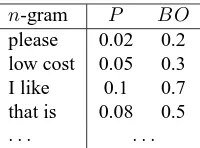
is then computed according to that algorithm above, given the model data organized again in table form as a collection of probabilities and backoff weights for the n-grams appearing in the training corpus. This model displays similarly to that in Table 2.
[image:4.612.136.236.438.512.2]n-gram P BO please 0.02 0.2 low cost 0.05 0.3 I like 0.1 0.7 that is 0.08 0.5 . . . .
Table 2: An English word-based backoffn-gram model. The likelihood and the backoff model score for each n-gram.
4 Weighted finite-state transducers
Weighted finite-state transducers (Mohri et al., 2002) (WFSTs) are defined by means of a tuple (Σ,∆, Q, q0, f, P), whereΣ is the alphabet of
in-put symbols, ∆is the alphabet of output symbols,
Qis a finite set of states,q0 ∈ Qis the initial state,
f : Q → Ris a state-based weight distribution to quantify that states may be final states, and finally, the partial functionP : Q×Σ⋆ ×∆⋆ ×Q → R
defines a set of edges between pairs of states in such a way that every edge is labelled with an input string inΣ⋆, with an output string in∆⋆, and is assigned a transition weight.
When weights are probabilities, i.e. the range of functionsf andP is constrained between 0 and 1, and under certain conditions, a weighted finite-state transducer may define probability distributions. Then, it is called a stochastic finite-state transducer.
4.1 WFSTs for SMT models
Here, we show how the SMT models described in Section 3 (that is, the fiveηscores in the PB trans-lation table, the word penalty, and then-gram lan-guage model) are represented by means of WFSTs.
First of all, the word penalty feature in Equation 8 is equivalently reformulated as another PB score, as in Equations 3 to 7:
h6(s,t) = loge|t|= log max
β6 |β6|
Y
k=1
e|˜tk| (11)
where the length of t is split up by summation using the length of each phrase in a segmentationβ6.
Actually, this feature is independent of β6, that is,
any segmentation produces the expected valuee|t|, and therefore the maximization byβ6 is not needed.
However, the main goal is to introduce this feature as another PB score similar to those in Features 1 to 5, and so it is redefined following the same framework. The PB table can be now extended by means of
η6(˜s,˜t) =e|˜t|, just as Table 3 shows.
Source Target η1 η2 η3 η4 η5 η6
barato low cost . . . e e2
me gusta I like . . . e e2
es decir that is . . . e e2
por favor please . . . e e
. . . .
Table 3: A word-penalty-extended PB translation table. The exponent ofeinη6is the number of words in Target.
[image:4.612.314.539.545.619.2]Translation table
Each PB model included in the translation table, i.e. any PB distribution in{η1(˜s,˜t), . . . , η6(˜s,˜t)},
[image:5.612.321.539.67.189.2]can be represented as a particular case of a WFST. Figure 1 shows a PB score encoded as a WFST, using a different looping transition per table row within a WFST of only one state.
Source Target ηm barato low cost x1
me gusta I like x2
. . . .
...
q0
x1
barato/low cost
me gusta/I like x2
Figure 1: Equivalent WFST representation of PB scores. Table rows are embedded within as many looping transitions of a WFST which has no topology at all; η-scores are correspondingly stored as transition weights.
It is straight-forward to see that the application of the Viterbi method (Viterbi, 1967) on these WFSTs provides the corresponding feature value hm(s,t) for all Features 1 to 6 as defined in Equations 3 to 8.
Language model
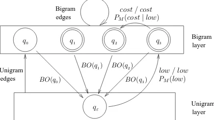
It is well known thatn-gram models are a subclass of stochastic finite-state automata where backoff can also be adequately incorporated (Llorens, 2000). Then, they can be equivalently turned into trans-ducers by means of the concept of identity, that is, transducers which map every input label to itself. Figure 2 shows a WFST for a backoff bigram model. It is also quite straight-forward to see thath7(s,t)
(as defined in Equation 9 for a targetn-gram model where backoff is adopted according to Equation 10) is also computed by means of a parsing algorithm, which is actually a process that is simple to carry out given that these backoffn-gram WFSTs are de-terministic.
q0 q1 q2 q3
BO(q0)
BO(q1) BO(q2)
BO(q3)
qε
Bigram Bigram
Unigram
Unigram layer
layer edges
edges
low / low cost / cost
PM(low)
[image:5.612.72.300.188.358.2]PM(cost|low)
Figure 2: A WFST example for a backoff bigram model. Backoff (BO) is dealt with failure transitions from the bi-gram layer to the unibi-gram layer. Unibi-grams go in the other direction and bigrams link states within the bigram layer.
To sum up, our log-linear combination scenario considers 7 (some stochastic) WFSTs, 1 per feature: 6 of them are PB models related to a translation table while the 7th one is a target-languagen-gram model. Next in Section 4.2, we show how these WFSTs are used in conjunction in a homogeneous frame-work.
4.2 Search
Equation 2 is a general framework for log-linear ap-proaches to SMT. This framework is adopted here in order to combine several features based on WFSTs, which are modelled as their respective Viterbi score.
As already mentioned, the computation of
hm(s,t) for each PB-WFST, let us say Tm (with
1 ≤ m ≤ 6), provides the most likely segmenta-tion βm for s andt according to Tm. However, a constraint is used here so that allTm models define the same segmentationβ:
|β|>0
s = ˜s1. . .˜s|β| t = ˜t1. . .˜t|β|
where the PB scores corresponding to Features 1 to 6 are directly applied on that particular segmentation for each phrase pair(˜sk,˜tk)monotonically aligned. Equations 3 to 7 and 11 can be simplified as follows:
∀m= 1, . . . ,6
hm(s,t) = log max β
|β|
Y
k=1
Then, Equation 2 can be instanced as follows:
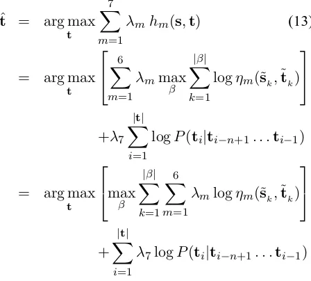
ˆt = arg max t
7
X
m=1
λmhm(s,t) (13)
= arg max t
6
X
m=1
λmmax β
|β|
X
k=1
logηm(˜sk,˜tk)
+λ7
|t|
X
i=1
logP(ti|ti−n+1. . .ti−1)
= arg max t
max
β |β|
X
k=1 6
X
m=1
λmlogηm(˜sk,˜tk)
+ |t|
X
i=1
λ7logP(ti|ti−n+1. . .ti−1)
as logarithm rules are applied to Equations 9 and 12. The square-bracketed expression of Equation 13 is a Viterbi-like score which can be incrementally built through the contribution of all the PB-WFSTs (along with their respectiveλm-weights) over some phrase pair(˜sk,˜tk)that extends a partial hypothesis. As these models share their topology, we implement them jointly including as many scores per transi-tion as needed (Gonz´alez and Casacuberta, 2008). These models can also be merged by means of union once their λm-weights are transferred into them. That allows us to model the whole translation table (see Table 3) by means of just 1 WFST structureT. Therefore, the search framework for single models can also be used for their log-linear combination.
As regards the remaining term from Equation 13, i.e. the targetn-gram language model for Feature 7, it is seen as a rescoring function (Och et al., 2004) which is applied once the PB-WFSTT is explored. The translation model returns the best hypotheses that are later input to then-gram language modelL, where they are reranked, to finally choose the bestˆt. However, these two steps can be processed at once if both the WFST T and the WFST L are merged by means of their compositionT ◦ L(Mohri, 2004). The product of such an operation is another WFST as WFSTs are closed under a composition operation. In practice though, the size ofT ◦Lcan be very large so composition is done on-the-fly (Caseiro, 2003), which actually does not build the WFST forT ◦ L but explores bothT andLas if they were composed,
using the n-gram scores in L on the target hypo-theses fromT as soon as they are partially produced. Equation 13 represents a Viterbi-based compo-sition framework where all the (weighted) models contribute to the overall score to be maximized, provided that the set ofλm-weights is instantiated. Using a development corpus, the set ofλm-weights can be empirically determined by means of running several iterations of this framework, where different values for theλm-weights are tried in each iteration.
5 Experiments
Experiments were carried out on the TED corpus, which is described in depth throughout Section 5.1. Automatic evaluation for SMT is often considered and we use the measures enumerated in Section 5.2. Results are shown and also discussed, in Section 5.3.
5.1 Corpora data
The TED corpus is composed of a collection of English-French sentences from audiovisual content whose main statistics are displayed in Table 4.
Subset English French
T
ra
in SentencesRunning words 747.2K47.5K792.9K
Vocabulary 24.6K 31.7K
D
ev
el
o
p Sentences 571 Running words 9.2K 10.3K Vocabulary 1.9K 2.2K
T
es
[image:6.612.73.297.89.291.2]t Sentences 641 Running words 12.6K 12.8K Vocabulary 2.4K 2.7K
Table 4: Main statistics from the TED corpus and its split.
As shown in Table 4, develop and test partitions are statistically comparable. The former is used to train theλm-weights in the log-linear approach, in the hope that they can also work well for the latter.
5.2 Evaluation measures
with subjective evaluations (the original reason for its success) is actually not so high as first thought (Callison-Burch et al., 2006). Anyway, it is still the most popular SMT measure in the literature.
However, the word error rate (WER) is a very common measure in the area of speech recognition which is also quite usually applied in SMT (Och et al., 1999). Although it is not so widely employed as BLEU, there exists some work that shows a better correlation of WER with human assessments (Paul et al., 2007). Of course, the WER measure has some bad reviews as well (Chen and Goodman, 1996; Wang et al., 2003) and one of the main criticisms that it receives in SMT areas is about the fact that there is only one translation reference to compare with. The MWER measure (Nießen et al., 2000) is an attempt to relax this dependence by means of an average error rate with respect to a set of multiple references of equivalent meaning, provided that they are available.
Another measure also based on the edit distance concept has recently arisen as an evolution of WER towards SMT. It is the translation edit rate (TER), and it has become popular because it takes into ac-count the basic post-process operations that profes-sional translators usually do during their daily work. Statistically, it is considered as a measure highly cor-related with the result of one or more subjective eval-uations (Snover et al., 2006).
The definition of these evaluation measures is as follows:
BLEU: It computes the precision of the unigrams, bigrams, trigrams, and fourgrams that appear in the hypotheses with respect to then-grams of the same order that occur in the translation ref-erence, with a penalty for too short sentences. Unlike the WER measure, BLEU is not an error rate but an accuracy measure.
WER: This measure computes the minimum num-ber of editions (replacements, insertions or deletions) that are needed to turn the system hypothesis into the corresponding reference.
TER: It is computed similarly to WER, using an ad-ditional edit operation. TER allows the move-ment of phrases, besides replacemove-ments, inser-tions, and deletions.
5.3 Results
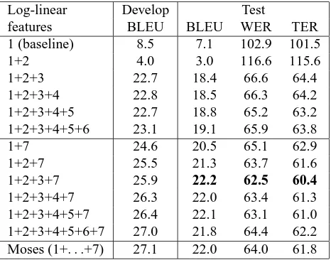
The goal of this section is to assess experimentally the finite-state approach to PB-SMT presented here. First, an English-to-French translation is considered, then a French-to-English direction is later evaluated. On the one hand, our log-linear framework is tuned on the basis of BLEU as the only evaluation measure in order to select the best set ofλm-weights. That is accomplished by means of development data, however, once the λm-weights are estimated, they are extrapolated to test data for the final evaluation. Table 5 shows: a) the BLEU translation results for the development data; and b) the BLEU, WER and TER results for the test data. In both a) and b), the
λm-weights are trained on the development parti-tion. These results are according to different feature combinations in our log-linear approach to PB-SMT. As shown in Table 5, the first experimental sce-nario is not a log-linear framework since only one feature, (a direct PB translation probability model) is considered. The corresponding results are poor and, judging by the remaining results in Table 5, they reflect the need for a log-linear approach.
The following experiments in Table 5 represent a log-linear framework for Features 1 to 6, i.e. the PB translation table encoded as a WFSTT, where different PB models are the focus of attention. Only the log-linear combination of Features 1 and 2
Log-linear Develop Test
features BLEU BLEU WER TER 1 (baseline) 8.5 7.1 102.9 101.5
1+2 4.0 3.0 116.6 115.6
1+2+3 22.7 18.4 66.6 64.4
1+2+3+4 22.8 18.5 66.3 64.2 1+2+3+4+5 22.7 18.8 65.2 63.2 1+2+3+4+5+6 23.1 19.1 65.9 63.8
1+7 24.6 20.5 65.1 62.9
1+2+7 25.5 21.3 63.7 61.6
1+2+3+7 25.9 22.2 62.5 60.4
[image:7.612.314.547.469.652.2]1+2+3+4+7 26.3 22.0 63.4 61.3 1+2+3+4+5+7 26.4 22.1 63.1 61.0 1+2+3+4+5+6+7 27.0 21.8 64.4 62.2 Moses (1+. . .+7) 27.1 22.0 64.0 61.8
is worse than the baseline, which feeds us back on the fact that theλm-weights can be better trained, that is, the log-linear model for Features 1 and 2 can be upgraded until baseline’s results withλ2 = 0.
This battery of experiments on Features 1 to 6 allows us to see the benefits of a log-linear approach. The baseline results are clearly outperformed now, and we can say that the more features are included, the better are the results.
The next block of experiments in Table 5 always include Feature 7, i.e. the target language modelL. Features 1 to 6 are progressively introduced intoT. These results confirm that the target language model is still an important feature to take into account, even though PB models are already providing a sur-rounding context for their translation hypotheses be-cause translation itself is modelled at phrase level. These results are significantly better than the ones where the target language model is not considered. Again, the more translation features are included, the better are the results on the development data. However, an overtraining is presumedly occurring with regard to the optimization of theλm-weights, as results on the test partition do not reach their top the same way the ones for the development data do, i.e. when using all 7 features, but when combining Features 1, 2, 3, and 7, instead. These differences are not statistically significant though.
Finally, our finite-state approach to PB-SMT is validated by comparison, as it allows us to achieve similar results to those yielded by Moses itself.
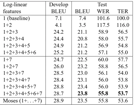
On the other hand, a translation direction where French is translated into English gets now the focus. Their corresponding results are presented in Table 6. A similar behaviour can be observed in Table 6 for the series of French-to-English empirical results.
6 Conclusions and future work
In this paper, a finite-state approach to Moses, which is a PB-SMT state-of-the-art system, is presented. A monotone framework is adopted, where 7 mo-dels in log-linear combination are considered: a di-rect and an inverse PB translation probability model, a direct and an inverse PB lexical weighting model, PB and word penalties, and a target language model. Five out of these models are based on PB scores which are organized under a PB translation table.
Log-linear Develop Test
features BLEU BLEU WER TER 1 (baseline) 7.1 7.4 101.6 100.0
1+2 4.1 3.5 117.5 116.0
1+2+3 24.2 21.1 58.9 56.5
1+2+3+4 24.4 20.8 58.0 55.7 1+2+3+4+5 24.9 21.2 56.9 54.8 1+2+3+4+5+6 25.2 21.2 57.1 55.0
1+7 24.7 22.5 60.0 57.7
1+2+7 26.0 23.2 58.8 56.5
1+2+3+7 28.5 23.0 56.1 54.0 1+2+3+4+7 28.4 23.1 56.0 53.8 1+2+3+4+5+7 28.8 23.4 56.0 53.9 1+2+3+4+5+6+7 28.7 23.8 55.8 53.7
[image:8.612.314.548.63.247.2]Moses (1+. . .+7) 28.9 23.5 55.8 53.6
Table 6: French-to-English results for development and test data according to different log-linear scenarios.
These models can also be implemented by means of WFSTs on the basis of the Viterbi algorithm. The word penalty can also be equivalently redefined as another PB model, similar to the five others, which allows us to constitute a translation modelT composed of six parallel WFSTs that are constrained to share the same monotonic bilingual segmentation. A backoffn-gram model for the target languageL can be represented as an identity WFST whereP(t) is modelled on the basis of the Viterbi algorithm. The whole log-linear approach to Moses is attained by means of the on-the-fly WFST compositionT ◦L. Our finite-state log-linear approach to PB-SMT is validated by comparison, as it has allowed us to achieve similar results to those yielded by Moses. Monotonicity is an evident limitation of this work, as Moses can also feature some limited reordering. However, future work on that line is straight-forward since the framework described in this paper can be easily extended to include a PB reordering modelR, by means of the on-the-fly compositionT ◦ R ◦ L.
Acknowledgments
References
P.F. Brown, S.A. Della Pietra, V.J. Della Pietra, and R.L. Mercer. 1993. The mathematics of machine transla-tion. In Computational Linguistics, volume 19, pages 263–311, June.
C. Callison-Burch, M. Osborne, and P. Koehn. 2006. Re-evaluating the Role of Bleu in Machine Transla-tion Research. In Proceedings of the 11th conference
of the European Chapter of the Association for Com-putational Linguistics, pages 249–256.
D. Caseiro. 2003. Finite-State Methods in Automatic
Speech Recognition. PhD Thesis, Instituto Superior
T´ecnico, Universidade T´ecnica de Lisboa.
S. F. Chen and J. Goodman. 1996. An empirical study of smoothing techniques for language modeling. In
Pro-ceedings of the 34th annual meeting of the Association for Computational Linguistics, pages 310–318.
J. Gonz´alez and F. Casacuberta. 2008. A finite-state framework for log-linear models in machine transla-tion. In Proc. of European Association for Machine
Translation, pages 41–46.
P. Koehn, H. Hoang, A. Birch, C. Callison-Burch, M. Federico, N. Bertoldi, B. Cowan, W. Shen, C. Moran, R. Zens, C. Dyer, O. Bojar, A. Constantin, and E. Herbst. 2007. Moses: open source toolkit for statistical machine translation. In Proc. of Association
for Computational Linguistics, pages 177–180.
S. Kumar, Y. Deng, and W. Byrne. 2006. A weighted finite state transducer translation template model for statistical machine translation. Natural Language
En-gineering, 12(1):35–75.
David Llorens. 2000. Suavizado de aut´omatas y
traduc-tores finitos estoc´asticos. PhD Thesis, Departamento
de Sistemas Inform´aticos y Computaci´on, Universidad Polit´ecnica de Valencia.
D. Marcu and W. Wong. 2002. A phrase-based, joint probability model for statistical machine translation. In Proc. of Empirical methods in natural language
processing, pages 133–139.
Mehryar Mohri, Fernando Pereira, and Michael Ri-ley. 2002. Weighted finite-state transducers in speech recognition. Computer Speech and Language, 16(1):69–88.
Mehryar Mohri. 2004. Weighted finite-state transducer algorithms: An overview. Formal Languages and
Ap-plications, 148:551–564.
S. Nießen, F. J. Och, G. Leusch, and H. Ney. 2000. An evaluation tool for machine translation: Fast evalua-tion for MT research. In Proceedings of the 2nd
in-ternational Conference on Language Resources and Evaluation, pages 39–45.
F.J. Och and H. Ney. 2002. Discriminative training and maximum entropy models for statistical machine
translation. In Proc. of Association for Computational
Linguistics, pages 295–302.
F.J. Och and H. Ney. 2003. A systematic comparison of various statistical alignment models. Computational
Linguistics, 29:19–51, March.
F. J. Och, C. Tillmann, and H. Ney. 1999. Improved alignment models for statistical machine translation. In Proceedings of the joint conference on Empirical
Methods in Natural Language Processing and the 37th annual meeting of the Association for Computational Linguistics, pages 20–28.
F.J. Och, D. Gildea, S. Khudanpur, A. Sarkar, K. Ya-mada, A. Fraser, S. Kumar, L. Shen, D. Smith, K. Eng, V. Jain, Z. Jin, and D. Radev. 2004. A smorgas-bord of features for statistical machine translation. In D. Marcu S. Dumais and S. Roukos, editors,
HLT-NAACL 2004: Main Proceedings, pages 161–168,
Boston, Massachusetts, USA, May 2 - May 7. Asso-ciation for Computational Linguistics.
Kishore Papineni, Salim Roukos, Todd Ward, and Wei-Jing Zhu. 2002. Bleu: a method for automatic evalua-tion of machine translaevalua-tion. In Proceedings of the 40th
annual meeting of the Association for Computational Linguistics, pages 311–318.
M. Paul, A. Finch, and E. Sumita. 2007. Reducing human assessment of machine translation quality to binary classifiers. In Proceedings of the conference
on Theoretical and Methodological Issues in machine translation, pages 154–162.
R. Rosenfeld. 1996. A maximum entropy approach to adaptative statistical language modeling. Computer Speech and Language, 10:187–228.
Matthew Snover, Bonnie Dorr, Richard Schwartz, Lin-nea Micciulla, and John Makhoul. 2006. A study of translation edit rate with targeted human annotation. In Proceedings of the 7th biennial conference of the
Association for Machine Translation in the Americas,
pages 223–231.
J. Tomas and F. Casacuberta. 2001. Monotone statistical translation using word groups. In Proc. of the Machine
Translation Summit, pages 357–361.
A. Viterbi. 1967. Error bounds for convolutional codes and an asymptotically optimum decoding algorithm.
IEEE Transactions on Information Theory, 13(2):260–
269.
Y. Wang, A. Acero, and C. Chelba. 2003. Is word error rate a good indicator for spoken language understand-ing accuracy. In Proceedunderstand-ings of the IEEE workshop
on Automatic Speech Recognition and Understanding,
pages 577–582.
Richard Zens, Franz Josef Och, and Hermann Ney. 2002. Phrase-based statistical machine translation. In Proc.