On the optimal use of put options under trade restrictions

On the optimal use of put options under

trade restrictions

Bell, Peter N

30 October 2014

Online at

https://mpra.ub.uni-muenchen.de/62155/

On the optimal use of put options under trade restrictions

Peter N. Bell

Department of Economics, University of Victoria

Mailing address: BEC 360, 3800 Finnerty Road (Ring Road), Victoria, BC V8P 5C2 Canada.

Abstract

Consider an agent who holds a stock, but is allowed to buy and hold some quantity of

at-the-money put options on the stock. Such an agent must decide the optimal use of financial

derivatives under trade restrictions. This paper uses simulation to compare the optimal quantity

when the agent maximizes mean-variance utility or Value at Risk over wealth at option expiry.

The optimal quantity is larger than the stock holding under mean-variance utility and precisely

the same under value at risk. The options do not remove all variation in returns but still benefit

the agent.

Keywords: Portfolio optimization; put option; trade restrictions; simulation.

JEL Classification: C00, C15, C63, G11, G22.

On the optimal use of put options under trade restrictions

1. Introduction

My objective is to analyze a basic portfolio optimization problem with trade restrictions.

Such a problem is motivated by executive hedging and agricultural insurance, which are two

situations where an agent must hold a risky asset but can trade some kind of financial derivative

on the asset. In general, the agent faces restrictions in terms of their stock holding, the type of

derivatives available, and their ability to trade the derivatives over time; such restrictions are

relevant to a broad set of important portfolio optimization problems.

Corporate executives face trade restrictions on both their stock holdings and their hedging.

Executives often hold large amounts of stock that they cannot trade due to vesting rules or

blackout periods. Executives in the USA are legally able to trade financial derivatives on their

own stock under securities legislation and evidence suggests that it is done (Bettis, Bizjak, &

Kalpathy, 2013). However, executives are subject to a ‘swing profit rule’ that requires them to

forfeit gains from trades on their stock that open and close within a six month period (Schizer,

2000), which means they cannot hedge with dynamic trading strategies.

Farmers also face trade restrictions on their holdings and hedging. Farmers have restrictions

on their holdings because shares in farms do not trade on exchanges like public companies. Crop

insurance provides a hedge for farmer’s production, but the crop insurance contract is restricted

in important ways. For one, farmers can only buy insurance at the start of the growing season

and hold until the end of the season. For another, farmer’s choice over the quantity of coverage

I study the restrictions on executive hedging and crop insurance using simulation. I assume

the agent can only buy at the money (ATM) put options on the stock and must hold the portfolio

constant until option expiry. I suppose that they pick the optimal quantity of options in order to

maximize an objective over wealth at option expiry, either mean-variance utility or the Value at

Risk (VaR) measure. I compare how aggressively the agent hedges under each objective and

find that the agent generally buys such a large quantity of options that the notional value exceeds

the underlying position. However, in each case the option does not remove all variation in

returns.

2. Literature Review

Brown and Toft (2002) suggest that optimal use of financial derivatives deserves more

attention. Perhaps this is because optimal use is generally solved by Mossin’s (1968) result that

it is optimal for a risk-averse agent to buy full insurance when facing risk neutral prices. This

classic result implies the following: if there is an agent who holds a stock and can trade in a

liquid forward market in the stock, then the optimal choice is to sell forwards on the entire stock

position, which eliminates all variation in returns. However, an agent who faces trading

restrictions may not be able to achieve full insurance.

Optimal use of derivatives is generally an issue of complete market models. Carr and Madan

(2001) present a model with a bond, stock, and a continuum of options available at

Black-Scholes prices for all strike prices. Carr and Madan find that investors mainly use ATM strike

prices in equilibrium, which is in line with market experience that ATM options are most liquid.

Liu and Pan (2003) present a model with a stock and two derivatives: one option with strike out

of the money driven by jump risk, and another with strike ATM driven by volatility risk. They

In contrast, optimal use under trade restrictions is an issue of incomplete markets. Duffie and

Richardson (1991) make a pioneering contribution to this literature with a model of an agent who

holds a constant amount of one stock and is only allowed to trade continuously in a futures

contract on another stock with positively correlated returns.

Ahn, Boudoukh, Richardson, and Whitelaw (1999) extend optimal use with incomplete

markets to consider put options. Ahn et al. force the agent to hold a constant amount of stock

and allow them to buy any quantity of put options with any strike. The agent picks the quantity

and strike to minimize VaR for the portfolio, subject to a constraint on the total cost of the hedge.

Deelstra, Vanmaele, and Vyncke (2010) extend the analysis to a general risk measure. Ahn et al.

find the optimal strike is always the same, deep out of the money, while the quantity of options

adjusts to satisfy the constraint. As in my paper, Ahn et al. show that there is more to the

optimal use of options than achieving full insurance.

Ahn et al. (1999) is the most similar to my analysis because the agent holds a constant

position in a stock and buys put options on the same stock. However, there are three differences.

First, Ahn et al. assume the agent has a maximum amount of money to spend on the hedge. I

assume the agent has flexible access to capital, which allows me to identify the optimum in a

broader sense. Second, I assume that the agent uses ATM options. Ahn et al. allow the agent to

buy any quantity of options with any strike price at a cost given by the Black-Scholes model,

which is problematic because tail options are generally illiquid (Carr & Madan, 2001) and more

expensive than Black-Scholes suggests (Liu & Pan, 2003). Third, I use simulation experiments

rather than analytic solutions in order to compare different objective functions.

Research on executive hedging addresses concerns that executives can effectively undo

the Principal-Agent model to explore the effects of executive hedging (Gao, 2009; Boǧaçhan and

Özertürk, 2007). The Principal-Agent model helps study the strategic interaction between an

executive and their company, but it does not identify the optimal use of derivatives in isolation.

This limitation leads me to use the following simulation framework to explore optimal use of

derivatives.

3. Simulation Framework

3.1 Pricing models

I use a standard log-normal probability model for stock prices. I draw a sample of

observations and denote the i-th random draw of the stock price at expiry as Si in Equation (1),

where i is a positive integer. The initial stock price is S0=100 and the returns are normally

distributed Zi with mean µ=0 and standard deviation σ=0.10.

( 1 ) Si = S0e x p (µ+σZi) .

The initial put option price, P, is given by the Black-Scholes model in Equations (2) and (3).

The strike is at the money K=100 and time to expiry is τ=1. For simplicity, the interest rate is

zero throughout, r=0.

( 2 ) d1= ( 1 /σ√τ) ( l o g ( S0/ K ) + ( r + ½σ2)τ) , d2= d1-σ√τ.

( 3 ) P = K e-r τ_{Φ( - d}

2)–S0Φ( - d1) .

The agent’s wealth at expiry is a random variable determined by Equation (4). Wealth is a

function of the random stock price and it depends on the non-random quantity of options as a

parameter, which I denote as W(Si|Qi).

3.2 Objective Functions

I use two objectives defined over the distribution of wealth to identify the optimal quantity.

Both objectives are functions of quantity because they are expectations of wealth conditional on

the quantity of options. I calculate each objective based on a random sample of prices rather

than a population estimates; thus, there is some variation in the estimate of optimal quantity.

The first objective, O1, is the mean-variance utility given in Equation (5). I set the risk

aversion coefficient λ equal to 1.0, which is conventional for simulation experiments and in line

with empirical estimation (Post, van den Assam, Baltussen, & Thaler, 2008).

( 5 ) O1( Qj) = E ( W ( Si| Qj) ) -λV( W ( Si| Qj) ) .

The second objective, O2, is the 5% quantile from the wealth distribution given in Equation

(6). I assume the agent attempts to maximize this objective, which is equivalent to minimizing

VaR because VaR is defined as (S0exp(rt)-w(Qj)) (Ahn et al., 1999).

( 6 ) O2( Qj) = w ( Qj) , w h e r e w ( Qj) : P r ( W ( Si| Qj) < w ( Qj) ) = 0 . 0 5 .

3.3 Solution Method

I use the brute-force search algorithm to estimate the optimal quantity for each objective

function. Brute-force search is a standard algorithm that enumerates the objective function at all

values of the choice variable and identifies the optimum. This algorithm is applicable here

because the optimization is one dimensional (quantity of put options).

The input for the algorithm is a search set for the optimal quantity, Qj∈{Q1,Q2,…QM}, and a

sample of stock prices at expiry,{Si}i=1:N. I use the same search set throughout, which covers an

approximate an exact solution and later use small samples to explore robustness of the optimum.

Given a search set and a random sample, the search algorithm proceeds as follows:

(a) Pick a candidate for optimal quantity, Qj, from the search set.

(b) For each observation on the stock price Si, calculate the wealth W(Si|Qj) as if the agent

bought the quantity Qj. This generates a sample of observations on wealth, {W(Si|Qj)}.

(c) Calculate the objective function based on the sample of observations on wealth.

(d) Repeat steps (a)-(c) for all quantities in the search set. The optimal quantity is that which

gives the largest value for the objective function.

Please note that I provide Matlab code to implement the algorithm and replicate all results in

an appendix.

4. Results and Discussion

4.1 Optimum in large sample

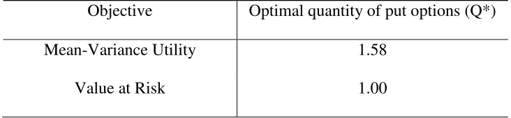
I report the large sample estimate of optimal quantity (Q*) for each objective in Table 1.

Table 1: Optimal quantity of put options for each objective

Objective Optimal quantity of put options (Q*)

Mean-Variance Utility 1.58

Value at Risk 1.00

Table 1 shows that the optimal quantity for the mean-variance utility is larger than one

(Q*≥1). In other words, the notional value for the optimal put option is larger than the

et al. (1999) that the quantity of options must be strictly less than one (p. 363). It also suggests

that the optimal use of financial derivatives may be very different from traditional insurance,

where total coverage must not exceed the value of the asset because of moral hazard (Mossin,

1968).

Table 1 also shows that the optimal quantity for the Value at Risk objective is precisely one

(Q*=1). This gives an example of so-called full insurance, where the amount of coverage equals

the value of the asset and indemnities occur whenever the asset falls below the initial value. This

is a novel result in the literature. In contrast, Ahn et al. find that the optimal strike is always the

same and the optimal quantity adjusts to clear the constraint on the cost of the hedge (1999, p.

368).

4.2 Distribution of wealth with optimal quantity of put options

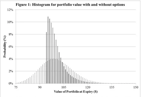
The cost of the optimal hedge for mean-variance utility is small relative to the total portfolio

value ($6.28 for the hedge versus $100 for the portfolio), but the hedge changes the distribution

of wealth at expiry in a significant way. Figure 1 shows the probability distribution for the

Figure 1 shows that the portfolio with the optimal quantity of put options is very different

from the distribution without any options. The probability of either high or low value is smaller

with the portfolio than without. By reducing the frequency and severity of both high and low

values for the portfolio and not changing the average value, the option reduces the variance of

portfolio value and increases the level of mean-variance utility.

4.3 Further analysis of optimal quantity according to Value at Risk

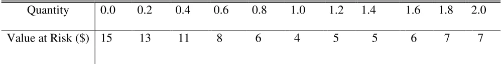
Table 2 shows that VaR is decreasing for small values of quantity and increasing for large

values of quantity. Thus, there is a well-defined minimum for VaR and maximum for the

objective function O2. The columns in Table 2 denote values for quantity of put options and the

Table 2: Value at Risk across different quantities of options

Quantity 0.0 0.2 0.4 0.6 0.8 1.0 1.2 1.4 1.6 1.8 2.0

Value at Risk ($) 15 13 11 8 6 4 5 5 6 7 7

The results in Table 2 challenge the claim in Ahn et al. (1999) that “The VaR is linear in the

hedging expenditure, so each additional dollar generates the same reduction in VaR. There are no

diminishing benefits to hedging” (p. 368). Although I corroborate their result for small

quantities, I find that it is not true for large quantities of options; VaR is actually increasing for

large quantities because the options require large premium payments. The difference in our

results is due to the fact that Ahn et al. use a constrained optimization model, whereas I do not;

Ahn et al. and I consider different subsets of all possible put options. The results in Table 2

suggest that there may be a globally optimal hedge, which would be a new insight for the

literature described here.

4.4 Sampling distribution of optimal quantity

Since the optimal quantity in my model is a sample estimate, it has a sampling distribution. I

report the distribution of optimal quantity in Table 2. I calculate the optimal quantity for 10,000

different samples, each with sample size N=1,000. I use a smaller sample size than Section 4.1

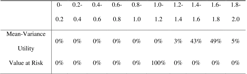
to develop a sense for the robustness of the results to small samples. The columns in Table 3

denote intervals that are closed on the left and open on the right: 0-0.2 denotes the interval [0,

0.2). The entries in Table 3 show the proportion of time that the optimum falls in the interval

Table 3: Sampling distribution of optimal quantity (Q*) for each objective function 0-0.2 0.2-0.4 0.4-0.6 0.6-0.8 0.8-1.0 1.0- 1.2 1.2-1.4 1.4-1.6 1.6-1.8 1.8-2.0 Mean-Variance Utility

0% 0% 0% 0% 0% 0% 3% 43% 49% 5%

Value at Risk 0% 0% 0% 0% 0% 100% 0% 0% 0% 0%

Table 3 shows that the economic interpretation of the optimal quantity for each objective is

robust to resampling under smaller sample size. For mean-variance utility, it is always optimal

to buy options with notional value larger than the underlying position, Q*>1. The difference

between notional and underlying value varies from 20% to 100%, but the interpretation is the

same across all results. For Value at Risk, it is always optimal to take full insurance, Q*=1.

This shows that the knife-edge result first reported for Value at Risk in Table 1 is not restricted

to large samples.

5. Further work

My analysis requires assumptions about the data generating process for asset prices, trade

restrictions, and the agent’s objective function. It is possible to combine different versions of

these assumptions to tackle a broad set of related problems. For example, Bettis et al. (2013)

report that executives typically hedge one third of stock using forwards or collars; it is possible

to replace the put option in my model with a forward or collar and compare the optimal quantity

against the revealed preferences of executives in practice.

For another example, there is some controversy around the appropriate use of mean-variance

1997; Markowitz, 2014). It is possible to consider different objective functions, such as those

described in Post et al. (2008) to further explore the robustness of the optimal choice to model

specification.

Acknowledgements

This research was supported by the Joseph-Armand Bombardier Canada Graduate Scholarship –

Doctoral from the Social Sciences and Humanities Research Council of Canada.

References

Ahn, D.H., Boudoukh, J., Richardson, M., & Whitelaw, R.F. (1999). Optimal risk management using options. The Journal of Finance, 54(1), 359-375.

Barnett, B.J., & Coble, K. (2013). Why do we subsidize crop insurance? American Journal of

Agricultural Economics, 95(2), 498—504.

Basak, S., & Shapiro, A. (2001). Value-at-risk management: optimal policies and asset prices.

Review of Financial Studies, 14, 371–405.

Bettis, J.C., Bizjak, J.M., & Lemmon, M.L. (2001). Managerial ownership, incentive

contracting, and the use of zero-cost collars and equity swaps by corporate insiders. Journal of Financial and Quantitative Analysis, 36(3), 345—370.

Bettis, J.C., Bizjak, J.M., & Kalpathy, S.L. (2013). Why Do Insiders Hedge Their Ownership? An Empirical Examination. Available at SSRN: http://ssrn.com/abstract=1364810

Boǧaçhan, C., & Özertürk, S. (2007). Implications of executive hedge markets for firm value maximization. Journal of Economics & Management Strategy, 16(2), 319—349.

Brown, G.W., & Toft, K.B., (2002). How firms should hedge. The Review of Financial Studies, 15(4), 1283-1324.

Carr, P. & Madan, D. (2001). Optimal positioning in derivative securities. Quantitative Finance, 1, 19-37.

Deelstra, G., Vanmaele, M., & Vyncke, D. (2010). Minimizing the risk of a financial product using a put option, The Journal of Risk and Insurance, 77(4), 767-800.

Duffie, D. & Richardson, H.R. (1991). Mean-variance hedging in continuous time. The Annals

of Applied Probability, 1(1), 1-15.

Gao, H. (2009). Optimal compensation when managers can hedge. Journal of Financial

Economics, 97(2), 218—238.

Jarrow, R.A. & Madan, D.B. (1997). Is mean-variance analysis vacuous: or was beta still born.

Liu, J. & Pan, J. (2003). Dynamic derivative strategies. Journal of Financial Economics, 69, 401-430.

Markowitz, H. (2014). Mean-variance approximations to expected utility. European Journal of Operational Research, 234, 346-355.

Mossin, J. (1968). Aspects of rational insurance purchasing. Journal of Political Economy,

76(4), 553-568.

Post, T., van den Assam, M.J., Baltussen, G., & Thaler, R.H. (2008). Deal or No Deal?

Decision making under risk in a large-payoff game show. American Economic Review, 98(1), 38-71.

Appendix A – Code to replicate results

%% Code Appendix -- Optimal Use of Derivatives % By Peter Bell, October 10 2014

% Written for Matlab to produce all results used in working paper. %

%% Section 1: Global Parameters % Set random number generator

clear all

stream = RandStream('mt19937ar','Seed',12); RandStream.setGlobalStream(stream);

% Calculate option price

S0 = 100; sigma=0.1; K = 100; r = 0;

d1 = (1/sigma)*(log(S0/K)+r+sigma^2/2); d2 = d1 - sigma; O = cdf('norm',-d2,0,1)*K - cdf('norm',-d1,0,1)*S0;

delta = - cdf('norm',-d1,0,1); putPriceDelta=[O delta]; save('Bell-putPriceDelta.txt','putPriceDelta', '-ascii', '-tabs')

% Agent Utility

lambda = 1; %

% Search Set for Optimal Quantity

numQuantSearch = 201; quantScale=100; qStep=1/quantScale;

% numQuantSearch represents # points in search set for quantity % quantScale is parameter to make search set equal to [0,2]

% Parameters for Section 2 -- Large Sample Analysis

sampSizeLarge = 10^6; objectiveTable = zeros(3,numQuantSearch);

% Parameters for Section 3 -- Resampling Analysis

numSimTwo= 10^4; sampSizeSmall = 1000;

% numSimTwo represents # of times that identify optimal quantity (q*) % sampSizeSmall is length of time series, which replaces numPrice

% Goal: Calculate material for Table 1, 2, and Figure 1. %

for numChoice = 1:numQuantSearch qLoop = (numChoice-1)/quantScale; objectiveTable (1,numChoice) = qLoop;

% Simulate large number of prices for each q, calculate objective

S = zeros(1,1); W = zeros(1,1);

S = S0*exp(randn(sampSizeLarge,1)*sigma); W = S + qLoop*(max(K-S,0)-O);

% Mean-Variance Utility

objectiveTable (2,numChoice) = mean(W) - lambda/2*var(W);

% 5% Quantile for distribution

temp2 = sort(W);

objectiveTable (3,numChoice) = -(100-temp2(length(temp2)*5/100)); end

% Table 1: Optimal Choice by Utility

[uMaxMeanVar iMaxMeanVar] = max(objectiveTable (2,:)); [uMaxQuantile iMaxQuantile] = max(objectiveTable (3,:));

qStarMeanVar = (iMaxMeanVar-1)*qStep; qStarQuantile = (iMaxQuantile-1)*qStep;

optimalQuantLarge = [qStarMeanVar qStarQuantile ]

save('Bell-Table1-OptimalQuantityLargeSample.txt','optimalQuantLarge', ... '-ascii', '-tabs');

% Figure 1: Calculate histogram for wealth with optimal derivative

WStarMeanVar = S + qStarMeanVar*(max(K-S,0)-O); histIndex = 75:1:150;

[nZeroPut xOutOne] = hist(S, histIndex);

(nOptimalPut./sampSizeLarge)'];

save('Bell-Figure1-HistogramPortfolioValue.txt','figureOne', ... '-ascii', '-tabs');

% Table 2:

qTemp = 1:20:220;

objectiveQuantile = [(qTemp-1)*qStep;objectiveTable(3, qTemp)]; save('Bell-Table2-ShapeVAR.txt','objectiveQuantile', ...

'-ascii', '-tabs');

%% Section 3: Robustness of results to resampling with small samples % Goal: Build Table 3 in paper (histogram of q* for each utility) %

for simCount = 1:numSimTwo simCount

objectiveTableTemp = zeros(3,numQuantSearch); for numChoice = 1:numQuantSearch

qLoop = (numChoice-1)/quantScale;

S = S0*exp(randn(sampSizeSmall,1)*sigma); W = S + qLoop*(max(K-S,0)-O);

% Log Utility

objectiveTableTemp(1,numChoice) = exp(mean(log(W))); % Mean-Variance Utility

objectiveTableTemp(2,numChoice) = mean(W) - lambda*var(W); % 5% Quantile for distribution

temp2 = sort(W);

objectiveTableTemp(3,numChoice) = temp2(length(temp2)*5/100); end

% Optimal Choice by Utility

[uMaxLog iMaxLog] = max(objectiveTableTemp(1,:));

[uMaxMeanVar iMaxMeanVar] = max(objectiveTableTemp(2,:)); [uMaxQuantile iMaxQuantile] = max(objectiveTableTemp(3,:));

qStarLoop(simCount,1) = (iMaxLog-1)*qStep; qStarLoop(simCount,2) = (iMaxMeanVar-1)*qStep; qStarLoop(simCount,3) = (iMaxQuantile-1)*qStep; end

% Calculate histogram for optimal choice q* across resampling

histIndexTwo = 0:0.2:2;

[qStarHistMeanVar xOut] = hist(qStarLoop(:,2), histIndexTwo); [qStarHistQuantile xOut] = hist(qStarLoop(:,3), histIndexTwo);

tableThree = [ (qStarHistMeanVar./numSimTwo); ... (qStarHistQuantile./numSimTwo)];

save('Bell-Table3-ResamplingOptimum.txt','tableThree', ... '-ascii', '-tabs');