The use of depth averaged currents to estimate bed shear stress as applied to a numerical model of the Sizewell Dunwich Bank area

> ; / e INTERNAL DOCUMENT

l l o

USE OF DEPTH-AVERAGED CURRENTS TO ESTIMATE BED SHEAR STRESS

applied to a numerical model of 3 Sizewell-Dunwich Bank Area

"by

R L SOULSBY

I N S T I T U T E O F O C E A I M O G R A P H I C S C I E N C E S

INSTITUTE OF OCEANOGRAPHIC SCIENCES

Wormley, Godalming, Surrey, GU8 SUB.

(042-879-4141)

(Director: Professor H. Charnock)

Bidston Observatory,

Birkenhead,

Merseyside, L43 7RA.

(051-652-2396)

(Assistant Director: Dr. D. E. Cartwright)

Crossway,

Taunton,

Somerset, TA1 2DW.

(0823-86211)

(Assistant Director: M.J. Tucker)

iVlarine Scientific Equipment Service

Research Vessel Base,

No. 1 Dock,

Barry,

South Glamorgan, CF6 6UZ.

(04462-77451)

(Officer-in-Charge: Dr. L.M. Skinner)

THE USE OF DEPTH-AUEEAGED CUREEBT8 TO

ESTIMATE BED SHEAR STRESS

as applied to a numerical model of

the Sizewell-Dunwich Bank Area

by

E L SOniSBY

This document should not be cited in any paper or report except as

'personal communication', and is for the use of the recipient only.

Institute of Qceanographic Sciences Crossway

Taunton

CONTENTS

Page

8EBCIFICATI0N OF THE PROBLEM: 1

A

PHASE DIFFERENCE BETWEEN % AND U ^ 6

DIFFERENCE IN DIRECTION BETWEEN AND U 1^

SPATIAL DEVELOPMENT OF THE BOUNDARY LAYER 20

IMPLICATIONS FOE SEDIMENT TRANSPORT 26

SUMMAEY, DISCUSSION AND CONCLUSIONS 31

THE USE OF DEPTH-AYEMGED CURREMTS TO ESTIMATE BED SHEAR STRESS

as applied to a nim erical model of the Sizewell—Dunwich Bank area

Specification of the Problem

The problem tackled in this report has arisen in connection with the development

by 108 (T) under contract to Department of the Environment of a two-dimensional

vertically integrated num srical model of current and sediment dynamics over the

Siaewell-Dunwich (S—D) Bank area of the southern Worth Sea, The model is now

almost at the stage where depth—averaged current velocities 0 can be accurately

predicted, given tidal elevation boundary conditions at the three open boundaries,

and the next step is to use these velocities to predict bed shear stresses ^

for insertion into sediment transport formulae,. This informal report presents

the results of a two month study of the feasibility of making this step for the

general case of tidal flow over a sea bed with topography, with application to the

particular case of the S-D Bank.

The problem can be considered in two stages:

1. How accurately can a vertically integrated model predict bed shear stresses,

and would a three—dimensional model be appreciably more accurate.

2. Given accurate stresses, how successfully can they be used in sediment

transport formulae; and if the stresses are inaccurate what error in sediment

transport rates can be expected.

This investigation is chiefly concerned withthe first of these questions. The

second is a topic which is of more general concern to the sedimentation side of

lOS (T) as a whole and will only be discussed briefly. The numerical model itself

might be used to explore some aspects of the second question.

I have tackled the first question from a number of standpoints:

(i) survey of the relevant literature on analytical and numerical models.

(ii) survey of the relevant literature on field observations

(iii) analysis of our own velocity profile measurements made in Lyme and Weymouth Bays

(iv) analysis of Barbara Lees* velocity profile measurements made in the S-D Bank

area.

The area modelled is shown in Fig 1 where the coastline on the western boundary

has been artificially straightened for modelling purposes and the 8m depth contour

arbitrarily chosen to delimit the bank. Also shown are selected grid points of the

model, and the positions where velocity profile measurements have been made.

are shown in Table 1. These values will be used throughout the report to assess

the magnitude of certain flow features when applied to the S-D Bank area.

Parameter

Length of bank

Width of bank

Water depth outside bank

Water depth over bank

Tidal range

Tidal frequency

Goriolis parameter

Max depth averaged valocity

Max friction velocity

Max bed shear stress

Drag coefficient

Roughness length

Vertical eddy viscosity

Symbol L

L

%

10 m

5 m

1.5

1.40x10~4rad,s'

1.15x10-4rad.8"1

100 cm. 8-1

—1

5 cm.s" -1

25 dynes.cm—2

.0025

.05 cm

250 cm2.s-1

Comment s

)

) At 8m contour

From Marconi current

meter data

From Bowden et al

(1959), Red Wharf Bay

Table 1: Typical values for the Sizewell—Dunwich Bank area

The full vertically integrated equations of motion are;

A

& u a O ^ \ ' W - f V

V ^ - 0

~ f

3 c

_cU'

'J

f}

(!)

@ ©

(g)

CO

f W ' f | 0

" 0

"2

f W ' f | 0

Z

©

(g)

where V is the depth averaged velocity in the U direction,^ the surface

elevation, g the acceleration due to gravity, p the water density, ^ has been

resolved into and » and the remaining symbols are defined in Table 1.

t A, ( J

The symbol \J will be used to designate the weak east—west component of current

from the point of view of the model only;

current will be designated \J

in the rest of the report the dominant

The advective terms etc are a good

approximation to the integrals dz. etc provided that the velocity

profile takes one of certain plausible "forms. Horizontal diffusion of momentum

has been omitted from the equation for the present purposes, though for completeness

!

I

c y

\

Marconi *

# # ( I

Tf{£,|0O

/ 645

792\*

A/BS3

/

5-8 KM

— H k — 2 0 0 m grid spacing

Contour values in metres.

Fig. 1. Axea, covered by Sizewell—Dunwich Bank numerical model, with coastline on west artificially

straightened. • 106, selected gridpoints. A BS1, Braystoke current meter stations. >JC Marconi current meter array position.

. STUDY

As a first step towards identifying the role of the various terms in the

present context the model was made to produce time series of each of the

terms throughout a tidal cycle at each of the selected representative

gridpoints shown in Fig 1. The model was run with only the terms 1, 5» 6,

7» 11 and 12 included, as these were thought to be dominant, but the remaining

. A . A

terms were calculated from the values of 1/ and ]/ produced. io%

and were calculated uang a quadratic friction law as will be

if

discussed later. Figs 2 - 7 show that the ^ components on top of the

bank (gridpoints 795 and 6i|.5) represent a balance principally between the

friction and slope terms, with acceleration playing a secondary role and

Coriolis being negligible. At the edges of the bank where the bed slopes

steeply (gridpoints 106 and 792) the advective terms become important.

Figs 8 - 1 3 show that the modelled % components, the friction, slope

and acceleration terms, are all small everywhere. The advective terms,

particularly V ^ V ^ 3^ , are generally large, especially at the edges

of the bank (gridpoints 792 and 801), and the Coriolis term is also

important everywhere. The inclusion of the advective and Coriolis terms

in the model will alter the balance of the terms, possibly in such a way as

to alter their relative importance, but it is likely that the friction term

will remain of primary importance so that its accurate modelling is important

not just from the point of view of sediment transport but also for the

prediction of \J and V • Various of the terms can be associated with

the aspects of the relation between bed shear stress and depth averaged

velocity which will be considered in the succeeding sections: the

acceleration terms with the phase, the Coriolis terms with direction, and

the advective terms with spatial development. As none of the terms is

negligible, all the aspects need to be considered.

Bed shear stress is estimated by the S-D Bank numerical model, in common

with the majority of vertically integrated models, using a quadratic

- 3

where the drag coefficient is constant over the modelled area. Use

of this law assumes that the magnitude and direction of % at a point in

space and at an instant in time is determined, only by the magnitude and

direction of V at the same point and at the same instant. Qu^feation

1 above has been subdivided to investigate this into the questions

(i) Does 'Zc exhibit any time lag' or lead relative to U

(ii) Is the direction of ^ different to that of L/

(iii) Does topography introduce differences in the spatial

distributions of %} and L^jUj

Questions (i) and (ii) are linked, as phase and direction are only

separable by making an artificial distinction, and some of the models

and observations described .consider both. The distinction will generally

be classified by the context. The problem is fundamentally that of

the relationship between near-bottom currents and near-surface currents,

as is closely related to the near-bottom currents, and \J will be

dominated by the near-surface currents. In what follows the behaviour

of will sometimes be approximated by th&t of the near-bottom currents,

and the behaviour of 1/ by that of the geostrophic of free-stream velocity

Wx) . the surface current V' 00 , the surface current Vg , or currents well away from the bed.

The quadratic friction law has been most extensively studied for the case

of steady flow over a flat boundary, so this will be summarised before

progressing to more complicated estimations. Steady turbulent flow over

a flat rough boundary produces a turbulent boundary layer which grows

downstream until it occupies the entire water depth. Near the boundary

the velocity profile has the familiar logarithmic form

K

where 16-(T-ifis von Karman's constant and ^ . Outside this the

velocity is greater than predicted by the log law, by an amount which for a smooth boundary is given by Colijs' wake law (Monin and Yaglom, 1971 )•

Assuming this to hold for a rough boundary gives

4- ^ j" (fs- S -It

where G is the boundary layer thickness, and I T a constant experimentally found to be 0.55 (Fig lU). Assuming fully developed flow (which it may not be)) S - iv , and using S-D Bank values indicates that the log profile alone is valid to better than 10^ throughout the lowest 88% of the water depth? The lowest 15% of this contains a constant stress layer (Hartley and Vincent, 1977; Bradley, 1968). If the flow is very deep and time scales large, such as in the atmosphere or the deep ocean, the free stream flow is geostrophic, and the boundary layer no longer has to grow downstream but has a constant thickness 0-3 ^ v e l o c i t y profile near the boundary follows the log law, whilst above this the velocity increases and veers to match the geostrophic flow at the top of the boundary layer, as described in Section 3« In the l-owest portion of the log layer the shear stress is again roughly constant in both magnitude and direction throughout a layer of thickness 0.2 » where is the geostrophic flow speed (V/imbush and Munk, 1970) Conditions in the S-D Bank, and over large areas of the continental shelf, lie between the extremes of the thin developing boundary layer and the full planetary boundary layer.

Scale length.

Thickness of: Expression

Value for

S-D Bank area Comments

Viscous sub-layer Constant stress layer 12 f O.lS k .027 cm 1.5m

for kinematic viscosity

for ' developing' boundary layer

It ri ti i+.ijm for planetary boundary

layer

logarithmic layer — 7.7m see text for expression

planetary boundary layer Ekman layer

o.3U,/f 130m

66m

see section 3

II If n

Stokes layer 59m see section 2

TABLE 2 Scale lengths for the Sizewell-Dunwich Bank area.

Sediment samples taken by Lees (l977) in the area reveal that over the

bank the bed is composed of fine rippled sand which probably has a ripple

height of somewhere between 1cm and 3cm. This is large compared with the

viscous sublayer thickness so that the flow will be hydrodynamically rough

for most of the tidal cycle. To the west of the bank the bed has a veneer

of fine sand of diameter about 180 yliwi which is probably not rippled

so that here the flow regime will be transitional. To the east there is

gravel 0| maximum length 8cm where the flow will again by hydrodynamically

rough.

The water depth is small, but not negligible, in comparison with the

thicknesses of the planetary boundary layer, Ekraan layer and Stokes layer,

A

so that direction and phase differences between and U are likely

to be correspondingly small but not negligible.

PHASE DIFFERENCE BETWEEN 'To AND U

The use of a quadratic friction law relies on an assumption that is in

phase with 0 throughout the tidal cycle, but it is easily seen that this

need not be so. The equation of motion for the U component of velocity

for a sea uniform in the horizontal directions over a flat horizontal bed

omitting Coriolis terms reduces to

^ f - 5

where ^ is the surface elevation and ^ the shear stress. At a height

'Z~S well away from the bed we will assume that the effect of friction

can be neglected, so that

^ U f s ) r - q

at J 3 % , - 6

L

If the friction term at a height Z - b near to the bed^linearised and assumed

to be proportional to and in phase with the near-bed velocity, then

. = - A ( t ) U ( l > )

f %Z. Z=k - 7

where f\ is a dimensional positive function of Z , so that

% St

- 8

Inserting a sinusoidal tidal time dependence CcS (ft an,i

and re-arranging shows that leads a phase

^ = arc tan ^ /vT^ which is passik positive as A is positive.

is in phase with U(l:^ , and \J is approximately in phase with Uf^for A

typical velocity profiles, so ^ must lead \J

In cases where the terms omitted from the equation of motion above are

retained, or where the friction term is nonlinear, it is not always possible

to define a phase difference, as ^ is no longer sinusoidal. In what

followsJ the term 'phase' is sometimes used in connections with these cases

and should be understood to mean the phase of the dominant harmonic of , or

or for a quadratic friction law, of U,^, =

The theoretical treatment of the problem can be developed by expressing

simplest cast Lamb (1975) asstunes that the eddy viscosity IC is constant

throughout the water depth fv and also constant in time. This is a

particular case of the Stokes shear wave problem, and for our present

purposes the solution for U can be integrated from to to

- i^i ^ _ 9

where R , r fp L 4" -gw 4 " L - Swl>j J ^ j) ^Cejtv i ^

an. U

V

- 1 0

Taking the derivative of the solution for v/ with respect to "Z.

evaluated at the bed

' II I

i: / ( ^ c L I + 0 . ^ )

and ^2. " Crt/ " ^ "1" j

A

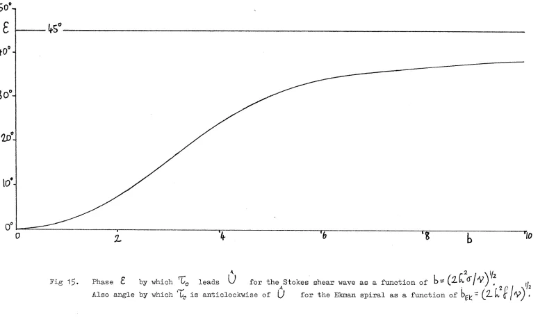
Thus leads U by a phase angle The functional dependence of £

on I) is shown in Fig l5- In the limit as the shear stress is in

phase with the depth-averaged velocity. As the water depth increases the

shear stress exhibits a phase lead over the depth-averaged velocity, tending

towards a lead of 1|.5° as

-For the case of infinitely deep water a suitable scale height 7^^^ is given

by the height at which the fractional departure from the free stream flow —TT

is 6 ,

Fig 1 $. Phase £ by which '0^ leads U for the Stokes shear wave as a function of 1)= ^ , ^|^

to leading w by 1.9° (l° is about 2 mins for the semidiurnal period).

A more realistic form for the eddy viscosity is used by Smith (19773.)

who takes K to increase linearly with distance from the bed but still

to be independent of time. The boundary conditions used are those

corresponding to an infinitely deep sea. Inserting S-D Bank values

A

into his solution indicates that % leads — v by 8°, but it is likely

that if more suitable boundary conditions corresponding to a shallow sea

were used in the solution this value would be much reduced. Bowden et

al (1959) include a Coriolis term in a two layer model in which K is

taken as constant in the upper layer which occupies the top or so of the

flow depth,and the lower friction layer is used solely to provide a boundary

condition at the interface between the layers. Numerical values

corres-ponding to Red Wharf Bay are used which are very comparable to those for

the S-D Bank area, and his results show that ^ (taken as equal to the

stress at the interface) leads U by 1.6 .

A considerable body of work on the numerical solution of shear wave

problems has been produced by Johns, both as applied to sh&llow-water

surface waves (1975, 1977) and to tidal flow in estuaries (1969, 1970,

1976). Throughout the work the friction term is treated using a mixing

length approach, with the mixing length being a specified function of height

above the bed, whose form is chosen to suit the particular problem. The • A

effect of introducing a phase difference between Ic add \J is

discussed by Johns ( 1 9 6 9 ) , but none of the consequences (such as energy

dissipation) discussed lead to a prediction of whether the phase should be rr

positive or negative. A prediction that ic leads [y can be inferred

from velocity profiles presented by Johns (1976), although Ha±^$± neither

"Yg nor iy is actually plotted in this paper. The time-dependence

in which the turbulent kinetic energy equation is introduced into the system

of equations governing the boundary layer dynamics beneath waves so as to

allow transfer and dissipation of turbulence energy. Fig 16 reproduces

this, and it is seen that the time variation of ^ is not simple, nor

is it approximated well by a quadratic friction law. However, it is not

clear how this should be interpreted for the present case of tidal flow

in water of limited depth.

An attractive treatment is given by Vager and Kagan who include

Coriolis terms in the equations of motion and effect closure at the level

of the turbulent energy equation without assuming an artificial functional

dependence for mixing length. Unfortunately the results of the model are

presented for only one particular case, and this with a minimum of discussion.

For a maximum surface velocity of 100 cm s comparable with the S-D Bank,

this case would correspond to a water depth of 70m, which is much deeper

than the S-D Bank^ , It can he roughly estimated from their diagrams that for

this case '(^ leads ly by approximately 20°.

A very similar approach is used by Weatheriy (1975) to model the Florida

Current. The results are discussed in more detail than those of Vager and

Kagan (1969), but are not directly comparable to the S-D Bank case, as

(i) the Florida Current has a residual flow equal in magnitude to the

tidal component, so that the current speed drops to zero but does not

reverse, (ii) the dominant tidal component is diurnal, (iii) the depth is

sufficiently great (800m) that a full planetary boundary layer can develop,

(iv)the flow was stratified, (v) the model was not run for sufficiently

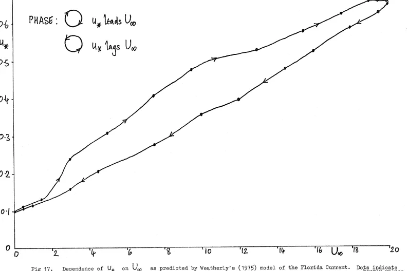
long to allow all transients to disappear. A plot of against time is

given, and this has been rearranged to give the plot of I4,y: against the

free stream velocity, , shown in Fig 17. It can be seen that leads

\y'oo by an amount which can be roughly estimated from the original data

as about 26p. The variation throu^out a tidal cycle of the ratio

.4009

3nv/

Fig 16. The variation of % through one cycle of a wave of period b'ZSs

P H A S f W i s U

C Z ) tfijs u

^2: "4: "6 % 'lo "iz 'f6 U<0

Fig 17. Dependence of U^ on as predicted by Weatherly's (1975) model of the Florida Current. Do|s^indic|te^^

~ ( . Q ) shown in Fig l8 , It is clear that near the start

and end of the cycle, Vgg decreases faster than so that takes

large values. It is of particular interest to note that the thickness

of the boundary layer as determined by the model is very different in both

amplitude and phase to.: that predicted for a quasi-stationary situation.

Turning now from models of tidal flow to field observations we find that

the velocity profiles of Bowden et al (1959) indicate qualitatively that the

near-bed velocity leads the velocity higher up in the flow. Wei sberg and

Sturges (1976) analysed current measurements made in a partially mixed estuary

(Narra gansett Bay) in 12.8m of water, and fognd that velocities at 5.6m

above the bed led those at 10.7m above the bed by about 9° - 13°» They

found good agreement with a simple Stokes shear wave model, though the eddy

2 —1

viscosity they used was only 8cm s which seems rather low, and it is

perhaps more likely that density stratification might account for some of

the observed lead. Harvey and Vincent (1977) found that their measurements

in the southern North Sea in 35® of water were consistent with the near-bed

currents leading those well above the bed, but did not indicate by how much.

Measurements made by Pingree and Griffiths (1974) on the edge of the

continental shelf SW of Lands End in I88m of water indicated a 13° phase

lead of the currents at 3'$™ above the bed relative to those 98m above the

bed for the semi diurnal tidal component. This lead was mainly attributed

to the thermocline descending semidiurnally below 98m, though it seems

plausible that the inertia-friction effects discussed in this section

KBcrks would aiso contribute.

There are also a number of investigators who have found that the near bottom

currents lag behind those nearer the surface. Channon and Hamilton (1971)

analysed measurements made at a number of sites in the western English

Channel and the Bristol Channel in water depths ranging from llpa to lOijm

with maimum tidal current speeds ranging from about 2cm 8"^ g-1 ^

and concluded that there was an appreciable phase lag of bottom current fluctuations bki behind those occurring nearer the surface. Gordon (1975) measured the Reynolds stress and mean velocity 2.25m above the bed in the Choptank estuary in 8m of water with maximum tidal currents of 70 cm s ^, and presented evidence that the stress lagged the mean velocity by a phase which can be estimated from his diagrams as 29°. He attributed this to an increase in the turbulent burst rate during periods of adverse pressure gradient such as occur in decelerating tidal flow, though there is possibly some confusion here between the effects of pressure gradients and those m f spatial accelerations. Indirect evidence is provided by the sediment concentration measurements of Thorn (1975) at various heights in the Thaiaes estuary where the water depth was 19m and maximum tidal velocities were about 110 cm s ^, who found that the sediment concentration lagged behind the mean current velocity. This was attributed to the finite time taken for sediment to diffuse upwards and to settle out, though a lag in the shear stress

relative to the mean velocity could be a contributory factor. This is discussed further by Davies (1977)*

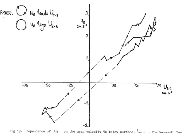
Our own measurements made over a flat uniformly rough bottom in Weymouth Bay, where the water depth was 28m and tidal currents reached 75 cm s ^ have been examined in terms of the phase problem. U,j^ was estimated from near-bed

A velocity profiles averaged over successive 12 min periods, and 1/ is

approximated by ^S-5 , the velocity 5m below the water surface, which was read every 30 mins. is plotted against in Fig 19, and

clearly shows that leads Uc.-c, by a phase which can be roughly estimated as 10°.

I t

'12 J

D

'10 I

Og.

' O h \

" 0 4 .

'0%

0 0

F i g K

%

Variation of % / D through tidal cycle .

as predicted by Weatherly's (197S) model.

' 1

%

3

2jo

HOURS AFTER SLACK WATgR (S-DBAMIC)

&Y ftolDA Cl/kKCWTj

P K A S E i U g _

-IS

%

/

-5o -25^

-1

/

25

u,.

_S-5

"%}

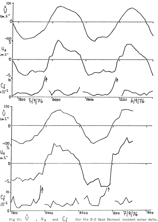
four tidal cycles. To examine the data for phase differences the measurements

were averaged over successive 30min periods ^ Uj£ estimated from the

measurements at 1.2m and 3.2m by assuming that the velocity profile is

log-arithmic up to 3.2m, and L/ estimated by assuming a loglog-arithmic velocity

profile up to 3.2m, a parallelogram rule up to 6.2m, and constant velocity

above that. The assumption of a logarithmic profile up to 3•2m was shown

to be satisfactory by comparing the values with those obtained from

measurements at 1.2m and 2.2m over a period of 1 hr when a meter at 2.2m was

working. Values of U , and are plotted for the four tidal

cycles in Fig 20. is seen to exhibit a 'dwell' after the maximum,

which is similar in form to that found by Johns (l977) and shown here as

Fig 16. The drag coefficient is reasonably steady around a value of

about 2 X 10 ^ over most of each half cycle, but increases rapidly as slack

water is approached. The ratio \J is plotted against phase of

the tide in Fig 18 for the first three half cycles, and is found to agree=

quite well with the curve predi ded by Weatherley's (1975) model, apart

from the time just after slack water.

-Ik

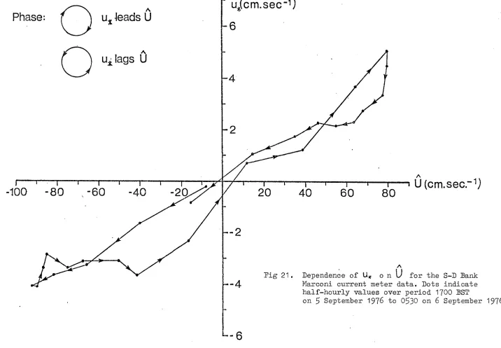
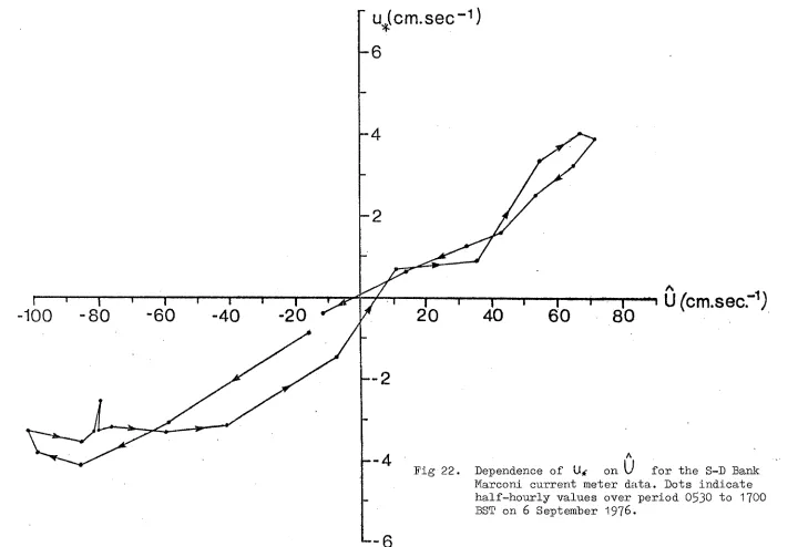
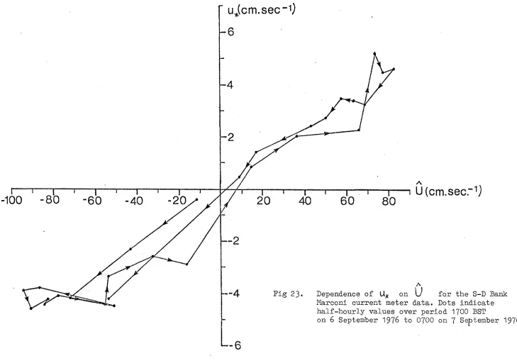
Uif is plotted against L/ in Figs21, from which it can be seen

I'l

that U,jf is not related to ly in a simple way. Considering a

A

clockwise progression on Fig 21 to indicate leading \J and vice

versa, there is a consistent pattern throughout the four tidal cycles of U)g .A

leading \J at times of maximum flow, but lagging LV when

velocities are smaller. The reason for this may be associated with the

Johns-like behaviour referred to above, or may be connected with the presence

of the sand bank.-, It is not appropriate to estimate a value for the phase

difference under the circumstances. The average value of over the

first tidal cycle was found to be .0022 from a linear regression of x b c s c s x

U.

.A, A

, and the average value of

on U U

taken over the same period but excluding a few rogue values was

found to be -2.973, yielding an average value of 2^ = .0^1 cm.

The presence of ripples on the bed is the cause of a similar but distinct

problem. In areas of mobile sand the bed is likely to be rippled which

will increase the total bed shear stress, but the ripple pattern, and hence

the drag coefficient, will change throughout the tidal cycle. Recent work

by Keith Dyer suggests that this may occur in Start Bay. It is possible

that this could be responsible for the complicated behaviour of at the S-D

site discussed above, though it is not known whether the bed at this site

is rippled. The low value of 2^ suggests it is not. However, on

the bank itself, it is expected that the bed is rippled.

A

DIFFERENCE IN DIRECTION BETWEEN % AND U

Some of the models and observations considered in the last section take

account of the effects of the earth's rotation, one consequence of which is

that and C/ need not be in the same direction. The subject has

been considered in some detail since the classical work of Ekman (l90^)

although more attention has been devoted to the case of a wind-induced surface

current than to the bottom boundary layer, and to the steady rather than to

the time-dependent case. In the time-dependent case the veering will, in

general, also be time-dependent.

It is useful to recognise an analogy between the problem of the steady

bottom boundary layer with Ekman veering, and the oscillatory boundary

layer discussed in the previous section. In both cases a horizontally

homogeneous ocean of infinite extent but finite depth C is assumed.

For the case of the oscillatory boundary layer with a periodic forcing

function (Stokes case) the equation of motion neglecting the Coriolis

term is

^ K ( z , t )

-f X.t

"^t fel y - "'2

l%>o oooo

1200 Lia

Fig 20

'0600 '1200

Phase:

-leads U

u j [ c m . s e c - i )

6

lags U

-1C)0 -8C) ', -EH] ' -;2Q

1 U (cm.sec."

- 2

- 4

Fig 21. Dependence of U* o n U for the S-D Bank Marconi current meter data. Dots indicate half-hourly values over period 1700 BST

on $ September 1976 to 0$30 on 6 September 1976.

uicm.sec""'')

Fig 22.

i " I "I U ( c m . s e c . ~ i )

ujcm.sec-1)

- 6

-100

Fig 23.

U ( c m . s e c r i )

Dependence of on U for the S-D Bank Marconi current meter data. Dots indicate half-hourly values over period I7OO EST

uJcm.sec""')

I 1 —

100

- 8 0

20

I

I

40

I

I

60

1

1

80

1

1 U(cm.sec"'')

- 2

./l Fig 2b.

A

Dependence of on U for the S-D Bank

Marconi current meter data. Dots indicate

half-hourly values over period O63O to 1$30 BST on 7 September 1976.

13

with boundary conditions \J^^~0 at Z= 0 and ^L%-(?at

surface 2L~[v • The phase of ih given by "ixlvi

the water

The equations of motion of a bottom boundary layer driven by a steady force

X g including Coriolis terms (Ekman case) are

- I V g = ^ ( ^ K ( r > t ) | y ^ 4 - X .

iU

f a

where is the Coriolis parameter, the earth's angular frequency

and W the latitude. V/riting ? , multiplying the second equation

C t;

by I and adding it to the first equation gives

1

t / 16

Here the boundary conditions are ^ = Q at Z = 0 and Z - L . In

the Ekman case the azimuth of is given by — - I

Equations 13 and l6 are identical in form, and moreover the values of <S and

^ are fairly similar fof a semidiurnal tide in temperate northern

latitudes, so that the phase difference between ^ and W will be similar

in magnitude to the difference between their azimuths. Thus if one of these

problems is important in a particular situation it is likely that the other

will be also. In the preceding section it ^was argued from a consideration

A

of the equation of motion that ^ leads U in phase, which corresponds

A

in the Ekman case to the azimuth of % being less than that of U ,

and the direction of currents generally rotating clockwise with increasing

height above thabed. This will be considered as the positive sense of

veering in what follows. With this analogy between the Ekman veering

problem and the* Stokes shear wave problem the difference in azimuth between

and \J can be obtained from Fig 1^, where the parameter |) becomes

I) —/•=aL3: I for the Ekman case. The azimuth of 0 is h5° clockwise from tk V K /

that of ^ for infinitely deep water, reducing to 0 for water of zero

depth. takes the value 0.9U using S-D Bank numerical values,

for which Fig indicates the azimuth of \J to be 1.7° clockwise from that

of ^ A scale height can be defined as the height above the bed at

-TT which the fractional departure from the free stream flow is £. ,

17

A form for the steady boundary layer was derived without recourse to

artificial assumptions about an eddy viscosity distribution by Csanady

(1967) who postulated that near the bed a logarithmic velocity profile should

exist, while well away from the bed (in an infinitely deep flow) the profile

should obey a velocity defect law. Matching these profiles in an overlap

region yields an expression for the angle iD between ^ and the

geostrophic flow velocity,

The value of has to be determined experimentally. Using A = 5 (Tennekes,

1973) and S-D Bank values indicates that if the water depth were sufficiently

deep, and the flow steady, the total veering would be 38°. However, the

thickness of the boundary layer is shown by the same arguments to be ^

which taking C = O. 3 (Tennekes, 1973) and S-D Bank values gives a boundary

layer thiskness of 130m. In addition there should be no veering within

the logarithmic layer, so we would expect the total veering over the S-D

Bank to be verv much less than in the idealised case.

An extension of Ekroan's work to the case of an oscillatory stress was made

by Faller and Kaylor with boundary conditions appropriate to a

wind-induced surface current on an infinitely deep ocean with eddy viscosity

constant in space and time. A more sophisticated treatment was given by

Smith and Long (1976) who catered for driving forces of wind stress and/or

pressure gradient with any prescribed time dependence, and used an eddy

viscosity which increased linearly from the bed up to a chosen height and

was constant above this.

With neither treatment is it straightforward to obtain an estimate of

the veering for a particular set of conditions, especially as the veering

is now time-dependent, so estimates for the S- D Bank have not been made,

The two-layer model of Bowden et al (19^9) discussed in the previous section

was applied to numerical values appropriate to Red Wharf Bay, and although

veering was not discussed it can be estimated from the results quoted.

At the time when the surface velocity is a maximum the veering between

surface and bottom amounts to 3.1°, whilst when the surface velocity is

a minimum the veering is 60°. Shortly after slack water the veering

becomes slightly negative for a while.

The numerical model of Vager and Kagan (1969) discussed in the previous

section would be ideal for investigating the nature of veering under tidal

conditions, but unfortunately the authors give only a rather inadequate

discussion of results obtained from the model. The account given by

Weatherley (1975) of a very similar model applied to the Florida Current

gives a more thorough discussion of results, although, as discussed in the

previous section, these are not directly comparable to the S-D Bank

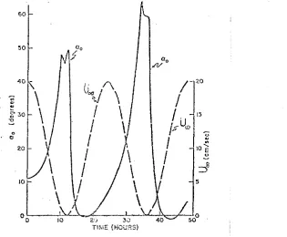
conditions. The time dependence of the total veering calculated by the

model is shown in Fig 25. It is interesting to note that the veering

becomes slightly negative shortly after slack water, as was found by

Bowden et al (1959)- A particularly important finding of this study

was that although the logarithmic layer can be considered as quasi-steady

the total Ekman layer was clearly not quasi-steady.

Field measurements of veering suffer from the limitation that most current

meters give a much less precise reading of direction thpn of speed.

Nevertheless a number of workers have performed experiments which can be

interpreted in this way. Weatherly (1972) made measurements in the Straits

of Florida for comparison with his model, and unexpectedly found that there

was 10.9° of veering between heights of 1m and 3m inside the logarithmic

layer but effectively no turning above this, whereas his model predicted

no veering inside the logarithmic layer but appreciable veering above it.

Harvey and Vincent (1977) working in the southern Horth Sea found about 8°

of veering between heights of 0.58m and 2.96m and about 6,5° of veering

between 2.96m and 10m, indicating that veering was appreciable both within

and above the logarithmic layer. The measurements of Pingree and Griffiths

(1974) on the edge of the continental shelf SW of Lands End show some

scatter in the current directions, but the general indication is a veering

of about 5° - 8° between heights of 2m and 98m.

Veering can be estimated from our own measurements of current speed and

direction at heights of 0.5, 2, l+j 8 and l6m above the bed and 5m below

the water surface at a site in Lyme Bay, 9km from the nearest coastline,

where the water depth varied tidally from 29.5m to 37.5m and the bed was

flat, horizontal and uniformly kigk rough. The maximum current speed 5%

below the surface was 10i| cm s ^. Readings of direction were taken at

each height every 30min over a period of 10.5 hours (with some gaps) and

were the average of three spot readings, each with an accuracy of

± S ° ' The direction reading at 5m below surface may possibly have been

affected by the magnetic influence of the ship's hull. The veering at

each height was calculated relative to the direction at 0.5m. As there

TIME (HOURS)

Pig 2^. The time-dependence of the total Ekman veering (the angle

between the directions of Uco and %e ) for Weatherly's (1975)

numerical model of the Florida Current. For reference the time-dependence of LL is shown.

777,

:: C W)

777777% / / / / /

(c)

(4

Fig 26. Laminar secondary flow around the circular three-dimensional

hump modelled by Smith et al (1977) (a) upstream of the hump, (b) on its forward

behind the hump, technique.

;ace. (c) on the hump's leeward side, (d)

was considerable scatter a meaningful measure could only be obtained by

calculating the mean veering at each height over the 10.5 hr period.

These, together with the standard errors are presented in Table 3.

Height (m) 0 . ^ 2 h 8 16 Surfa CB - 5

S . 0 . — 1.6° 1 . 8 ° 3 . 6 ° 1.8° 7 . 5 °

Mean veering 0° - 0 . 7 ° 0 . 7 ° 0 . 9 ° 2.1:° 31°

Table 3» Veering relative to direction at 0.$m for Lyme Bay data.

The interpretation of a mean veering over a period of the order of a

tidal cycle is doubtful in vidw of the strong time-dependence shown in Fig, 2 2

but is the procedure adopted in all the field observations cited above.

Although the standard errors are large there is an indication that veering

in the correct sense occurs above about 8m, but is effectively zero below

that level. The thickness of the constant stress layer at this site

calculated as Ovu ^ is UO®? so there is no turning within this

layer, as would be expected, nor within the next !#, but appreciable turning

above this.

Finally the Marconi current meter data obtained to the west of the S-D Bank

(Fig 1) which was discussed in the previous section was checked for veering.

One hour at peak flood and one hour at peak ebb during the first tidal

cycle recorded were chosen, and the mean veering relative to the direction

at a height of 1.2m calculated. These angles, together with their

standard errors, are shown in Table U.

Height (m) 1.2 _{3 . 2} L.2 6 . 2

s.e.(flood) - 1.9" 0.6" 0.5"

Mean veering(flood) 0° 1 . 0 ° 2 . 1 ° 3 . 3 °

s.e.(ebb) - 1.h° 1.1° 1 . 3 °

Mean veering (ebb) 0° 2 . 3 ° 3.1° -2.4°

Table it. Veering relative to direction at 1.2m for S-D Bank Marconi data.

Apart from the ebb value at 6.2m the veering is small, but in the

correct sense.

Throughout this section it has been assumed that the sea and sea bed

are horizontally homogeneous and of infinite horizontal extent. In

practice the proximity of a coastline will confine the currents to run

parallel to it, but it is not clear how far from the coast this effect

will be felt.

In addition to Ekman veering the seabed topography may cause secondary

flows which will cause the direction of ^ to be different to the

jA,

direction of . This may be the cause of the negative veering

observed in the S-D Bank area for the ebb tide. The main features of

the secondary flow pattern in a two-dimensional laminar boundary layer

encountering a three-dimensional lump are shown in Fig 2fe, which was deduced

from the theoretical flow field derived by Smith auii et al (1977), though

it is not clear to what extent this carries over to the case of a turbulent

boundary layer. Secondary flow of this sort may well be of greater

significance than Ekman veering in certain cases, but it will not be

considered further because it is likely to be highly dependent on the

particular topography and flow conditions, and hence hard to predict,

SPATIAL DEVELOPMENT OP THE EOUMSAHY LAYER

It has been necessary to assume in most of the previous sections that

the seabed is flat and uniform. If in fact the seabed is not flat, as in

A ^

the case of the S-D Bank, both U and 'Co must vary over the area and

the relationship between them may also vary. We now examine this

relationship, with an assumption that the flow is steady.

I am not aware of any studies of the present problem as such, so two indirect

approaches have been used here. The first approach involves a review of

existing analytical, numerical and observational studies of flow over hills and wavy surfaces, but the results of these studies must be applied

with caution to the S-D Bank situation, as most of the work assumes firstly a deep flow for application to the atmosphere, and secondly two-dimensional topography for ease of analysis. A shallow flow over three-dimensional topography behaves very differently to deep flow over two-dimensional topography; in the former case flow over the top of a bank will be slower than the surrounding flow, because of the large drag in the shallow water, whereas in the latter case it will be faster, to preserve continuity. When two-dimensional continuity can be applied the fastest depth-averaged flow will occur over the crests of the topography, so that if the position of maximum shear stress can be located relative to the topography its displacement from the maximum U is also known. For an isolated hill the displacement will be expressed as a fraction of the length L of the hill measured between the points on the flanks at which the height is I/IO the crest height. For sinusoidal topography the displacement is usually

A, expressed as a phase shift (generally a lead) of relative to U

but for the present purposes it will also be interpreted as a fraction of L where L is now the wavelength. L is roughly 6 km for the S-D Bank.

An analytical approach to deep flow over a two-dimensionally wavy boundary was made by fenjamin (195*9)» who had to assume particular forms for the velocity profile. Using a turbulent-type velocity profile over a wavy

~ /

boundary he found that 'L-j led W by 30° (.083 L ). He found the same lead for a linear profile, whilst for a laminar-type profile he found a lead of 60° (.17 L ) . He generalises the linear profile case to flow over an isolated hill of a specified shape and differentiation of his results shows that the maximum stress occurs a distance .038 L upstream of the crest. A more recent study of deep turbulent flow over a two-dimensional hill by Jackson and Hunt (1975) used an approach more in accord with turbulence theory, though one of the assumptions he made is grossly

invalid in the S-D Bank case. As an example he quoted results for

a hill of the same shape as that of Benjamin. Measured roughly from his

diagram, the maximum occurred at a distance .016 L upstream of the

crest. The problem of deep laminar flow over a three-dimensional hill was

tackled analytically by Smith at al (l977). Their calculations of the

distribution of longitudinal shear stress (for a differently shaped hill

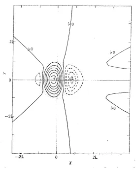
to Benjamin's are shown in Fig 27, from which the maximum shear stress is

seen to lie a distance 0.13 L upstream of the crest. The same topography

may of course give very different results in a turbulent flow. Two

dimensional deep flow over almost sinusoidal sand waves was studied by

Taylor and Dyer (l977) using numerical methods and a plausible turbulence

closure. They found that the maximum stress occurred 19° (•053 L )

upstream of the crest. Using similar techniques over an isolated hill

Taylor (1977a,b) found that the maximum ^ occurred a distance .053 L

upstream of the crest.

Experimental work has also largely concentrated on flows which are

two-dimensional and many times deeper than the height of the topography.

Zilker et al (1977) made measurements over a wavy boundary of steepness

.0125 in fully developed turbulent channel flow and found that the maximum

was located 5 l ° (.14 I- ) upstream of the crest. Similar work was performed

by Smith (1969) over a pair of sinusoidal waves of steepness .O67 in a

flume, with water depths of 7«5 and 6 . 3 times the wave height. In the

first case the first harmonic of the ^ distribution had a phase lead

of (.13!- ) relative to the bedform, whilst in the second case the lead

was 32° ( . 0 8 9 U ). Velocity profiles and bed shear stresses are tabulated

in Smith's report, so that it would be possible, though time-consuming, to

calculate both and U over the waves.

Smith (1969) also made field measurements over a sandwave of height about

3m and length 80m in the Columbia River, USA, with a water depth of 12m

Fig 27. Contours of constant longitudinal shear stress relative to the free-stream value for laminar flow around the circular

three-dimensional hump modelled by Smith et al (1977)' Solid lines

indicate values greater than unity, dotted lines indicate values less than unity, the contour interval is 0.1, and the position of the hump is shaded.

IMTERKiAL B O U N b A U V

LAYER

Rousmness 4 _{K O U S H M E S S 2.}

over the crest. The shape of the sandwave departs sufficiently from

sinusoidal that it is not possible to attribute a phase to ^ r Smith performs

a harmonic analysis of the shape of the wave, and from this synthesises

a predicted shear stress distribution using his own theory which gives

good agreement with the measured shear stress distribution. He also

presents velocity profiles over the wave, which clearly show that the

profile is not locally adjusted over topography of this scale. Field

measurements have also been made by Dyer (l970) over a sandwave. The

measurements of cannot be interpreted in terms of phase as they exhibit

scatter due to the presence of smaller bed features and in addition the mean

stream velocity was varying tidally during the experiment. However it is

again clear that the profiles vary considerably in shape over the wave,

and are not locally adjusted.

The second approach to the problem is to consider adjustment of the

boundary layer over topography by analogy with the adjustment downstream

of an abrupt change of surface roughness. This may give some feel for

the topography problem, although the two problems do have distinct

differences. It is found experimentally that downstream of a roughness

change the surface shear stress adjusts rapidly to its new value (Bradley,

1968) while an internal boundary layer forms, thickening slowly until at a

distance A x downstream the new profile is fully adjusted (Fig 28). Thus

an estimate of shortly after the roughness change should be related

to the profile, and hence v , at a point A . X downstream. The

varying topography can be interpreted as continuously varying surface conditions^

in this case surface displacement, which the boundary layer is continuously

A

adjusting to, so that should everywhere be associated with U at a

distance A x . downstream, with A ) c a function of position. To first order

the error ATj, made in calculating ^ from the local \J will be

= - A x sfc

i£ - 1 5

Since can be roughly calculated from the present model results

for the S-D Bank, an order of magnitude estimate of can be made

provided t\x can be estimated.

A time-scale for development of the logarithmic part of the velocity profile

is given by j where is the height of the log layer. A

disturbance in the log layer will be advected downstream at a velocity close

A A j

to U , SO that a spatial scale for adjustment is given by Z'^ \Jj *

P

If the water depth Iv is sufficiently shallow these arguments can be

extended to the entire boundary layer, giving a crude estimate of as

- 2 0

^65

Fitting S-D Bank values gives A X ^ 2 , 0 0 W ,

A more rigorous argument is given by Miyake in an unpublished thesis

quoted by Busch (l973)t who proposes that the rate of increase of 'Z.\

is proportional to where is now the height of the interface between

the 'old' flow and the internal boundary-layer, so that

IJciz:: c _2i

dx?

where lo is a constant, and U the mean velocity at height Z [ -•

Substituting a logarithmic velocity profile for [J and integrating gives

A )C = ^ ^ ^ C j _ 22

The values of the constants A and Q determined from field and laboratory

experiments over a roughness change are given variously by Busch (1973)

as

/\~ O'h ^ C~ ^

C~D'(>S>

fit is obtained if the value of taken is that for the rougher

surface, and his values of the constants A and 0 will be used here.

The logarithmic velocity profile can be extended to the water surface

without too much error so that 2"^ - . Then as U — U

we have approximately

O ' l f / - 23

This is the distance downstream at which the interface reaches the

surface, and is the distance we will use, though the boundary layer does not

completely reach equilibrium until many times this distance downstream.

Fitting S-D Bank values gives A : t - • This is consistent with

the estimates obtained by the first approach in which the maximum of ^ was

found to be located upstream of the maximum \J by a distance variously

estimated as between .016 L and 0.ll+ [_ , corresponding to 96m to Si+Om

for the S-D Bank.

The numerical model predicts the value of Tc at gridpoint 106 (pig 1)

—2

at the maximum flood velocity to be 28.5 dynes cm , while at a position

_2

200m south the predicted value is 30.3 dynes cm . The flood current is

approximately south going, so that ci To can be calculated from these

figures and inserted in Eq 19, together with the value of found above

to give A^c? = -2.2 dynes cm This represents a 7% error in the

stressywhich should be about the largest error found in the S-D Bank area

as gridpoint 106 has one of the steepest along-tide bed gradients.

Around the S-D Bank there are additionally variations of bed roughness

associated with the various types of bottom sediment. The arguments

given above can equally be applied at a change in bed roughness, and with

greater rigour.

It has been assumed throu^out this section that the flow does not separate

in the lee of the sandbank. Taylor and Dyer (1977) have reviewed the

experimental evidence for separation in the lee of sandwaves, and found that

a most conservative criterion is that the wave sbeepness needs to exceed .0$,

while some workers failed to obtain separation at a steepness of 0.1. As

the steepness at gridpoint 106 is only .01 it is very unlikely that

separation occurs.

IMPLICATIONS FOR SEPIMERT TRANSPORT

The values of To predicted by the S-D Bank model will ultimately be

applied to sediment transport formulae, so it is important to know what

error in sediment transport rate will result from a given error in

Considering bedload transport first, Smith (1969) found that one of the more

reliable formulae was that due to Yalin (1963). When ^0 is much greater

than the threshold bed shear stress this expression for bedload

trans-port rate reduces to

0'6&5 ("p.y) cl

where is the density and c! the diameter of the sediment grains, and

p is the density of water. A fractional error in will cause a larger

fractional error in that a 10% error in would lead

to an error in (j which is greater than 1$^. When ^ is only

slightly greater than the full expression reduces to

/ -7 '/^ 1/1 / \2 / 2/2

- 2S

where ^ is the acceleration due to gravity. In this case a 10% error

in would lead to an error in which is greater than

2S%-A suitable criterion for suspension adapted from the ideas of Bagnold (1966)

is that the ratio \\ir j ( ) where Wg is the settling velocity of the grains

and [(/•^O'Vis von Karman's constant. Using S-D Bank values of U^-5 with

a grain diameter of 180 gives VU^^K/l|^= 1.5 so suspension is

clearly important. The diffusion equation for the mass concentration

of sediment under steady horizontally homogeneous conditions reduces to

k . i!

W 5 C = - K s ^ ' _

where is the eddy diffusion coefficient.

The eddy viscosity coefficient takes the form 1C~ in the lowest

portion of the flow, and provided most of the sediment is confined to this

portion it can be assumed that I C j . " K ' - t h r o u g h o u t the full depth,

as departures from this form higher in the flow will not significantly affect

the sediment. Inserting this in Eq 26 and integrating from a reference

height to the water surface Z - L gives

C H =

f s . ]

^

%

C(Z,~) {z,J - 2 7

The assumption made will generally be valid if \) is sufficiently large, as

will frequently be the case for sand grains in the sea, under which conditions

the form used by Rouse (1937) deriving his well known

k/

concentration profile is unnecessarily complicated. In the lowest part

of the flow the velocity profile is logarithmic, so that if the reference

height is identified with Z q the suspended sediment transport rate is rfv

' J ;

A little work shows that if in addition

1 +

1vi ^ — 29

then the expression in curly brackets is equal to unity to an accuracy

p 0 ^ x

' b (i -try"

O p u w v _ 20

Smith and McLean (1977) find that the reference concentration is well represented by

(•

(4) - Ti fe ~

(h\

%

VP J

_r

provided the excess shear stress is not too large, where is experimentally found to take the value I'Zk'k 10 . Thus

,3 ^ \

31

(Is, =

'

- 32

This expression shows the dependence of on more clearly than does

Einstein's (1950) which cannot be presented analytically as he used the Rouse concentration profile which makes the integration impossible in closed form. The two expressions give almost identical results within the range of

conditions which satisfy the assumptions made here.

On top of the S-D Bank the sand is likely to be rippled, so that 2^ might be expected to take a value of about 0.5cm, and in addition a proportion of the measured value of will be due to the spatially averaged form drag over the ripples. The proportion is often taken as 0.5, so that the maximum value of due to skin friction is 3'$h cm s ^ corresponding to

= 25 dynes cm which taken together with = 3 cm s and

= 2 dynes cm ^, corresponding to I80 yLlM grains, and L = 5% gives b = 2.119 and i f 6 ' % • Thus condition 29 is satisfied and is given by Eq 32 as 0.06l5 gm cm ^s ^ If Tp is increased by 10% and the other values remain the same, Eq 32 gives Cj^ = 0.0859 gm cm ''s \ corresponding to a change of i|.0%.

There are at present still serious shortcomings in the applicability of sediment transport formulae in general. One of these is the problem

referred to above of identifying the contribution to due to form drag

on ripples and larger features, which plays no part in moving the sediment.

This has been examined by Smith and McLean (1977) who showed that the skin

friction velocity over ripples of height H and wavelength A is

related to measured at a height much greater than H by

U

1

^

H

A

1,« q, ( i j

where Q, is a constant and C{) is a drag coefficient for the ripple.

Typical figures for the S-D Bank can be guessed as H = 3cm, A = 20cm,

Z = .O^cm due to grains alone using the value for the area of the

Marconi current measurements assuming it was unrippled; and using

Smith and McLean's experimental values of G, =0.1 and Cp = 0.2 assuming

the flow separates over the ripples gives

r

in comparison with the commonly used figure of 0.5 taken above. Smith (1977)

acknowledges that this is still a contentious area, and it is likely that 2.

r

to this cause.

errors in the estimation of well in excess of_+ 10% can be attributed

He also identifies three other major grey areas in the applicabilityof

C(zi)

sediment transport formulae. Expressions for the reference concentration

have been given by a few workers, but these give widely differing

answers. This subject has not been given the attention it warrants either

theoretically or experimentally and represents a serious source of error.

The non-linear relationship between sediment transport rate and means

that an average value of ^ will give misleading results when used to

estimate sediment transport in naturally occurring situations where is

highly intermittent in both space and time. Lastly there is such a

dearth of field measurements of marine sediment transport that none of the available sediment transport theories can be considered as thoroughly tested.

SOMMARY, DISCUSSION AMD CONCLUSIONS

The relationship between the bed shear stress and the depth

,A

averaged flow velocity U has been examined in terms of differences of

(i) phase of the tidal cycle, (ii) direction, and (iii) spatial distribution,

with particular application to conditions in the Sizewell-Dunwich (S-D) Bank

area.

(i) Analytical and numerical models of oscillatory flow over a flat^bed

(Table 5) show that when the water is sufficiently deep 7^ leads [y by a

phase variously estimated at between 8° and • In shallower depths comparable

to those around the S-D Bank, however, this predicted phase lead reduces to

1.6° to 1.9°J corresponding to 3.2 - 3.8 mins. Field observations in depths

both comparable with and very much deeper than those around the S-D Bank

generally indicate 'Zc leading U by between 9° and 13°, corresponding

to 18-26 mins, although some cases have been reported of Yo lagging U

Analysis of current measurements made in the S-D Bank area shows a complicated

y- i ^ J C" i )

picture with leading [J at times of maximum flow, "but lagging V

when velocities are smaller. The drag coefficient (V' ~ % j [J varies

considerably through a tidal cycle. In areas of mobile sand the changing

ripple pattern will also cause C> to vary and further complicate matters.

(ii) Under conditions of deep steady flow in the northern hemisphere analytical

models of Ekooan veering (Table 6) show that the azimuth of 'lo is less than that

of Q by an angle variously estimated as 38° to » In shallower depths

comparable to those around the S-D Bank this reduces to 1.7°* When the flow

is time-dependent the veering is also time-dependent; for a tidal flow in

shallow water the veering at the time of maximum flow is variously predicted to

be between 3'1° and 6°, though at minimum flow this increases to ^9° to 69°.

The time dependence makes the interpretation of field observations of veering

difficult, because estimates have usually been averaged over a tidal cycle.

Observations made in both deep and shallow water generally indicate mean

veering of 5° - 15°- Analysis of current measurements in the S-D Bank area

at time of maximum flow show veering in the lowest 6.2m of up to 3'3°» An

anomolous value of -2.1|.° in this area may be attributable to secondary flows

associated with the bank. These may be as important a factor in determining

f7" ' '^1

the direction of relative to that of U as Ekman veering, though

more difficult to estimate.

appear to have been systematically studied either analytically, numerically

or experimentally, so that two indirect approaches have been used here.

Analytical and numerical work on deep flow over two-dimensional waves and hills

(Table 7) indicates that the maximum ^ occurs upstream of the maximum

[y by a distance estimated variously as between .016L and .I]!, where L

is the length of the hill or the wavelength of the wave. Laboratory experiments

over a wavy boundary give values between .08% and 0II+L. ,016L-represents

96m in terms of the S-D Bank, and .liiL^represents SUOm. Field observations

in the literature are not easily interpreted in these terms.

The second approach is an analogy with the flow development downstream

of an abrupt change in surface roughness. The interface of the internal

boundary layer which grow downstream of the roughness change reaches the water

surface at a distance 2l|.$m downstream of the change, using S-D Bank numerical

values. This displacement of ^ from i,J can be interpreted as leading to

a 7% error in the estimation of '~Q, at the northern edge of the bank. There

will additionally be similar displacements at the boundaries between zones of

different bed roughness in the area. The flow is unlikely to separate in the

lee of the bank.

The value of ^ obtained from the model represents the sum of the skin

friction acting on the sand grains and the spatially averaged form drag of the

ripples and possibly larger bedforms. The skin friction, needed for insertion

into sediment transport formulae, can only be estimated at present by assuming

an arbitrary partition of the total bed shear stress. The bedload transport

rate is proportional to % ^ ^ at high transport rates, where

is the threshold shear stress, so that a 10^ error in ^ leads to an

error in the transport rate which is greater than 15%. At low transport rates

the error becomes greater than 25%. The maximum shear stress over the S-D

Bank is many times the threshold stress, so that it is likely that suspension

is the dominant mode of transport. A plausible form of equation for the

suspended load indicates that a 10% error in Xo leads to a hOP/o error in the

suspended sediment transport rate in conditions typical of the S-D Bank.

The primary effect of a simple phase lead of relative to \J is

to cause a shift in the time at which sediment moves, but not in the quantity,

so that averaged over a tidal cycle the net transport is unchanged. Thus only

second order effects, such as the introduction of higher harmonics in % ,

the modification of the model's prediction of w , and the need for a

non-stationary sediment transport formula, are felt. As the phase lead is likely

to be only a few degrees in the S-D Bank case, omitting it will probably not

Author Phase by which

leads () Comments

Analytical Models

lamb (1975) 45° Deep water

after Lamb (1975) 1.9° For S-D Bank values

Smith (1977) 8° Deep water

Bowden et al (1959) 1.6° Shallow water Numerical Models

Va^ar & Kagan (1969) 20° Deep water Weatherly (1975) 26° Deep water

Field Observations Weisberg and

Sturges (1976) 9° to 13° Shallow estuary Pingree and

Griffiths (l974j 13° • Deep water Gordon (1975) - 2 9 ° Shallow estuary

lOS(T) 10° Weymouth Bay - fairly shallow

lOS(T) Variable S-D Bank area

Author Angle by which is anticlockwise

of 0

Comments

Analytical Models

Ekman (1905) Steady flow, deep water

Csanady (1967) 38° Steady flow, deep water

after Ekman (1905) 1.7° Steady flow, S-D Bank values

Bowden et al (1959 ) 3.1° Oscillatory flow, max velocity,

shallow water

tt tf ff Oscillatory flow, min velocity,

shallow water

Numerical Model

Weatherly (1975) 6° Oscillatory flow, max velocity,

deep water

II II Oscillatory flow, min velocity,

deep water

Field Observations

Weatherly (1972) 10.9° Deep water

.Pingree and

G r i f f i t h s (l97b)

to 8° _{Deep water}

Harvey and

Vincent (1977)

i4.S° _{Fairly shallow water}

lOS(T) 2 . L ° ( t o 31°?) Lyme Bay - fairly shallow

lOS(T) 3.3°(-2.4°?) S-D Bank area

TA3I.E 6 Veering of 'X^ relative to {J As in Table 5 near-bottom

currents have been identified with and currents away from the bed