Teamwork Efficiency and Company Size

Munich Personal RePEc Archive

Teamwork Efficiency and Company Size

Galashin, Mikhail and Popov, Sergey

New Economic School, Queen’s University Belfast

19 June 2014

Teamwork Efficiency and Company Size

∗

Mikhail Galashin

Sergey V. Popov

June 19, 2014

Abstract

We study how ownership structure and management objectives interact in

deter-mining the company size without assuming information constraints or explicit costs

of management. In symmetric agent economies, the optimal company size balances

the returns to scale of the production function and the returns to collaboration

effi-ciency. For a general class of payoff functions, we characterize the optimal company

size, and we compare the optimal company size across different managerial objectives.

We demonstrate the restrictiveness of common assumptions on effort aggregation (e.g.,

constant elasticity of effort substitution), and we show that common intuition (e.g., that

corporate companies are more efficient and therefore will be larger than equal-share

partnerships) might not hold in general.

JEL: D2, J5, L11, D02.

Keywords: team; partnership; effort complementarities; firm size

∗_{Galashin: New Economic School, Nakhimovsky pr. 47, Moscow, 117418, Russia, mgalashin@nes.ru.}

1

Introduction

Many human activities benefit from collaboration. For instance, writing papers in

Eco-nomics with a coauthor is often much more efficient and fun than writing themsolo. But it is very infrequent that an activity benefits from the universal participation of the whole

human population—a moderate finite group suffices for almost every purpose. So what

determines the size of the productive company? When do the gains from cooperation balance out the costs of overcrowding? Williamson (1971) notes:

The properties of the firm that commend internal organization as a market

substitute would appear to fall into three categories: incentives, controls, and

what may be referred to broadly as “inherent structural advantages.”

We concentrate on the inherent structural advantages of groups of different sizes. We study a model of collaborative production that demonstrates that the answer critically

de-pends on the properties of the production function in a very specific way. Our main

contri-bution is to summarize a generic but hard-to-useeffort aggregationfunction that maps the

agents’ individual efforts to the aggregated effort spent on production with a simpler

team-work efficiencyfunction that measures the comparative efficiency of a team of N workers

against one worker. We demonstrate that many tradeoffs arising from employing differ-ent managerial criteria can be characterized by the interplay of the production function,

which transforms aggregated effort into output, and the teamwork efficiency function. For

instance, to determine what company size maximizes the effort chosen by the company’s

employees, one needs to study the balance between the returns to teamwork efficiency and the behavior of the marginal productivity of the total effort.

We compare the predictions for two types ofcompanies:

team: workers determine their effort independently, and the product is split evenly; and

We attempt to make as few assumptions about the shape of production functions as

pos-sible, which makes us give up the chance to obtain closed-form solutions. However, we are able to obtain comparative static results regarding the change in the optimal size of the

firm due to changes in marginal costs of effort, ownership structure (going from a

worker-owned to capitalist-worker-owned firm and back), and managerial criteria (maximizing individ-ual effort versus maximizing surplus per worker). We demonstrate that the difference in

the sizes chosen by different owners under different managerial criteria are governed by

the direction of change in the elasticity of the production function, and therefore results obtained under the assumption of constant elasticities are misleading. The premise that

elasticities are constant is natural in parametric estimation, but, as we show, assuming

constant elasticities rules out economically significant behavior.

We assume away monitoring, transaction and management costs, direct and indirect,

to guarantee that they do not drive our results. We believe they are an important part

of the reason why firms exist, but they are complementary to the forces we discuss, and their effects have been extensively studied. Our point is that even in the absence of these

costs, there still might be a reason for cooperation—and a reason to limit cooperation.

Ig-noring most issues about incentives and controls allows us to obtain strong predictions, providing an opportunity to test for the comparative importance of incentives in

organiza-tions empirically1_{. Our framework allows one to make judgements about the direction of}

change in the company’s size due to changes in the institutional organization based upon the values of elasticities of certain functions, which can be recovered from the empirical

observations.

We now review the relevant literature. In Section 2, we introduce the model and solve for the effort choice in both the team and the firm. In Section 3, we discuss how to identify

the optimal size of the company. The conclusion follows. The mathematical appendix

contains proofs and elaborates on the characterization of the teamwork efficiency function.

1.1

Literature Review

The paper contributes to two strands of the literature. The moral hazard in teams literature was introduced by Holmstrom (1982), who showed that provision of effort in teams will

be generally suboptimal due to externalities in effort levels and the impossibility of

moni-toring individual efforts perfectly. Legros and Matthews (1993) showed that the problem of deviation from efficient level effort might be effectively mitigated if sharing rules are

well-designed.2 _{Kandel and Lazear (1992) suggest peer pressure to mitigate the 1/N}

ef-fect: the increase of the number of workers lowers the marginal payoff from higher effort.

When the firm gets larger, they argue, the output is divided between a larger quantity

of workers, while they bear the same individual costs. Hence, the effort of each worker

should decrease as firms grow larger, and the peer pressure should compensate for that decrease. Adams (2006) showed that the1/N effect may not occur if the efforts of workers

are complementary enough. Because he uses a CES production function, the determinant

of sufficient complementarity is the value of the elasticity of substitution. Particulary, this means that it’s efficient to either always increase the firm size or to always decrease the

firm size. By generalizing, we in this paper obtain a nontrivial optimal company size.

This allows us to contribute to the firm size literature too. Theories of firm boundaries are classified as technological, organizational and institutional (cf Kumar et al. (1999)). The

technological theories explain the firm size by the productive inputs and ways the

valu-able output is produced. Basically, there are five technological factors that are taken into account in describing the firm size: market size, gains from specialization, management

control constraints, limited workers’ skills, loss of coordination. For example, Adam Smith

explained the firm size by benefits from specialization limited by the market size. By his logic, workers can specialize and invest in a narrower range of skills, hence economizing

on the costs of skills. Becker and Murphy (1992) focus on the tradeoff between

tion and coordination costs. The larger the firm, the larger the costs of management to put

them together to produce the valuable output.

Williamson (1971), Calvo and Wellisz (1978) and Rosen (1982) use loss of control for

explaining the firm size. Williamson points out that the size of a hierarchical organization

may be limited by loss of control, assuming the intentions of managers are not fully trans-mitted downwards from layer to layer. Calvo and Wellisz (1978) show that the effect of the

problem is largely dependent on the structure of monitoring. If the workers do not know

when the monitoring occurs, the loss of control doesn’t hinder the firm size, while it may if the monitoring is scheduled. Rosen (1982) highlights the tradeoff between increasing

returns to scale in management and the loss of control. As highly qualified managers

fos-ter the productivity of their workers, able managers should have larger firms. However, the attention of managers is limited, hence having too many workers results in loss of

con-trol and decreases the productivity of their team substantially. The optimal firm size in

this model is when the value produced by the new worker is less than the losses due to attention diverted from his teammates.

In this literature, Kremer (1993) is the paper closest to ours, because this is one paper

that obtains the optimal size of the firm based solely on the firm’s production function. This paper focuses on the tradeoff between specialization and probability of failure

as-sociated with low skill of workers. He assumes that the the value of output is directly

proportional to the number of tasks needed to produce it. A larger number of workers— and hence tasks tackled—allows for the production of more valuable output, but each

additional worker is a source of risk of spoiling the whole product. Hence, the size of the

firm is explained by the probability of failure by the workers, which correlates with the worker’s skill.

Acemoglu and Jensen (2013) analyze a problem similar to ours. In this paper, agents

pariticipate in anaggregativegame, where the payoff of each agent is a function only of the

agent himself and of the aggregate of the actions of all agents, and they establish existence

for contests. In our game, we allow general interactions, but under certain assumptions

we can summarize these interactions in a similar way, which does not depend on additive separability. Also, Acemoglu and Jensen (2013) and Nti (1997) study comparative statics

for this general class of games with respect to the number of players, whereas we go a

step beyond, looking at the optimal number of players from the perspectives of different managerial objectives. Jensen (2010) establishes the existence of pure strategy Nash

equi-librium in aggregative games but does not explore the symmetry of the equiequi-librium or the

comparative statics.

2

The Model

In this part, we will introduce the model of endogenous effort choice by the company workers as a reaction to the size of the company. We will define the equilibrium, determine

how the amount of effort responds to the change in the company sizeN, and obtain some

comparative statics results.

Company workers contribute effort for production. Efforts{e1, ..., eN}are transformed

intoaggregated effortby theeffort aggregatorfunction:

g(e1, ..., eN|N), (1)

whereg(·|N)changes withN. The aggregated effort is then used for production viaf(·), theproduction function3. Exercising effort lowers the utility of a team member by the effort

costc(e). Obviously, the choice of effort depends upon other members’ effort choice.

3_{This does not have to be a production function. If, for instance,g(·)delivers the amount of effort spent,}

q(g)delivers the quantity produced from employingg efforts, andP(q)is the inverse demand function,

The teammembers split the fruits of their efforts equally. The worker’s problem in the

team is therefore to choose efforteto maximize

u(e|e2, ..., eN, N) =

1

Nf(g(e, e2, ..., eN|N))−c(e). (2)

The firmof sizeN, in line with the literature, acknowledges the strategic

complemen-tarities between workers’ efforts, and provides each worker with a contract that makes this

worker implement the first best effort level. We assume that the residual claimant collects all the surplus; results do not change if the residual claimant only collects a fixed

propor-tion of the surplus, with the rest of the surplus going to the government, to employees

as a fixed transfer, or to pestilence. Workers face the same effort aggregator function and production function.

We introduce a number of assumptions in order to obtain useful characterizations.

Assumption 1. f(·)is strictly increasing and continuously differentiable degree 2.

This is a technical assumption on the production function. We do not require for now

thatf(·)have decreasing returns to scale.

Assumption 2. g(·|N) is symmetric in ei, twice continuously differentiable, strictly

increas-ing in each argument, concave in one’s own effort, and homogenous4 of degree 1 with respect to

{e1, ..., eN}. Normalizeg(1|1)to1.

This assumption states that the identities of workers do not matter, only the amount of effort does. We will be using this assumption extensively, since we will be considering

symmetric equilibria.

4_{Homogeneity of degree of exactly 1 is not a very restrictive assumption: if one hasg(·)which is} homo-thetic of degreeγ, one can useg˜(·) =g(·)1/γ _{andf˜(x) =f(x}γ_{). They produce the same composition, but}

˜

One of the consequences of this assumption is that g′

1(e1, e2, .., eN|N) is homogenous

degree 0. This, in turn, implies that in a symmetric outcome

g′′11(e, e, .., e|N) +g′′11(e, e, .., e|N) +...+g′′1N(e, e, .., e|N) = 0⇔

g₁₁′′(e, e, .., e|N) =−(N −1)g_1i′′(e, e, .., e|N) ∀i∈ {2..N}, (3)

which by concavity in one’s own effort means that in symmetric outcomes, not necessarily everywhere, efforts of members are strategic complements.

Assumption 3. c(·)is increasing, convex, twice differentiable,c(0) =c′_{(0) = 0.}

This immediately implies that every team member exerts a positive amount of effort,

sincef(g(·))is assumed to be strictly increasing at zero.

Example 1. (based on Adams, 2006) Let g(e1, .., eN|N) = PN_i=1eρi

1/ρ

, f(x) = xα_{, c(x) is}

increasing, twice differentiable and concave, andc′_(e)e1−α_{is increasing}5_{. Therefore, agent 1 solves}

max

e1 1

N

N

X

i=1

eρ_i

!α/ρ

−c(e1),

which, assuming a symmetric outcome, producese1 = ...eN =e∗(N) =z(N

α−2ρ

ρ ), wherez(x)is

the inverse ofc′_(x)x1−α_{/α, an increasing function. Hence,e}∗_{(N)is increasing inN if and only if} ρ∈ (0, α/2), and this implies that the effort aggregator needs to be closer to Cobb-Douglas case to

have effort increasing in the team size.

Even for a behaved aggregation function like CES it is hard to obtain a

well-defined argmax_Ne∗_{(N), and this is even harder for other maximands, like the utility of}

a representative agent. This goes against the data: most companies operate with a limited workforce, whatever is the maximand they pursue. In order to understand better what

kind of function can deliver nontrivial predictions (neither 1 nor+∞), we need to

terize the changes ine∗_{(N). The first-order condition of the worker’s problem is}

f′(g(e1, ..., eN)|N))g1′(e1, ..., eN|N)/N−c′(e1) = 0. (4)

Solving the first-order condition is sufficient to solve for the maximum when

f′′(g(e1, ..., eN)|N))(g1′(e1, ..., eN|N))2/N+f′(g(e1, ..., eN)|N))g1′′(e1, ..., eN|N)/N−c′′(e1)<0

(5) for every{e2, ..., eN}. Denoteεq(x) = q′(x)x/q(x), the elasticity ofq(·)with respect to x.

By dividing the second-order condition by the first-order condition and multiplying bye1,

with a slight abuse of notation one can obtain

εf′(g(e₁, ..., e_N|N))ε_g(e₁, ..., e_N|N) +

<0

z }| {

εg′

1(e1, ..., eN|N)−εc′(e1)<0, (6)

which will hold whenever (5) holds.

Assumption 4. (5)holds for every{e1, ..., eN}for everyN.

This holds whenf(·)features decreasing returns to scale, and the aggregator function

g(·)is concave in each argument. Alternatively, one can require thatc(·)is convex enough.

2.1

Effort Choice in a Team: Equilibrium Outcome

The equilibrium is a collection of efforts of agents{e∗

1, ..e∗N}such that each workerisolves

his problem (2) subject to treating efforts of other peers as given:

e∗_i =argmax_e 1

Nf g(e, e ∗ −i|N)

−c(e),

wheree∗

−i denotes values of{e∗1, .., e∗N}omitting the value ofe∗i.

Assumption 5. A unique symmetric equilibrium with nonzero efforts exists.6

Lete∗_{(N)be the function that solves}

f′(g(e∗(N), .., e∗(N)|N))g₁′(e∗(N), .., e∗(N)|N)/N =c′(e∗(N)). (7)

Homogeneity of degree 1 forg(·)helps us to study the behavior ofe∗_{(N). Define}

h(N)≡g(1, ..,1|N).

This function represents the efficiency of coworking. Observe that

h(N) = eg(

Ntimes

z }| {

1,1,1, ..,1|N)

eg(1|1) =

g(

Ntimes

z }| {

e, e, e, .., e|N)

g(e|1) ;

that is,h(N)measures how much more efficient is the team of agents compared to a single

person, holding effort level unchanged. Henceforth we will call itthe teamwork efficiency

function. For instance, if it is linear, the working team is as efficient as its members applying

the same effort separately. By Euler’s rule and symmetry ofg(·),

h(N) = (h(N)e)′_e= (g(e, e, .., e|N))′_e =g′₁(e, .., e)+g₂′(e, .., e)+..+g_N′ (e, .., e) = N g1(e, .., , e|N).

Therefore, (7) can be rewritten as

f′(e∗(N)h(N))h(N)/N2 =c′(e∗(N)). (8)

The equation (8) is the incentive constraint that definese∗_{(N)as a function ofN.}

2.2

Effort Choice in a Firm: First Best

Following Holmstrom (1982), we assume that the residual claimant provides the employ-ees with contracts that implement the first-best choice of effort.

Assumption 6. The first-best choice of effort is positive and symmetric.

The residual claimant would choose the effort sizeeP_{(N)to implement by maximizing}

max

e1,..eN

f(g(e1, e2, .., eN|N))− N

X

i=1

c(ei),

which, assuming a symmetric outcome, leads to the first-order condition

f′_(eP_{(N)h(N))h(N)/N =c}′_(eP_{(N)). (9)}

The solution of (9),eP_{(N), is larger than the solution of (8),e}∗_{(N). The reason is that}

in equilibrium, the marginal payoff to the individual effort does not take into account the

complementarities provided to other workers. Even if the productf(·)were not splitN

ways, but instead were non-rivalrous,7 _{the additional1/N in the marginal benefit of the}

team worker would persist.

2.3

Second-Order Conditions and Uniqueness

Equation (6), the second-order condition of (8), in the symmetric equilibrium can be rewrit-ten as

εf′(e∗(N)h(N)) 1

N +

<0because (3)

z }| {

εg′

1(e

∗_{(N), .., e}∗_(N)|N)−ε

c′(e∗(N))<0. (10)

This is becauseεg(e∗(N), .., e∗(N)|N) = (h(N)/N)e

∗_(N)

e∗_(N)h(N) =

1 N. Let

εf′(e∗(N)h(N))−ε_c′(e∗(N))<0 (11)

hold; then (10) is satisfied automatically. Ifc(x)ismore convexthanf(y)at everyx≥y, this

condition is satisfied. Similar math is used to compare the risk-aversity of individuals: for everyu(x),εu′(x)is just the negative of Arrow-Pratt measure of relative risk aversion.

The second-order condition for (9) is

f′′(eP(N)h(N))h2(N)/N −c′′(eP(N))<0,

which, after dividing by the first-order condition, can be rewritten as

εf′(eP(N)h(N))−ε_c′(eP(N))<0. (12)

Observe that it is very similar to (11): the effort level in the argument is different.

Result 1. Ifεf′(x)is weakly decreasing,ε_f′(x)< ε_c′(x), andh(N)≥1,(11)and(12)are satisfied.

Second-order conditions hold at maxima automatically, but if they hold everywhere, the solution of the corresponding FOC has to be unique. Result 1 thus provides sufficient

conditions for the uniqueness of the pure strategy outcome.

εf′(x)being decreasing has the following interpretation. When ε_f′(x)is constant and

equal to α, it means that f′_{(x) = Kx}α _{+C, which makes f(x) a power function unless}

α =−1, in which casef′(x) = Klnx+C, whereK andC are integration constants. The

decreasingεf′(x)implies “lower power”, or ”less convexity” off(·)at larger arguments.

3

The Optimal Size of the Company

Algebraically, the problem of the optimal firm size with distinct nonatomary agents lies in the discreteness of the firm size. However, using homogeneity and the functionh(N), we

alleviated this mathematical problem. With differentiableh(N), we can take derivatives

with respect toN, and expecte∗_{(N)and e}P_{(N)defined with (8) and (9) to be continuous}

In order to conduct the comparative statics with respect toN, we will apply the usual

implicit function apparatus. For now, h(N) has only been defined for N ∈ {1,2,3, ...}. With a heroic leap of faith, we extend the definition of h(N)to real positive semi-axis.8

We postpone the discussion of how to choose a continuoush(N)if one only wieldsg(·)to

Appendix A.1.

Knowing how the workers of the company of size N choose their effort, we can

char-acterize the consequences of various company managerial objectives on its hiring policy.

Assumption 7. The Problems we study are single-peaked, that is, there is a unique interior

maximum point, and the derivative of every Problem’s Lagrangean is strictly positive below that

point, and strictly negative above that point.

The omitted caveats (multiple local maxima, etc) do not improve the understanding.

3.1

Team Size That Maximizes Effort

In this subsection, we will introduce the apparatus we use to make statements about the optimal size of the company. This subsection is crucial to understanding the further

anal-ysis. We therefore keep the analysis in this part very explicit. Other problems will be dealt

with in a similar fashion, therefore we relocate the repetitive parts to the Appendix. From (8) one can deducee∗_{(N), well-defined over N ∈ R}

+, continuous and

differen-tiable.

Problem 1. CharacterizeN1 =argmaxNe∗(N).

Take elasticities with respect toN on both sides of (8) to get:

εf′(e∗(N)h(N)) [ε_e∗(N) +ε_h(N)] +ε_h(N)−2 =ε_c′(e∗(N))ε_e∗(N).

8_Forg(e

1, e2, ..eN|N) =

q

e2

1+..+e2N +α

P

i6=jeiej,α ∈ [0,+∞)yieldsh(N) =

p

αN2_{+ (1−α)N,}

withεh(N) = 1− 2αN1+(1−α−α), an increasing function ofN whenα < 1and a decreasing function when

εh(N) εf′(e∗(N)h(N))

Φ1 e∗_(N)ր

e∗_(N)ց

N= 1

N= 2

N= 3

N= 4

(a) In(εh, εf′)space

εh(N) εf′(e∗(N)h(N))

Φ1 e∗_(N)ր

e∗_(N)ց

N= 1

N= 2

N= 3

N= 4

(b) Result 2 logic

Figure 1: The choice ofN to maximize effort in a team; and the Result 2 logic

Solve this to obtain

εe∗(N) =

εh(N) (εf′(e∗(N)h(N)) + 1)−2

εc′(e∗(N))−ε_f′(e∗(N)h(N))

. (13)

From (13) one can immediately see that theN that maximizese∗_{(N)has to satisfy}

εh(N) (εf′(e∗(N)h(N)) + 1) = 2. (14)

The denominator of (13) is positive: it is a second-order condition of the effort choice

problem, (11). Therefore, wheneverεh(N) (εf′(e∗(N)h(N)) + 1)>2,e∗(N)is increasing in

N, and otherwise it is decreasing inN.

In the space of(x, y) = (εh(·), εf(·)), Equation (14) simplifiesto:

Φ1 ={(x, y)|x(y+ 1) = 2.}

Solving out the equilibrium will produce a function e∗_{(N), and therefore a sequence of}

values of(εh(N), εf′(e∗(N)h(N)). We depict an example of this path on Figure 1. Denote

For the sequence depicted on the Figure 1, one can observe that e∗_{(N) is increasing at}

N ≤3, and decreasing forN ≥4. Therefore, the optimal “continuous”N (denote itN1) is

between 3 and 4, and the integerN that delivers the maximum effort is either3or4.

The assumption thatg(·) is CES makesεh(N)constant; the assumption that f′(·) is a

power function makesεf′(·)constant. Example 1 predicts that whethere∗(N)is

increas-ing or decreasincreas-ing everywhere depends upon the elasticity of substitution ofg(·)precisely

because, in the world of Example 1,f(x) =xandg(·)is CES.Γ1 is a single point in these

assumptions. Therefore, in order to have a nontrivial prediction about the optimal effort size, one needs either a decreasingεh(N), or a decreasingε′f(·), or both. Obtaining values

in the general case in inherently complicated, but one, however, can make comparative

statics predictions without knowing the precise specification of relevant functions.

Result 2. Whenεf′ is decreasing, an increase (decrease) in the marginal costs of effort leads to an

increase (decrease) inN1. Whenεf′ is increasing, an increase (decrease) in the marginal costs of

effort leads to a decrease (increase) inN1.

Even without knowing the precise values of elasticities, one can obtain useful results.

Assumptions like concavity off can restrict the economically important behavior:

Example 2. (based on Rajan and Zingales, 1998, Lemma 2, p. 398) Letg(e1, ..eN|N) =PN_i=1ei,

and letf(x)be concave. Then

εf′(x) =

f′′_(x)x

f′_(x) <0, h(N) = N ⇒εh(N) = 1,

and therefore, for every N, (εh(N), εf′(e∗(N)h(N))) < (1,1), no matter whatc(·)is. The

indi-vidual effort decreases withN for everyN.

Our results extend to the case when intersections are multiple in a manner similar to

the way that comparative statics with multiple equilibria are treated. We will concentrate

3.2

Firm Size That Maximizes Effort

We will assume that when the firm designs a contract, it tries to implement the first-best, which takes into account the agents’ complementarities in g(·). If a social planner were

choosing the effort for the agents, his FOC would suggest a higher effort for a given N

(see the discussion of the1/N effect on p. 11). Sincec′_{(·)is increasing, this immediately}

implies thateP_{(N)≥ e}∗_{(N), with equality atN = 1, and therefore the effort-maximizing}

sizes of a firm and a team do not have to coincide.

Problem 2. CharacterizeN2 =argmaxNeP(N).

The first-order condition9 _becomes

εh(N) εf′(eP(N)h(N)) + 1

= 1. (15)

Again, if the left-hand side is larger than the right-hand side, the effort is increasing in

N, and the reverse holds when the left-hand side is smaller than 1. The change of the

managerial objective affects multiple components of the optimal size problem:

• The threshold that governs when the firm is big enough,Φ1, is now replaced by

Ψ1 ={(x, y)|x(y+ 1) = 1}.

The reason why2in the definition ofΦ1 is replaced with1in the definition ofΨ1 is

exactly because the marginal1/Neffect, that appeared because individual marginal

benefit did not include the benefits provided to the other participants, went away.

• Since eP(N) > e∗(N) for almost every level of N, the values of ε′_f(eP(N)h(N)) 6=

ε′

f(e∗(N)h(N)), unlessf(·)is a power function in the relevant domain.

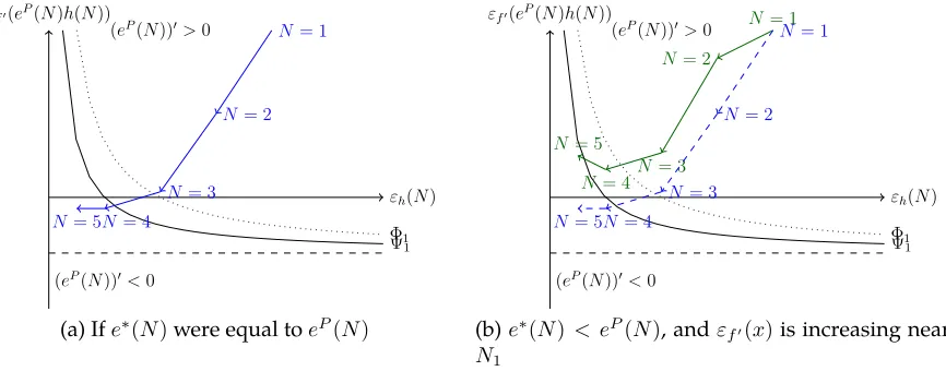
Figure 2a demonstrates the difference, assuming that ε′

f(·) is a decreasing function.

Sinceh(N) did not change, abscissae are the same for different values ofN for both Φ1

εh(N) εf′(eP(N)h(N))

Φ1 Ψ1 (eP_(N))′_>0

(eP_(N))′_<0

N= 1

N= 2

N= 3

N= 4

N= 5

(a) Ife∗_{(N)were equal toe}P_(N)

εh(N) εf′(eP(N)h(N))

Φ1 Ψ1 (eP_(N))′_>0

(eP_(N))′_<0

N= 1

N= 2

N= 3

N= 4

N= 5

N= 1

N= 2

N= 3

N= 4

N= 5

(b)e∗_{(N)< e}P_{(N), andε}

f′(x)is increasing near

N1

Figure 2: ChoosingN to maximize effort, the firm case

and Ψ1. One can see that two effects are at odds: since the threshold is further away,

larger firms become more efficient. However, the change inεf′(·)due to higher efforts for

each firm size might lower the optimal firm size.

Result 3. Ifεf′(x)is weakly increasing, firms that maximize employees’ effort will be larger than

teams that choose their team size to maximize the efforts of the members.

Proof. See Appendix.

3.3

Team Size That Maximizes Utility

Does it make sense to invite more members to join the team? If this increases the utility of other team members, absolutely. Therefore, the team size that maximizes the utility of

a member of the team is the team size that would emerge if teams were free to invite or

expel members.

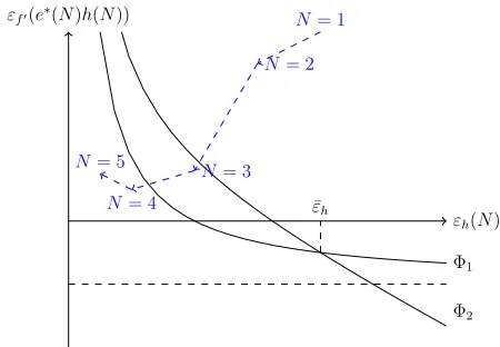
Problem 3. CharacterizeN3 =argmaxN _N1f(h(N)e∗(N))−c(e∗(N)).

N3 should solve the following first-order condition:

εf(e∗(N)h(N))

εh(N) +

N −1

N εe∗(N)

εh(N) εf′(e∗(N)h(N))

Φ1

Φ2 ¯

εh

N= 1

N= 2

N= 3

N= 4

N= 5

Note:Below both graphs both efforts and profits increase as the size of the firm goes larger. Above both graphs both efforts and profits decrease withN. Between graphs, when

εh(N)<εh¯ , efforts increase withN, but profits decrease; the reverse holds whenεh(N)>εh¯ .

Figure 3: ChoosingN to maximize individual utility

Again, at values ofN where the left-hand side is larger (smaller) than 1, the utility is increasing (decreasing) inN. LetΦ2be the set of locations where (16) holds with equality.

This line, evaluated atN =N1, is plotted overΓ1 andΦ1on Figure 3.

One can immediately see that:

• There is a unique intersection ofΦ1 andΦ2, and it happens atε¯h =1/εf(e(N1)h(N1)).

• The path ofΓ1 intersectsΦ1 aboveΦ1TΦ2if and only ifN1 < N3. In general, when

two different maximands are used, different answers are to be expected, but our

result makes issues clearer: the only thing necessary to establish whetherN1 < N3

is the value ofεh(N1)andεf(e∗(N1)h∗(N1)).

Result 4. If εf(x)is increasing (decreasing),εf′(x) + 1 > (<)ε_f(x), and therefore N₃ is larger

(smaller) thanN1.

Therefore, if the elasticity off(·)at the size of the team chosen by team membersN3

is too small, it is likely that the team will be too large to implement high efforts (N3 >

N1). For instance, in teaching, many lecturers assign home assignments for group work.

Some lecturers use fixed group sizes, other lecturers allow students to form groups of their choosing. If higher effort is desirable (for instance, because effort in the classroom

good idea to restrict the group size, against the complaints of students. If the elasticity of

f(·)atN1is larger thanεf′(·) + 1at the sameN₁, students will yearn for increase of the size

of the group, and they will complain that the required group size is too large otherwise.

3.4

Firm Size That Maximizes Utility

This could be a problem for an employee-owned firm, where the residual claimant collects

zero profit and is only necessary to punish deviators for violations of the optimal contract.

Problem 4. CharacterizeN4 =argmaxN _N1f(h(N)eP(N))−c(eP(N)).

AtN4, the following holds (see Appendix for derivation):

εf(eP(N)h(N))εh(N) = 1 (17)

Whenεf(eP(N)h(N))εh(N)>1, the utility of each member of the firm is increasing with

the size of the firm, and the utility is decreasing otherwise.

One can see the difference of (15) and (17): they have to be equal only when∀x, εf(x) =

εf′(x) + 1, which implies thatf(x)is the power function.

Result 5. If εf(x)is increasing (decreasing),εf′(x) + 1 > (<)ε_f(x), and therefore N₄ is larger

(smaller) thanN2.

Proof. See Appendix.

This Result helps to establish why people do not work efficiently in different

environ-ments. The problem is not so much in the returns to scale of the production function, the

relevant threshold is the comparison of the first and second derivativeÑŃ of the produc-tion funcproduc-tionÐś which boils down to whether the elasticity of the producproduc-tion funcproduc-tion is

locally increasing or decreasing. Those employee-owned companies, whose employees

feel that they would be more motivated and would work harder had they had more col-laborators, haveεf(eP(N)h(N))< εf′(eP(N)h(N)) + 1, their production function is locally

Results for other managerial objectives can be obtained in a similar fashion: for

in-stance, a residual claimant that collects a fixed proportion of the total surplus of the firm will employmore than N4 workers as long as (12) holds. We reserve these for the future

research.

3.5

The Quagmire Of Constant Elasticities

The previous analysis showed that at least one of two elasticities cannot be constant in

order to obtain a well-defined optimal company size. However, even holding one of two elasticities constant can mislead. In the following example, we assume thatεh(N)is

de-creasing from a large enough value to0, whereas the production function is a power

func-tion.

Example 3. Letf(x) = xα_{andc(e) = e}β_{. Letβ > α > 0, then relevant Assumptions and(11)}

are satisfied. For general but convenienth(·), whereεh(·)is decreasing, the first-besteP(N)chosen

by the firm satisfies

α(eP(N)h(N))α−1h(N)

N =β(e

P_(N))β−1 _⇒

eP(N) = exp

lnα−lnβ

β−α +

α

β−αlnh(N)−

1

β−αlnN

.

The effort sizee∗_{(N)chosen by the members of the team satisfies}

α(e∗(N)h(N))α−1h(N)

N2 =β(e

∗_(N))β−1 _⇒

e∗(N) = exp

lnα−lnβ

β−α +

α

β−αlnh(N)−

2

β−αlnN

.

Let us order firm sizes chosen with different managerial objectives. Whenεh(N)is decreasing,

1. N1, the team size that maximizes the effort when the effort level is chosen simultaneously and

independently, satisfiesεh(N1) = 2/α;

N εh(N)

εh(N)

2_/α

1_/α 2_/β

1_/β

N1 N2 N3 2(N−1)

N β−α

(a) Whenβ >2α

N εh(N)

εh(N)

2_/α

1_/α 2_/β

1_/β

2(N−1)

N β−α

N1 N3N2

(b) Whenβ <2α

Note:N₂=N₄in both cases becausef(·)is a power function.

Figure 4: Ordering solutions from Example 3

3. N3, the team size that maximizes the team member’s utility when the effort level is chosen

si-multaneously and independently, solvesεh(N) = 2(N_{N β}−₋1)_α, right-hand size of which is

mono-tone, and converges to2/βfrom below.

4. N4, the firm size that maximizes the utility per worker10 when the effort level is chosen

ac-cording to the first best, satisfiesεh(N4) = 1/α;

Example 3 supplies the following intuition for different maximands (see Figure 4):

1 & 2 Effort-maximizing size of the firm is larger than the effort-maximizing size of the team. This is a consequence off(·)being a power function (see Result 3), and does

not have to hold in general.

1 & 3 The company size chosen by the team when the effort level is chosen individually

is smaller than the company size chosen to maximize the effort size. This is not

a general result, but a consequence of a strong connection between εf(·) = α and

εf′(·) = α − 1. Compare (14) and (16): when N is such that (8) is satisfied, (16)

suggests that the utility of each participant would go up if the size of the team went

down.

2 & 4 The size of the firm that maximizes employees’ utilities is maximizing their effort as

well. This is not a general result, but a direct consequence off(x) = xα_{: conditions}

(15) and (17) coincide algebraically.

3 & 4 When a self-organized team becomes incorporated, it might become larger or smaller.

If 2α < β, then the incorporated firm becomes smaller than the team. Otherwise,

the firm can become larger, but only whenN3 >1/(2−β/α).

This exercise demonstrates many spurious findings arising simply from the desire of closed form solutions. Some of the strong predictions are generalizable, but most are a

consequence of the power function assumptions.

4

Conclusion

In this paper, we stepped away from the common assumptions about production functions

to study the effects of scale on the optimal size of a company from many perspectives. Our contribution is to circumvent the inherent discontinuity in hiring when complementarities

are important. We found ways to characterize the effects of changes in the management

of the company, like incorporation of a partnership, or going from private to public, on hiring or firing, and whether employers’s effort will suffer from overcrowding or from

insufficient specialization. We found that teams do not have to be larger or smaller than

firms that use the same production function. The analytic framework we suggest is very general, and can be modified to include uncertainty, non-trivial firm ownership (for

in-stance, one worker can be the claimant to the residual profit, with nontrivial implications

on the effort choice), non-trivial wage schedules (for instance, imperfect observability of effort, total or individual, can call for the design of the optimal wage schedule), or

profit-splitting schemes from cooperative game theory like the Shapley value.

The homogeneity of workers is important in our analysis. We have obtained results for heterogenous workforce, where some workers are capable (can choose a positive effort

be the case that the incapable workers are employed along with capable ones: this happens

if the effort aggregation function is such that the employment of an extra person provides teamwork efficiency externalities for the capable workers, whereas additional effort from

the hired capable person would diminish the productivity of other capable employees.

A

Mathematical Appendix

Solution of Problem 1in text, on page 13.

Solution of Problem 2To choose the firm size that maximizes the level of effort, take the

derivative of both sides of

f′(eP(N)h(N))h(N)/N =c′(eP(N))

with respect toN. The values ofN where(eP_(N))′ _{= 0will be the one we are looking for.}

The derivative looks like

f′′(eP(N)h(N))[h(N)(eP(N))′+h′(N)eP(N)]h(N)/N+f′(eP(N)h(N))[h′(N)/N−h(N)/N2] =

=c′′(eP(N))(eP(N))′.

Divide by the first-order condition to obtain

f′′_(eP_{(N)h(N))[h(N)(e}P_(N))′_+h′_(N)eP_(N)]h(N)/N+f′_(eP_(N)h(N))[h′_{(N)/N −h(N)/N}2_]

f′_(eP_{(N)h(N))h(N)/N} =

= c

′′_(eP_(N))(eP_(N))′ c′_(eP_(N)) .

Rearrange to obtain

c′′_(eP_(N))eP_(N)

c′_(eP_(N)) −

f′′_(eP_{(N)h(N))h(N)e}P_(N)

f′_(eP_(N)h(N))

(eP_(N))′_N eP_(N) =

h′_(N)N h(N)

1 + f

′′_(eP_(N)h(N))

f′_(eP_(N)h(N))

Rewrite:

εeP(N) =

εh(N) εf′(eP(N)h(N)) + 1

−1

εc′(eP(N))−ε_f′(eP(N)h(N))

.

When εh(N) εf′(eP(N)h(N)) + 1

> 1, effort increases with the size of team, and effort

decreases otherwise.

Solution of Problem 3To choose the team size that maximizes utility, solve

max

N

1

Nf(h(N)e

∗_(N))−c(e∗_(N)),

wheree∗_{(N)is such that (8) holds. The first-order condition is:}

f′(e∗(N)h(N)) (e∗(N)h′(N) + (e∗(N))′h(N))/N−f(e∗(N)h(N))/N2−c′(e∗(N))(e∗(N))′ <> 0,

with a>sign when the utility of each team member is increasing in the membership size, with a<when the utility of each member is decreasing in the membership size, and with

equality at optimum. Substitute (8):

f′(e∗(N)h(N)) (e∗(N)h′(N) + (e∗(N))′h(N))/N −f(e∗(N)h(N))/N2−

f′(e∗(N)h(N))h(N)/N2(e∗(N))′ <> 0.

Group variables and divide byf(e∗_(N)h(N))/N2 _{>0to obtain}

f′_(e∗_(N)h(N))(e∗_(N)h(N)) f(e∗_(N)h(N))

e∗_(N)h′_{(N)N + (e}∗_(N))′_{h(N)(N −1)}

(e∗_(N)h(N))

−1<>0,

εf(e∗(N)h(N))

εh(N) +

N −1

N εe∗(N)

−1<>0.

Solution of Problem 4 To maximize the utility of each member of the team when their

effort is imposed to deliver the first best outcome, the size of the firm should be chosen to

solve

max

N f(e

P_(N)h(N))1

N −c(e

subject to (9). The first-order condition of this problem is

f′(f(eP(N)h(N)))[eP(N)h′(N)+h(N)(eP(N))′]1

N−

1

N2f(e

P_(N)h(N))−c′_(eP_(N))(eP_(N))′ _<>0.

Divide byf(eP_(N)h(N))/N2 _{and rearrange to obtain}

1

f(eP_(N)h(N))/N2 εf(e

P_(N)h(N))ε

h(N)−1

<>0. (18)

Result 1. For every level of efforte,

εf′(eh(N))< ε_f′(e)< ε_c′(e).

Using the effort levels implied by either equilibrium outcome or first best completes the

proof.

Lemma 1. Let ˜e(N) > e(N). Ifεf′(·)is weakly decreasing (increasing), the effort-maximizing

team size under˜e(N)is lower (higher) than the effort maximizing team size fore(N).

Lemma 1. LetN1andN˜1be solutions to team effort maximizing problems with effort

func-tionse(N)ande˜(N)respectively. Ifεf′(·)is weakly decreasing, sincee(N)<e˜(N)

εh( ˜N1)

εf′(e( ˜N₁)h( ˜N₁)) + 1

−2≥εh( ˜N1)

εf′(˜e( ˜N₁)h( ˜N₁)) + 1

−2 = 0.

Since we assumed that the problem is single-peaked, this implies that the effort is

increas-ing withN fore(N)atN = ˜N1, or thatN1 >N˜1. The result for increasingεf′(·)is proven

similarly.

Result 2. Suppose the marginal costs decrease toc˜′_(x)≤c′_{(x)for anyx. Consider}

symmet-ric equilibrium effortse(N)for the initial problem andc(·)costs, ande˜(N)under modified

c′_(x)and˜c′_{(x)respectively. Therefore,}

f′(e(N)h(N))h(N)/N2−c˜′(e(N))≥0 = f′(˜e(N)h(N))h(N)/N2−˜c′(˜e(N)).

This, combined with second order conditions and single crossing, implies˜e′_{(N) ≥ e(N).}

Applying Lemma 1, we obtain the result.

Result 3. LetN˜1 solve

εh( ˜N1)

εf′(eP( ˜N₁)h( ˜N₁)) + 1

−2 = 0.

Then _N˜_{1 ≤ N2 by single-peakedness assumption for Problem 1. Moreover, by Lemma 1,} ˜

N1 ≥N1 aseP(N)≥e∗(N)for eachN. Hence,N2 ≥N˜1 ≥N1.

Result 4. Observe that

(εf(x))′ = (εf′(x) + 1−ε_f(x))

εf(x)

x .

Sincef(·)is an increasing function, the first part of the statement is proven. The second part of the statement follows immediately from evaluating (16) atN1.

Result 5. εf(x)≥εf′(x) + 1means

εf(eP(N2)h(N2))εh(N)−1≥(εf′(eP(N₂)h(N₂)) + 1)ε_h(N)−1 = 0

Workers’ utility increases atN2, hence by single-peakedness assumptionN2 ≤N4.

A.1

The Choice of

h

(·)

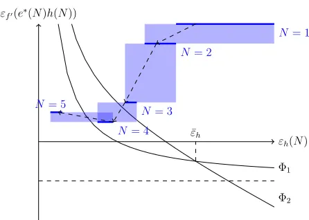
If one knows f(·), h(·), and c(·), one can conduct the analysis above. However, h′_(N)is

not a fundamental, at least not in non-integer values. It suffices to knowh(N)to evaluate

e∗_,eP_,ε

h′_{(N) as well. h}′_{(N)values at integer points would suffice, since optimization requires}

checking whether the value of the elasticity ofh(·)is above or below a certain threshold. How can one choose the value ofh′_{(N)at integer points if one only knowsh(N)at integer}

points? Obviously, arbitrary choices ofh′_{(N)can position the points all over the space of}

(εh, εf′). One can impose a refinement over the possible derivatives ofh(N):

h′(N)∈[min(h(N + 1)−h(N), h(N)−h(N −1)),max(h(N+ 1)−h(N), h(N)−h(N −1))].

(19) To connect integer points, assume that between two neighboring integers,h′_(N)is

mono-tone. This implies that extrema ofh(N) are only at integer points. Obviously, this

pre-serves concavity, convexity and monotonicity, had h(N) defined over integers had these properties. This limitation helps a lot in characterizing the optimal paths. Consider

Fig-ure 5, which is similar to FigFig-ure 3, but instead ofpointsalong the path ofΓ1, we plotsets

for every value ofεf′(e∗(N)h(N))that is consistent with some value ofh′(N)restricted by

(19) at integer values, and then impose monotonicity forh(·)across the path to connect the

integer values. On Figure 5, one can see that the intersection withΦ1 happens between

N = 3andN = 4, whereas forΦ2intersection withΓ1happens betweenN = 4andN = 5.

Therefore, forf(·)andg(·)behind Figure 5, the self-organizing team will be too large to

maximize efforts.

The reverse problem of obtainingg(·)if one knowsh(·)but notg(·)is surprisingly easy.

Result 6. For everyh(N),

g(e1, .., eN|N) =h(N) (e1e2...eN)1/N

and

g(e1, .., eN|N) = h(N)/N1/ρ N

X

i=1

eρ_i

!1/ρ

εh(N) εf′(e∗(N)h(N))

Φ1

Φ2 ¯

εh

N= 1

N= 2

N= 3

N= 4

N= 5

Note:The solid lines represent the possible values for the pathΓ₁at integerNs under the restriction of (19). Shaded region represent possible places for the path ofΓ₁over non-integer values ofN. Arrows follow a sample path.

Figure 5: Applying restriction (19) to characterizeN1when continuoush(·)is not available.

Proof. It is straightforward to see that, forg(e1, ..eN) =h(N)(e1e2...eN)1/N, one obtains

g(1,1, ..,1|N) =h(N)(1×1×1×..×1)1/N =h(N),

and homogeneity degree 1 is trivial. Since the function is Cobb-Douglas conditional on

N, g′

i(·|N) = N1 g(·|N)

ei > 0and g

′′

ii = −NN−21

g(·|N) e2

i < 0. Therefore, Assumption 1 is satisfied.

The CES case is proven similarly.

This result emphasizes the comparative importance ofh(N)over the

complementari-ties ing(·): many different families ofg(·)functions can supply mathematically identical

h(N)functions.g(·)should provide enough complementarity for effort choice problem to

have a unique solution. The marginal effects of effort complementarity are less important

than scale effects of teamwork for the question of the efficient firm size. This, of course, is a consequence of homogeneity ofg(·).

References

Acemoglu, D. and M. K. Jensen (2013). Aggregate comparative statics.Games and Economic

Adams, C. P. (2006). Optimal team incentives with CES production.Economics Letters 92(1),

143–148.

Becker, G. S. and K. M. Murphy (1992). The division of labor, coordination costs, and knowledge. The Quarterly Journal of Economics 107(4), 1137–1160.

Bikard, M., F. E. Murray, and J. Gans (2013, April). Exploring tradeoffs in the organization

of scientific work: Collaboration and scientific reward. Working Paper 18958, National

Bureau of Economic Research.

Calvo, G. A. and S. Wellisz (1978). Supervision, loss of control, and the optimum size of

the firm. The Journal of Political Economy 86(5), 943–952.

Dubey, P., O. Haimanko, and A. Zapechelnyuk (2006). Strategic complements and

substi-tutes, and potential games. Games and Economic Behavior 54(1), 77–94.

Holmstrom, B. (1982). Moral hazard in teams. The Bell Journal of Economics 13(2), 324–340.

Jensen, M. K. (2010). Aggregative games and best-reply potentials. Economic theory 43(1),

45–66.

Kandel, E. and E. P. Lazear (1992). Peer pressure and partnerships. Journal of Political

Economy 100(4), 801–817.

Kremer, M. (1993). The O-ring theory of economic development. The Quarterly Journal of

Economics 108(3), 551–575.

Kumar, K. B., R. G. Rajan, and L. Zingales (1999, July). What determines firm size?

Work-ing Paper 7208, National Bureau of Economic Research.

Legros, P. and S. A. Matthews (1993). Efficient and nearly-efficient partnerships.The Review

of Economic Studies 60(3), 599–611.

Monderer, D. and L. S. Shapley (1996). Potential games.Games and Economic Behavior 14(1),

Nti, K. O. (1997). Comparative statics of contests and rent-seeking games. International

Economic Review 38(1), 43–59.

Rajan, R. G. and L. Zingales (1998). Power in a theory of the firm. The Quarterly Journal of

Economics 113(2), 387–432.

Rosen, S. (1982). Authority, control, and the distribution of earnings. The Bell Journal of

Economics 13(2), 311–323.

Williamson, O. E. (1971). The vertical integration of production: market failure

consider-ations. The American Economic Review 61(2), 112–123.

Winter, E. (2004). Incentives and discrimination. The American Economic Review 94(3),