Linear Programming Models based on
Omega Ratio for the Enhanced Index
Tracking Problem
Gaustaroba, Gianfranco and Mansini, Renata and Ogryczak,
Wlodzimierz and Speranza, M. Grazia
Warsaw University of Technology, Institute of Control and
Computation Engineering
December 2014
and Computation Engineering
Warsaw University of Technology
Linear Programming Models based on Omega Ratio
for the Enhanced Index Tracking Problem
G. Guastaroba, R. Mansini, W. Ogryczak and M. G. Speranza
December, 2014
Report nr: 2014–33
Copyright c2014 by the Institute of Control & Computation Engineering
Permission to use, copy and distribute this document for any purpose and without fee is hereby granted, provided that the above copyright notice and this permission notice appear in all copies, and that the name of ICCE not be used in advertising or publicity pertaining to this document without specific, written prior permission. ICCE makes no representations about the suitability of this document for any purpose. It is provided “as is” without express or implied warranty.
Warsaw University of Technology
for the Enhanced Index Tracking Problem
Gianfranco Guastaroba∗
Renata Mansini†
W lodzimierz Ogryczak [email protected]
M. Grazia Speranza‡ [email protected]
December, 2014
Abstract
Modern performance measures differ from the classical ones since they assess the per-formance against a benchmark and usually account for asymmetry in return distributions. The Omega ratio is one of these measures. Until recently, limited research has addressed the optimization of the Omega ratio since it has been thought to be computationally in-tractable. The Enhanced Index Tracking Problem (EITP) is the problem of selecting a portfolio of securities able to outperform a market index while bearing a limited additional risk. In this paper, we propose two novel mathematical formulations for the EITP based on the Omega ratio. The first formulation applies a standard definition of the Omega ratio where it is computed with respect to a given value, whereas the second formulation considers the Omega ratio with respect to a random target. We show how each formulation, nonlinear in nature, can be transformed into a Linear Programming model. We further extend the models to include real features, such as a cardinality constraint and buy-in thresholds on the investments, obtaining Mixed Integer Linear Programming problems. Computational results conducted on a large set of benchmark instances show that the portfolios selected by the model assuming a standard definition of the Omega ratio are consistently outperformed, in terms of out-of-sample performance, by those obtained solving the model that considers a random target. Furthermore, in most of the instances the portfolios optimized with the latter model mimic very closely the behavior of the benchmark over the out-of-sample period, while yielding, sometimes, significantly larger returns.
Key words. Enhanced Index Tracking, Omega Ratio, Portfolio Optimization, Linear
Program-ming, Mixed Integer Linear Programming.
1
Introduction
A financial service company, usually an investment bank, deals with fund management when it directly manages the asset investments on behalf of its customers. Fund management typically includes activities as asset screening and selection, asset trading, monitoring, reporting to stake-holders, and internal audit. In modern financial stock exchanges, market indices have become standard benchmarks for evaluating the performance of a fund manager. Over the last years, the number of funds managed by index-based investment strategies has increased tremendously in different economies such as USA (see Jorion [13]), Japan (see Koshizuka et al. [18]), and Australia (see Frino et al. [7]). Traditionally, index-based fund management strategies have been broadly categorized into passive and active management.
• A fund manager that implements a passive management strategy aims at replicating, as close as possible, the movements of an index of a specific financial market (the so-called
benchmark), like the S&P 500 in the New York Stock Exchange or the FTSE 100 in the
London Stock Exchange. This strategy is usually refereed to asindex tracking, and aims at minimizing a function (the tracking error) that measures how closely the portfolio tracks the market index to which it is benchmarked. If the manager builds a portfolio containing all the securities constituting the benchmark in the exact same proportions, it is said to follow a full replication strategy. Despite full replication can be seen as the most natural way to track a benchmark, such a strategy is rarely applied in practice mainly due to the impact of transaction costs. Indeed, several researchers point out that transaction and administration costs are typically an increasing function of the number of assets in a portfolio (e.g., see Coleman et al. [5]). Hence, a better strategy consists in trying to mimic a market index by choosing a subset of the securities constituting the benchmark. In this case, the fund manager is said to follow a partial replication strategy.
• A fund manager that implements an active management strategy makes specific invest-ments with the goal of outperforming the benchmark. Based on his/her beliefs, the fund manager builds a portfolio where some securities are overweighted and some other un-derweighted compared to the benchmark trying to exploit possible market inefficiencies (e.g., see Li et al. [21]). Active management strategies often involve frequent trading to rebalance the portfolio composition in an attempt to beat the benchmark (cf. Lejeune and Samatlı-Pa¸c [20]), thus generating high transaction costs which diminish the fund return.
Several studies have highlighted pros and cons for each of the two strategies. For instance, there are evidences that a remarkable number of actively managed funds do not outperform its benchmark over the long term (see, among others, Gruber [10]). As a consequence, fund managers often prefer to follow hybrid strategies using both passive and active fund management to allocate the available capital, usually running a passive strategy to manage the large portion of the fund investment, and employing active strategies to manage only a limited portion of the investment (see Scowcroft and Sefton [32]).
Enhanced index tracking, sometimes called enhanced indexation, has evolved as a synthesis
between the two strategies of passive and active management trying to catch the strengths of both approaches. Indeed, enhanced index tracking is designed to outperform a given benchmark, therefore resembling active management, incurring only a limited additional risk with respect to the benchmark, and thus being similar to passive management. The Enhanced Index Tracking
Problem (EITP) is the problem of selecting a portfolio of assets able to outperform a market
replicates or tries to beat a market index. However, while several mathematical formulations can be found for the index tracking problem, the EITP has been only recently introduced in the literature, and the number of papers addressing this problem is still quite limited.
In this paper, we deal with the EITP using for the first time the Omega ratio, introduced by Shadwick and Keating [17], as performance measure. The Omega ratio is a performance measure that has two interesting features that make it suitable for the EITP. It assesses the performance against a benchmark, on one side, and it accounts for the asymmetry in returns distributions by separately considering upside and downside deviations, on the other side. Recently, the Omega ratio has become known in portfolio selection where the optimization is considered with respect to a target (see, for instance, Passow [29]).
Contributions. Given the growing popularity of the Omega ratio, the definition and eval-uation of optimization models maximizing this performance measure is a research area that is receiving increasing attention both from academics and practitioners. To the best of our knowledge, this paper is the first attempt to apply the Omega ratio in the context of enhanced indexation. We introduce two optimization models. In the first formulation we apply the basic definition of the Omega ratio where the benchmark is a known value. The second formulation improves on the first one by considering a random target rather than a given benchmark value. We show that both formulations, that are nonlinear in their natural form, can be transformed into Linear Programming (LP) models. We extend both optimization models to include two im-portant real features, that is a cardinality constraint on the number of assets in the portfolio and buy-in thresholds on the weight of each selected stock. The inclusion of real features requires the introduction of additional binary variables, thus transforming the LP formulations into Mixed Integer Linear Programming (MILP) models. The performance of the optimal portfolios selected by the proposed models has been validated through extensive computational experiments carried out on benchmark instances taken from the literature. The computational results show that the portfolios selected by the first formulation that adopts the basic definition of the Omega ratio are consistently outperformed, in terms of out-of-sample performance, by those obtained solving the second formulation that considers a random target. Finally, in most of the instances the portfolios optimized with the latter optimization model track very closely the behavior of the benchmark over the out-of-sample period, while yielding, sometimes, significantly larger returns.
Structure of the paper. The remainder of the paper is organized as follows. In Section 2 we survey the most recent literature on the EITP, and briefly discuss the use of the Omega ratio in optimization problems. In Section 3 we introduce the two mathematical formulations for the EITP based on the Omega ratio. We show how each formulation can be transformed into an LP model, and how to extend the latter models in order to include the described real features. In Section 4 we report on the computational experiments and provide an extensive evaluation of the out-of-sample performance of the optimal portfolios. Finally, in Section 5 some concluding remarks and future research directions are drawn.
2
Literature Review
the papers cited date from 2005 or later. Several papers on the enhanced index tracking are discussed in Guastaroba and Speranza [12] and in the articles mentioned above. For this reason, we have decided to concentrate the literature review on the papers on the EITP not discussed in those articles.
In the second part of this section, we describe the Omega ratio and briefly review the main related literature.
2.1 Recent literature on the Enhanced Index Tracking Problem
A convex minimization model with linear objective function and quadratic constraints for the EITP is proposed by Koshizuka et al. [18]. The authors aim at minimizing the tracking error from an index-plus-alpha portfolio, choosing among the portfolios with a composition highly correlated with the benchmark. The term index-plus-alpha portfolio is sometimes encountered in the literature on enhanced indexation and refers to a portfolio that outperforms the benchmark by a given, typically small, amount α. Two alternative measures of the tracking error are considered in [18]: one based on the absolute deviation between the portfolio and the index-plus-alpha portfolio values, and the other using the downside absolute deviation between these two quantities. Mezali and Beasley [26] apply quantile regression to index tracking and enhanced indexation. Their model includes, among other characteristics, a cardinality constraint and buy-in thresholds on asset weights. The resulting formulation is a MILP model. Valle et al.
[36] study the problem of determining an absolute return portfolio and propose a three-stage solution approach. The authors discuss how their approach can be extended to solve the EITP. In Lejeune [19] the EITP is solved using a game theoretical approach. The problem is formulated as a stochastic model which aims at maximizing the probabilistic excess return of the portfolio compared to the benchmark while ensuring that the relative risk, given by the downside absolute deviation, does not exceed a chosen maximum level. A stochastic mixed integer nonlinear model for the EITP where asset returns and the return covariance terms are treated as random variables is proposed in Lejeune and Samatlı-Pa¸c [20]. Two models for the EITP that aim at selecting a portfolio whose return distribution dominates the distribution of the benchmark with respect to the second-order stochastic dominance paradigm are introduced in Roman et al. [31].
Although all the above papers propose single-objective formulations, the intrinsic nature of the enhanced index tracking problem is bi-objective: to maximize the excess return of the portfolio over the benchmark, on one hand, while minimizing the tracking error, on the other hand. In Wu et al. [39] the bi-objective EITP is tackled using goal programming techniques. The two objective functions are the tracking error (to be minimized), given by the standard deviation of the portfolio return compared to the benchmark return, and the excess portfolio return over the benchmark (to be maximized). Liet al. [21] formulate the EITP as a bi-objective optimization model where the excess portfolio return over the benchmark is maximized, while the tracking error, formulated by the authors as the downside standard deviation of the portfolio return from the benchmark return, is minimized. Their model includes, among other features, a cardinality constraint and buy-in threshold limits, and is solved by means of an immunity-based multi-objective algorithm. Filippi et al. [6] cast the EITP as a bi-objective MILP model with several real features, including a cardinality constraint and buy-in threshold limits on the shares. Their optimization model aims at maximizing the excess return of the portfolio over the benchmark, while minimizing the tracking error, as measured by the absolute deviation between the portfolio and benchmark values. A bi-objective heuristic framework is then applied to solve the problem.
are performance measures that quantify the return per unit of risk, and stem from the observation that there is an inherent trade-off between the risk and the return of an investment. Ratios of this type, like the Sharpe ratio (see Sharpe [33]) and the Sortino ratio (see Sortino and Price [34]) are widely used to evaluate, compare and rank different investment strategies. More precisely, the Sharpe ratio is commonly used as a measure of performance being a reward-to-risk ratio. Nevertheless, since it is based on the mean-variance approach, it results to be valid only if returns are normally distributed and preferences are quadratic. Many researchers have replaced the standard deviation in the Sharpe ratio with an alternative risk measure. For example, Sortino and Price [34] replace the standard deviation with the downside deviation. To the best of our knowledge, the only attempt to use a performance measure expressed as a ratio in the context of enhanced indexation is due to Meade and Beasley [25] who introduce a nonlinear optimization model based on the maximization of a modified Sortino ratio. Nevertheless, the nonlinearity of the latter model may represent an undesirable limitation to its use in financial practice. Indeed, several authors point out that the LP solvability may become relevant for real-life decisions, when portfolios have to meet several side constraints, to take into consideration transaction costs or when the size of the instances to be solved is large (see the recent survey by Mansiniet al. [23]).
2.2 The Omega ratio
TheOmega ratiois a relatively recent performance measure introduced by Keating and Shadwick
[17] which incorporates the higher moment information of a distribution of returns, and captures both the downside and upside potential of a portfolio. The basic rationale of the Omega ratio is that, given a predetermined threshold τ, portfolio returns over the target τ are considered as profits, whereas returns below the threshold are considered as losses. The Omega ratio can be defined as the ratio between the expected value of the profits and the expected value of the losses. The choice of the value for the target τ is left to the decision maker and can be set, for instance, equal to the risk-free rate of return. Figure 1 gives an illustrative explanation of the Omega ratio for a given threshold τ = 0.75, and clarifies that the measure is computed taking into consideration the entire probability distribution. Omega ratio is computed as the ratio of the dark gray area (on the right of the threshold and above the cumulative distribution line) over the light gray area (on the left of the threshold and below the cumulative distribution line). Consequently, if the threshold τ is close to a quite small return (i.e., the left tail of the distribution) then the Omega ratio takes a large value. Conversely, if τ is close to a rather large return (i.e., the right tail of the distribution), the Omega ratio takes a value that tends to 0. Keating and Shadwick [17] point out that, irrespective of the distribution of returns, the Omega ratio takes value 1 when τ is the mean return of the distribution. Additionally, Keating and Shadwick [17] claim that, for a given threshold τ, the simple rule of preferring more to less implies that an investment with a high value of the Omega ratio is better than one with a smaller value.
Figure 1: An illustrative explanation of the Omega ratio.
and Schumann [8] apply a heuristic, called threshold accepting, to a non-convex optimization model optimizing the Omega ratio. Their model includes buy-in thresholds on security weights, and cardinality constraints settling both an upper and a lower bound on the number of securities composing the portfolio. Gilliet al. [9] modify the optimization model introduced in [8] to allow short sales, and investigate the empirical performance of the selected portfolios. The modified model is again solved by means of a threshold accepting heuristic.
Mausseret al. [24] demonstrate how a simple transformation of the problem variables allows the solution of a model optimizing the Omega ratio using linear programming. The transfor-mation only works when the expected return of the optimal portfolio is larger than that of the benchmark (case of optimal Omega ratio larger than one). The authors model the problem separating upside and downside variables for each scenario and imposing that the product of the two variables in each scenario is zero (complementarity constraints). To achieve linearity the authors drop these complementarity constraints that should ensure that for each scenario either the upside or the downside variable is zero. The removal is possible since these constraints surely hold if the mean return of the portfolio is larger than that of the benchmark. They also discuss how to face Omega optimization when this condition fails.
Kapsos et al. [16] show how the Omega ratio maximization problem can be reformulated as a quasi-concave optimization problem and thus be solvable in polynomial time by facing a number of concave problems (Boyd and Vandenberghe [3]). In more details, the authors propose two alternative approaches to solve an optimization model that maximizes the Omega ratio. For the case of continuous probability distributions they suggest to use an efficient frontier approach solving a sequence of optimization problems. Since the resulting frontier is non-decreasing and concave, the tangent from the origin to the frontier yields the portfolio with the maximum Omega ratio. On the other side, the authors show that, when the underlying probability distribution is discrete (has a finite number of samples), the problem reduces to a linear program. More precisely, the problem is reformulated as a linear-fractional program, where portfolio downside deviation from the threshold is modeled as a continuous variable for each sample and bounded in the constraints.
the probability distribution of the returns.
3
The Optimization Models
In this section, we first provide some basic notation and concepts, and then we introduce the two LP formulations based on the Omega ratio for the EITP. In particular, we show how the optimization model based on a standard definition of the Omega ratio can be improved considering a random target instead of a given value. Finally, we describe how to extend the proposed formulations to include real features as a cardinality constraint and buy-in threshold on asset weights.
3.1 Notation
We consider a situation where an investor intends to optimally select a portfolio of securities and hold it until the end of a defined investment horizon. Let J ={1,2, . . . , n} denote a set of securities available for the investment. For each security j∈J, its rate of return is represented by a random variable (r.v.) Rj with a given meanµj =E{Rj}. Furthermore, letx= (xj)j=1,...,n
denote a vector of decision variables xj representing the shares (weights) that define a portfolio
of securities. To represent a portfolio, these weights must satisfy a set of constraints. The basic set of constraints includes the requirement that the weights must sum to one, i.e.,Pn
j=1xj = 1,
and that short sales are not allowed, i.e., xj ≥ 0 for j = 1, . . . , n. An investor usually needs
to consider some other requirements expressed as a set of additional side constraints. Most of them can be expressed as linear equations and inequalities. We will assume that the basic set of feasible portfolios P, i.e. the set of solutions that do not violate the basic set of constraints mentioned above, is a general LP feasible set given in a canonical form as a system of linear equations with nonnegative variables.
Each portfolioxdefines a corresponding r.v. Rx=Pn
j=1Rjxj that represents the portfolio
rate of return. The mean rate of return for portfolioxis given as µ(Rx) =E{Rx}=Pn
j=1µjxj.
We consider T scenarios, each one with probability pt, where t = 1, . . . , T. We assume that,
for each r.v. Rj, its realization rjt under scenario t is known and that, for each security j,
j = 1, . . . , n, its mean rate of return is computed as µj =
PT
t=1rjtpt. The realization of the
portfolio rate of return Rxunder scenario tis given by yt=Pnj=1rjtxj.
We use a classical look-back approach based on deriving realizations from historical data. That is, the optimal portfolio composition to hold in the immediate future is determined using historical data observed in a number of periods immediately preceding the date of portfolio selection. Additionally, the T historical periods are treated as equally probable scenarios, i.e., we set pt = 1/T for t = 1, . . . , T. Nevertheless, it is worth pointing out that the optimization
models presented below remain valid for any arbitrary set of scenarios or probability distribution function. Therefore, they are introduced, for sake of generality, referring to a general scenario and an arbitrary probability distribution represented by general probabilitiespt.
As mentioned in the introduction, enhanced indexation aims at outperforming the market index while bearing a minimal additional risk. Hence, we denote the r.v. representing the rate of return of the market index as RI, its realization under scenario t as rI
t, with t = 1, . . . , T,
and its mean rate of return as µI = PT
t=1rItpt. In the following we will use the notation (.)+
and (.)− to denote the nonnegative and nonpositive part of a quantity, respectively, that is,
3.2 Some basic concepts
We highlighted above that a possible formulation for the EITP is based on maximizing a perfor-mance measure expressed as a ratio. In this context it is natural to express these perforperfor-mance measures with respect to a market index as a given target. Meade and Beasley [25] (see also Beasley [1]) introduce a nonlinear optimization model that maximizes the following modified Sortino ratio:
E{Rx−µI}
q
E{(Rx−µI)2−}
= µ(Rx)−µI
q PT
t=1(max{µI −yt,0})2pt
. (1)
Compared to the standard Sortino ratio [34], in [25] the required minimum return is replaced with the mean return of the market index µI. The basic idea of this optimization model is to
pursue a balance between outperforming the mean return of the market index (the numerator of the ratio) and minimizing a downside risk measure (the denominator), the latter being the semi-standard deviation of the portfolio rate of return from the mean rate of return of the market index. Note that when the risk-free rate of return r0 is used instead of the index mean rate of return µI, the optimization of ratio (1) corresponds to the classical Tobin’s model in
Modern Portfolio Theory (MPT) where the Capital Market Line (CML) is the line drawn from the intercept corresponding tor0and that passes tangent to the mean-risk efficient frontier. Any point on this line provides the maximum return for each level of risk. The tangency (tangent, super-efficient) portfolio is the portfolio of risky assets corresponding to the point where the CML is tangent to the efficient frontier. It is a risky portfolio offering the maximum increase of the mean return with respect to the free investment opportunity. Namely, given the risk-free rate of returnr0 one seeks a risky portfolioxthat maximizes the ratio (µ(Rx)−r0)/̺(Rx),
where ̺(Rx) is a measure of risk. Similarly, the optimization of ratio (1) looks for a portfolio
offering the maximum increase of its mean return with respect to the market index mean rate of return treated like the risk-free return, and using a downside risk measure. Certainly, the modified Sortino ratio (1) uses the semi-standard deviation of the portfolio rate of return from
µI, whereas the standard deviation is used instead in the classical MPT models.
Actually, the investor may be interested in determining a portfolio (the index-plus-alpha portfolio) that outperforms the rate of return of the market index by a given excess return
α. To model this goal, rather than the market index rate of return RI, one can use some
reference r.v. Rα =RI +α representing the rate of return beating the market index return by
α, with realization rα
t = rtI +α under scenario t, with t = 1, . . . , T, and mean rate of return
µα =PT
t=1rαtpt. Applying this idea to the above modified Sortino ratio, it becomes:
E{Rx−µα}
q
E{(Rx−µα)2−}
= µ(Rx)−µ
α
q PT
t=1(max{µα−yt,0})2pt
. (2)
Note that ratio (1) becomes ratio (2) when α = 0. Moreover, it is worth pointing out here that also in the special case with α = 0 the maximization of these performance ratios always allows us to account for both downside and upside parts, and thus can be classified as enhanced indexation.
3.3 Omega ratio model
given target valueτ, this measure is defined as:
δτ(Rx) =E{(Rx−τ)−}=E{max{τ−Rx,0}}.
δτ(Rx) is LP computable for returns represented by their realizations as follows:
δτ(Rx) = min{
T
X
t=1
dtpt : dt≥τ − n
X
j=1
rjtxj, dt≥0 fort= 1, . . . , T}.
If, in (2), we replace the semi-standard deviation withδτ(Rx) from the target valueµ
α (i.e.,
δµα(Rx)) we obtain the following adapted Sortino ratio:
Sµα(Rx) = E{Rx−µ α}
E{(Rx−µα)−}
= µ(Rx)−µα
δµα(Rx) =
µ(Rx)−µα
PT
t=1max{µα−yt,0}pt
. (3)
Thus, the maximization of ratioSµα(Rx) is equivalent to a tangency portfolio model using
δτ(Rx) as risk measure and with targetµα treated like a risk-free rate of return.
The upside-potential ratio is a measure that allows us to choose investments with relatively good upside performance (over a given target) per unit of downside risk. The classical formu-lation (Sortino et al. [35]) adopts the semi-standard deviation as downside risk measure and, given the targetµα, takes the following form:
E{(Rx−µα)
+} q
E{(Rx−µα)2−}
=
PT
t=1max{yt−µα,0}pt
q PT
t=1(max{µα−yt,0})2pt
. (4)
Ifδτ(Rx) is used as risk measure, the upside-potential ratio (4) takes the form of the Omega
ratio [17] with target value µα, i.e.,
Ωµα(Rx) = E{(Rx−µ α)
+}
E{(Rx−µα)−}
=
PT
t=1max{yt−µα,0}pt
PT
t=1max{µα−yt,0}pt
. (5)
Proposition 1 The maximization ofΩµα(Rx) is equivalent to the maximization ofSµα(Rx).
Proof. Following Ogryczak and Ruszczy´nski [28], for any target valueτ the following equality holds:
E{(Rx−τ)+}=µ(Rx)−(τ −E{(Rx−τ)−}).
The equality is valid for any distribution. Hence, we can write:
Ωτ(Rx) =
µ(Rx)−(τ−δτ(Rx))
δτ(Rx)
= 1 +µ(Rx)−τ
δτ(Rx)
that, after replacing τ with µα, leads to:
Ωµα(R
x) = 1 +Sµα(Rx). (6)
It can be proved that Ωµα(Rx) is compatible with the second-order stochastic dominance
(see, for instance, Prigent [30], p. 364).
Mansini et al. [22] show that ratio optimization models for LP computable risk measures can be transformed into LP form. Indeed, the maximization of the adapted Sortino ratio:
for standard portfolio constraints can be cast as the following nonlinear programming model:
maximize z−µ
α
z1 (7)
subject to
n
X
j=1
xj = 1, xj ≥0 forj= 1, . . . , n (8)
n
X
j=1
µjxj =z (9)
n
X
j=1
rjtxj =yt fort= 1, . . . , T (10)
T
X
t=1
dtpt=z1 (11)
dt≥µα−yt, dt≥0 fort= 1, . . . , T. (12)
Objective function (7) maximizes the adapted Sortino ratio (3). Constraints (8) ensure that the sum of the nonnegative weights has to be equal to one. Constraint (9) defines variablez as the mean portfolio rate of return, whereas constraints (10) define each variableytas the portfolio
rate of return under scenario t, with t = 1, . . . , T. Under the assumption that there exists a portfolio satisfying the condition µ(Rx) > µα, constraints (12), along with (11) and objective
function (7), force the nonnegative variabledtto take the value max{µα−yt,0}in each scenario
t, witht= 1, . . . , T.
Note that, theoretically, a portfolioxmight exist such thatyt≥µαfor allt= 1, . . . , T. Thus,
at the denominator of the ratio, the risk measure z1 may take value 0, and, as a consequence,
an infinite value of the objective function (7) may occur. To keep the problem always solvable, we introduce the following additional constraint:
z1 ≥1/M, (13)
where M is an arbitrary large number. If the optimal value of z1 is equal to 1/M, then the required level of overstepping benchmark should be increased (α should to be increased).
The nonlinear optimization model (7)–(13) can be linearized as follows (see Mansiniet al.
[22]). We introduce variables v=z/z1 andv0 = 1/z1 that lead to the linear criterionv−µαv0.
Additionally, we divide all the constraints by z1 and make the substitutions: ˜dt =dt/z1, ˜yt =
yt/z1 for t= 1, . . . , T, as well as ˜xj =xj/z1, for j = 1, . . . , n. Eventually, we get the following
(OR model) maximize v−µαv
0 (14)
subject to
n
X
j=1
˜
xj =v0, v0 ≤M, x˜j ≥0 forj= 1, . . . , n (15)
n
X
j=1
µjx˜j =v (16)
n
X
j=1
rjtx˜j = ˜yt fort= 1, . . . , T (17)
T
X
t=1
˜
dtpt= 1 (18)
˜
dt≥µαv0−y˜t, d˜t≥0 fort= 1, . . . , T. (19)
Once the transformed problem (14)–(19) is solved, the values of original variablesxj can be
determined dividing ˜xj by v0, while δµα(Rx) = 1/v0 and µ(Rx) =v/v0.
3.4 Extended Omega ratio model
The performance of the portfolios selected by the former model can be improved significantly if the model is modified in order to take into consideration if the portfolio tracks, falls below or beats the market index under multiple scenarios. To this aim, one should formulate the Omega ratio for the random benchmark return Rα, rather than for the mean benchmark rate of return
µα as in (5). This leads to the following ratio:
ΩRα(Rx) = E{(Rx−R α)
+}
E{(Rx−Rα) −}
=
PT
t=1max{yt−rtα,0}pt
PT
t=1max{rαt −yt,0}pt
.
Proposition 2 ΩRα(Rx) can be expressed using the same numerator as in Ωµα(Rx), while the downside risk measure is the only term that must be calculated differently.
Proof. ΩRα(Rx) can be expressed as a standard Omega ratio for r.v. (Rx−Rα) with 0 as
target value, that is:
ΩRα(Rx) = Ω0(Rx−Rα) = 1 + E
{Rx−Rα}
E{(Rx−Rα) −}
= 1 + µ(Rx)−µ
α
PT
t=1max{rtα−yt,0}pt
,
where the second equality is obtained applying first (6), and then the first equality in (3).
Hence, the maximization of ΩRα(Rx) leads to the following optimization model:
max{ µ(Rx)−µα
E{(Rx−Rα)−}
|x∈ P}
that, for the standard portfolio constraints, can be cast into the nonlinear programming model (7)–(13) by substituting inequalities (12) with the following constraints:
defining the variables dt, in each scenariot, as the downside deviation of the portfolio returnyt
from the benchmark returnrα t.
Model (7)–(11), (13) and (20) can be linearized in the same manner described above for model (7)–(13). We obtain the following LP formulation of the Extended Omega Ratio (EOR) model:
(EOR model) maximize v−µαv0 (21)
subject to
n
X
j=1
˜
xj =v0, v0 ≤M, x˜j ≥0 for j= 1, . . . , n (22)
n
X
j=1
µjx˜j =v (23)
n
X
j=1
rjtx˜j = ˜yt fort= 1, . . . , T (24)
T
X
t=1
ptd˜t= 1 (25)
˜
dt≥rtαv0−y˜t, d˜t≥0 fort= 1, . . . , T. (26)
As mentioned above, once the transformed LP problem is solved, the values of the variables
xj can be found dividing ˜xj by v0, while δµα(Rx) = 1/v0 and µ(Rx) =v/v0.
3.5 Modeling real features
In order to apply the optimization models described above to real contexts, it may be necessary to consider some trading requirements on the portfolio composition. For instance, an investor usually prefers to hold a portfolio limited to a few assets in order to control transaction costs, especially fixed transaction costs that are paid for each security traded. At the same time, an investor prefers to avoid portfolios with very small weights in some assets or, on the contrary, very large weights in one or few assets (e.g., see Mitra et al. [27]). These requirements, that are quite common also in the literature on portfolio optimization, can be included into the proposed optimization models by introducing a cardinality constraint limiting the maximum number of assets, and lower and upper bounds on security weights. The introduction of these real features imposes the use of auxiliary binary variables, thus transforming the LP models into MILP problems.
The cardinality constraint imposing that a maximum number (sayK < n) of assets can be selected, can be introduced directly into the LP models (14)–(19) and (21)–(26) by means of the following constraints:
˜
xj ≤M zj forj= 1, . . . , n (27) n
X
j=1
zj ≤K (28)
zj ∈ {0,1} forj= 1, . . . , n, (29)
wherezj is a binary variable that takes value 1 if securityj is selected, and 0 otherwise, whereas
As mentioned above, the portfolio structure may be restricted by some requirements, often called buy-in thresholds, on the weight of each asset held in portfolio. Typical requirements impose a minimum weight εj and a maximum weight ∆j for each asset j hold in portfolio.
Minimum weights (lower bounds) are introduced to avoid having very small holdings in some securities, whereas maximum ones (upper bounds) are used to prevent very large holdings in one or very few assets. Upper bounds on securities can be easily introduced as the following linear inequalities:
xj ≤∆j forj= 1, . . . , n.
After the transformation ˜xj =xjv0, they take the form of the following linear inequalities:
˜
xj ≤∆jv0 forj= 1, . . . , n. (30)
Lower bounds can be introduced using the following inequalities:
˜
xj ≥εjv0zj forj= 1, . . . , n
that contain the nonlinear terms v0zj. Such a nonlinearity can be transformed into linear
form by introducing auxiliary variables and constraints (e.g., see [38]). Namely, by introducing (continuous) nonnegative variables v0j =v0zj, the lower bounds may be expressed as:
˜
xj ≥εjv0j forj= 1, . . . , n (31)
0≤v0j ≤M zj forj= 1, . . . , n (32)
v0j ≤v0 forj= 1, . . . , n (33)
v0−v0j+M zj ≤M forj= 1, . . . , n. (34)
If zj = 0 then variable v0j is forced to take value zero by inequalities (32). On the other
side, whenzj = 1, variable v0j takes valuev0 forced by constraints (33) and (34).
3.6 Additional modeling issues
We highlighted above that the optimization model (7)–(13) is valid only if the portfolios satisfy the conditionµ(Rx)> µα, on one hand, and the conditionµα > ytfor at least one scenariot, on
the other hand (note that these conditions are most of the times fulfilled in real-life situations). This follows from the fact that variable z1 represents only an upper bound on the mean
below-target deviation thus expressing that value only when it is minimized. In order to guarantee a proper representation in these situations, the optimization model (7)–(13) must be extended by introducing a new set of auxiliary binary variables ut and by adding the following constraints:
dt≤µα−yt+M ut fort= 1, . . . , T (35)
dt≤M(1−ut) fort= 1, . . . , T. (36)
Note that whenµα−y
t>0,dt takes exactly such a value by forcingut= 0, whereas when
µα−y
t <0 inequality (35) forces ut = 1 to guarantee a positive right-hand side, and dt takes
value zero thanks to inequality (36).
˜
dt≤µαv0−y˜t+Mu˜t fort= 1, . . . , T (37)
˜
dt≤M v0−Mu˜t fort= 1, . . . , T (38)
0≤u˜t≤M ut (39)
˜
ut≤v0 (40)
v0−u˜t+M ut≤M. (41)
In a similar manner, in order to guarantee a proper representation of the optimal solution for the EOR model, formulation (21)-(26) has to be extended to include constraints (37)–(41) where µα is substituted by rα
t in inequalities (37).
4
Experimental Analysis
This section is devoted to the presentation and discussion of the computational experiments. For the experimental analysis, we used a PC Intel Xeon with 3.33 GHz 64-bit processor, 12.0 Gb of RAM and Windows 7 64-bit as Operating System. Optimization models are implemented in Java and solved by means of CPLEX 12.2. All CPLEX parameters are set to their default values.
In the computational experiments described below, the procedure first solves the OR model. Then, a post-optimization procedure is run to check if the optimal solution violates any of the two conditionsµ(Rx)> µα andµα > y
t for at least one scenario t. If one of these cases occurs,
variables ˜utand constraints (37)–(41) are added to the mathematical formulation, and then the
model is solved again. A similar procedure is applied to solve the EOR model.
It is worth noticing that, in all the computational experiments we carried out, the condition
µ(Rx)> µα was never violated, whereas conditionµα> ytfor at least one scenariotturned out
to be violated very few times and only when settingα= 0.
The present section is organized as follows. We first describe the testing environment. Then, we comment on some in-sample characteristics of the optimal portfolios and provide an extensive evaluation of their out-of-sample performance.
4.1 Data sets
In the computational experiments, we use two data sets. The first data set is taken from Guastaroba et al. [11], and hereafter, is referred to as GMS from the name of the authors. This set includes 4 instances created from historical weekly rates of return of the 100 securities composing the FTSE 100 Index at the date of the 25th of September, 2005. Particularly, the rate of return of security j in scenario tis computed as rjt = qjtq−qj,t−1
j,t−1 , whereqjt is the closing
price of securityj in the observed periodt. No dividends are considered. Rates of returnrI t for
the market index are computed similarly. Each of the 4 instances consists of 2 years of in-sample weekly observations (i.e., 104 scenarios) and 1 year of out-of-sample ones (i.e., 52 realizations). For each instance the optimal composition of the portfolio is first decided solving one of the optimization models described in Section 3 and using 104 scenarios. Then the performance of this portfolio is evaluated over the following 52 weeks.
market index in the in-sample period and a decreasing one (i.e., it is moving Down) in the out-of-sample period, and from now on is referred to as GMS-UD. The third instance (henceforth referred to as GMS-DU) is characterized by a decreasing trend in the in-sample period and by an increasing one in the out-of-sample period. Finally, the last instance (referred to asGMS-DD
[image:17.595.152.459.243.471.2]in the following) is characterized by a decreasing trend in both the in-sample and the out-of-sample periods. The temporal positioning of each instance is shown in Figure 2. All instances in this data set are publicly available on the website of the Operational Research Group at the University of Brescia (http://or-brescia.unibs.it), section “Benchmark Instances”.
Figure 2: The four different market periods in data set GMS.
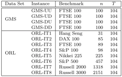
The second data set, hereafter referred to as ORL, is generated from the 8 benchmark instances for the index tracking problem currently belonging to the OR-Library (currently avail-able at http://people.brunel.ac.uk/~mastjjb/jeb/orlib/indtrackinfo.html). These in-stances consider the securities included in eight different stock market indices: the Hang Seng market index (related to the Hong Kong stock market), the DAX 100 (Germany), the FTSE 100 (United Kingdom), the S&P 100 (USA), the Nikkei 225 (Japan), the S&P 500 (USA), the Russell 2000 (USA) and the Russell 3000 (USA). The number of securities included in each instance ranges from 31, composing the Hang Seng index, to 2151, composing the Russell 3000 index. For each security, 291 weekly prices are provided in the original data set. Starting from this data set, we generate 8 instances consisting of the same number of in-sample and out-of-sample observations considered in data set GMS. Specifically, we used the first 105 prices in each instance to compute the rate of return of security j in scenario t, using the formula mentioned above whereqjtis taken equal to the (t+1)-th price provided in the original benchmark instance.
Table 1 summarizes the main characteristics of all the tested instances.
Data Set Instance Benchmark n T
GMS
GMS-UU FTSE 100 100 104 GMS-UD FTSE 100 100 104 GMS-DU FTSE 100 100 104 GMS-DD FTSE 100 100 104
ORL
ORL-IT1 Hang Seng 31 104 ORL-IT2 DAX 100 85 104 ORL-IT3 FTSE 100 89 104 ORL-IT4 S&P 100 98 104 ORL-IT5 Nikkei 225 225 104 ORL-IT6 S&P 500 457 104 ORL-IT7 Russell 2000 1318 104 ORL-IT8 Russell 3000 2151 104
Table 1: The main characteristics of the tested data sets.
To achieve some in-depth insights on the effectiveness of the proposed optimization models, and on the impact of the real features described above, we solved the OR model, the EOR model, as well as their extensions obtained adding constraints (27)–(34), on all the aforemen-tioned instances. From now on, the MILP models representing the extensions of OR and EOR models obtained adding Real Features (RF) are identified as OR-RF model and EOR-RF model, respectively. In the latter two models, parameter K in the cardinality constraint is set equal to 20 for all the instances in data set GMS. For data set ORL, K is set equal to 10 in the experiments concerning the 4 smallest instances (from ORL-IT1 to ORL-IT4), and to 20 for all the remaining test instances. Furthermore, we set parameters ǫj = 0.01 and ∆j = 0.15, for
j= 1, . . . , n.
The four optimization models were solved for 7 different values of the parameter α. Specif-ically, we set α equal to 0, 1%, 2%, 5%, 8%, 10% and 15% on a yearly basis (corresponding to values 0, 1.91371∗10−4, 3.80892∗10−4 9.38713∗10−4, 1.481116∗10−3, 1.834569∗10−3 and
2.691345∗10−3, on a weekly basis, respectively).
Finally, we set to 1 hour (3600 seconds) the threshold time to solve each instance. If the solver did not terminate within the allowed time, then the best feasible solution found was used to compute the performance measures reported in the following tables.
4.2 Evaluating the performance of the optimal portfolios
In this section, we comment on the main characteristics and the performance of the optimal portfolios selected by the proposed optimization models.
Table 2 provides in-sample and out-of-sample statistics for the OR and the OR-RF models, when solving the instances in the GMS data set. As mentioned above, each instance was solved for different values of µα. The first two columns of the table show the name of the instance
and the value of µα used, expressed in percentage and on yearly basis. Notice that, for each
instance, the first value of µα corresponds to α= 0, i.e., the figure reported is the mean rate of
return of the market indexµI. The main section of the table consists of two parts: the left-hand
out-of-sample period (yt > rIt %), the average portfolio rate of return in percentage and on
yearly basis (rav %), and the semi-standard deviation (s-std) computed compared to the market
index return as
q 1 52
P52
t=1(yt−rtI)2−. Finally, the last column with headerSortino Index reports
the average excess return divided by the semi-standard deviation s-std, where the excess return is measured from the mean return of the market index. For each instance, the average of each performance measure, computed over all the different values of µα, is reported in the last line.
The same set of statistics is reported in Table 3 for the EOR model and its extension EOR-RF for the instances of the GMS data set, while the figures in Tables 4 and 5 refer to the instances in the ORL data set.
We begin the in-sample analysis considering some characteristics of the optimal portfolios selected by the models without real features. As far as the number of securities composing the optimal portfolios is concerned, the EOR model tends to be more diversified than that selected by the OR model. The EOR model tends also to select portfolios with a better composition than those of OR model. This is especially true if we look at statistic Max %. Indeed, in almost all the instances the maximum share of the optimal portfolio found by the OR model is considerably larger than the corresponding one selected by the EOR model. Notice that in some instances (e.g., see the figures for instances GMS-DU and ORL-IT5 in Tables 2 and 4, respectively) statistic Max % for the portfolios found by the OR model is larger than 56 %, independently of the value of µα, while the same statistic for the EOR model is always smaller
than 15.3 % (see the figures reported in Tables 3 and 5). The above limitations of the portfolios selected by the OR model may be mitigated by the introduction of the real features described in 3.5. In both models, the number of securities composing the optimal portfolios often decreases as the value ofµα increases.
Computing times are negligible for all instances solved by the OR and EOR models. As expected, including real features in the optimization models makes their solution more time consuming, and, in particular, the smaller the value ofα, the larger the computing times (this is evident looking at the figures shown in Table 3 for the EOR-RF model and at those concerning the first 4 instances in Table 5). Note that, in some cases, computing times reach the imposed threshold time. We investigated further on this point removing the time limit of 3600 seconds and solving again all the instances not solved to optimality within such a time threshold. We found that the solutions obtained in the time limit are indeed the optimal ones, with the exception of the solution found by the EOR-RF model for instance ORL-IT6 setting µα = 0.4107 whose
percentage gap from the optimal solution is 0.78 %. Hence, we conclude that for those instances CPLEX is able to find the optimal (or near-optimal) solution relatively quickly, spending an excessive amount of computing time only to prove optimality.
corresponding values for the EOR-RF model).
Even though the above statistics enable us to give a synthetic measure of the out-of-sample performance of the portfolios, they do not provide an information of the portfolio performance over time. To this aim, in Figures 3-5 we analyze and compare the portfolio behavior in terms of cumulative returns. Cumulative returns of the corresponding market index are included in the pictures as terms of comparison. This representation allows a clear and complete comparison among the portfolios selected by the different optimization models, as well as a direct perfor-mance evaluation compared to the market index. To the sake of brevity, we decided to only report in the present paper the results concerning a subset of the tested instances and obtained by setting α= 0%, 2%, and 5% on yearly basis. The complete set of results for all the instances is provided as electronic supplementary material.
In Figures 3 and 4 we present the cumulative returns for the benchmarks and the portfo-lios selected by the OR model (upper left panel), the OR-RF model (upper right), the EOR model (lower left), and the EOR-RF model (lower right) in the instances UU and GMS-UD, respectively. In both figures the portfolios optimized by means of the EOR model clearly outperform those selected by the OR model. Indeed, in approximately the first half of the out-of-sample period depicted in Figure 3, all the portfolios selected by the OR model yield cu-mulative returns that fall below that of the benchmark. Subsequently, they perform similarly to the market index for some ex-post realizations, and, finally, they yield worse cumulative returns in the last weeks (especially the portfolio selected by settingαequal to 5%). On the other hand, the portfolios selected by the EOR model track very closely the behavior of the benchmark over almost the whole out-of-sample period, slightly outperforming the cumulative returns yielded by the market index in some of the realizations near the end of the period. The prevalence of the EOR model compared to the OR model is even more evident in Figure 4. The portfolios selected by the OR model show quite unstable cumulative returns. All these portfolios outperform the market index at the beginning of the ex-post period, yielding quite larger cumulative returns than the benchmark for some realizations, while their performance deteriorates significantly in the second part of the out-of-sample period. Conversely, the performance of the portfolios se-lected by the EOR model is very satisfactory. All the portfolios mimic closely the behavior of the benchmark, i.e., cumulative returns for the market index and the portfolios jointly increase or decrease in most of the ex-post realizations, while yielding larger cumulative returns. The higher volatility of the portfolios selected by the OR model than those found by the EOR model is confirmed by the larger values taken by static s-std and shown in Tables 2–5. Similar conclu-sions to those discussed above can be drawn comparing the cumulative returns yielded by the portfolios selected by the two models including real features. The only additional remark we draw is that, as mentioned above, the introduction of the real features often deteriorates the out-of-sample performance of the optimal portfolios.
on the performance of the optimal portfolios selected by setting α equal to 2% and 5%.
5
Conclusions and Future Directions
The index tracking problem represents one of the most studied and challenging problems in the financial literature of the last decades. However, more recently, researchers and practitioners seem to be more attracted by the enhanced indexation, where tracking is designed to outperform instead of simply mimic the market index performance. This has given rise to the Enhanced Index Tracking Problem (EITP) that aims at minimizing the index tracking error of a selected portfolio, while outperforming the market index.
In this paper we model the EITP by means of the Omega ratio. This is a recent performance measure that differs from the classical ones since it allows us to assess performance against a benchmark accounting for asymmetry in returns distribution. We propose two mathematical formulations for the EITP. In the first model the Omega ratio is computed with respect to a benchmark represented by the mean rate of return of the market index (OR model). The second model is obtained considering the portfolio optimization performance under multiple scenarios by substituting the mean rate of return of the benchmark market index with its random variable (EOR model). Both formulations, nonlinear in nature, are transformed into linear programming models and extended to include cardinality constraints and buy-in thresholds on investments giving rise to mixed integer linear programming models.
All optimization models were solved using CPLEX as solver. Extensive computational results on two different sets of benchmark instances have shown how the portfolios selected by the EOR model clearly outperform those found by the OR model in terms of out-of-sample performance. Furthermore, in most of the instances tested the portfolios optimized with the EOR model track very closely the behavior of the benchmark over the out-of-sample period, while yielding, sometimes, significantly larger returns. These results suggest that considering the market index as a random variable and its performance under all the scenarios is a valuable choice.
Finally, as future developments, one may consider a model extension with multiple levels of targets Rαi, where the downside deviations are defined as scaled (weighted) deviations for
several targets. Another interesting research direction is the study of possible extensions of the optimization models proposed in this paper in order to consider the possibility of rebalancing the portfolio composition, where transaction costs are paid. It is also interesting to investigate the performance of other optimization models where a different performance measure expressed as a ratio is adopted instead of the Omega ratio. As most of these ratios cannot be linearized, another possible development would be the design of efficient methods for their solution.
Acknowledgements
Research conducted by W. Ogryczak was partially supported by the National Science Centre (Poland) under the grant DEC-2012/07/B/HS4/03076 Construction of robust investment
te
of
C
on
tr
ol
&
C
om
p
u
tat
ion
E
n
gi
n
ee
ri
n
g
R
ep
or
t
2014–33
OR model OR-RF model
Instance Details In-Sample Out-of-Sample In-Sample Out-of-Sample CPU yt> Sortino CPU yt> Sortino
Name µα% Div. Min % Max % (sec.) rIt % rav% s-std Index Div. Min % Max % (sec.) r I
t % rav% s-std Index
GMS-UU
15.61 11 1.27 20.33 0.016 50.00 35.60 0.0172 -0.0827 11 1.30 15.00 0.140 48.08 33.28 0.0170 -0.1029 16.61 12 0.01 21.06 0.016 48.08 32.66 0.0182 -0.1011 12 1.00 15.00 0.140 48.08 35.22 0.0167 -0.0884 17.61 11 0.62 23.42 0.016 50.00 33.63 0.0183 -0.0931 12 1.00 15.00 0.156 48.08 35.84 0.0167 -0.0828 20.61 10 0.62 26.65 0.015 46.15 23.00 0.0221 -0.1498 11 1.10 15.00 0.093 48.08 33.64 0.0176 -0.0967 23.61 8 0.18 19.63 0.015 40.38 18.37 0.0237 -0.1704 10 3.19 15.00 0.109 46.15 30.42 0.0184 -0.1179 25.61 6 13.20 19.83 0.031 42.31 13.65 0.0252 -0.1916 9 2.84 15.00 0.125 42.31 24.79 0.0199 -0.1519 30.61 7 0.54 21.23 0.016 42.31 14.03 0.0257 -0.1855 10 1.00 15.00 0.172 42.31 21.28 0.0208 -0.1723
Average 9.29 2.35 21.74 0.018 45.60 24.42 0.0215 -0.1392 10.71 1.63 15.00 0.134 46.15 30.64 0.0182 -0.1161
GMS-UD
17.39 9 0.32 26.75 0.015 44.23 -30.79 0.0329 -0.1623 11 2.05 15.00 0.109 36.54 -32.01 0.0272 -0.2089 18.39 9 0.36 26.98 0.015 44.23 -31.40 0.0331 -0.1663 11 1.54 15.00 0.110 36.54 -32.38 0.0274 -0.2106 19.39 9 0.38 27.14 0.031 42.31 -31.62 0.0332 -0.1679 9 1.71 15.00 0.156 36.54 -33.22 0.0290 -0.2078 22.39 9 1.06 28.70 0.016 42.31 -30.67 0.0336 -0.1578 10 1.00 15.00 0.156 36.54 -34.39 0.0292 -0.2175 25.39 9 0.73 29.00 0.016 42.31 -32.24 0.0342 -0.1678 10 2.94 15.00 0.109 32.69 -35.03 0.0290 -0.2260 27.39 8 2.83 30.20 0.016 44.23 -31.16 0.0351 -0.1550 10 2.63 15.00 0.109 32.69 -34.42 0.0286 -0.2223 32.39 9 1.01 43.96 0.016 42.31 -33.77 0.0417 -0.1482 10 1.23 15.00 0.203 32.69 -41.96 0.0304 -0.2863
Average 8.86 0.96 30.39 0.018 43.13 -31.67 0.0348 -0.1608 10.14 1.87 15.00 0.136 34.89 -34.77 0.0287 -0.2256
GMS-DU
-21.15 12 0.38 75.47 0.015 51.92 13.08 0.0194 -0.1704 16 1.00 15.00 0.172 57.69 40.97 0.0166 0.0576 -20.15 12 0.03 77.50 0.015 51.92 11.85 0.0197 -0.1788 16 1.00 15.00 0.187 57.69 40.60 0.0166 0.0543 -19.15 12 0.84 74.70 0.015 50.00 14.21 0.0192 -0.1618 17 1.00 15.00 0.171 57.69 40.91 0.0165 0.0572 -16.15 12 0.17 75.22 0.015 50.00 14.94 0.0194 -0.1545 18 1.00 15.00 0.219 55.77 40.16 0.0164 0.0514 -13.15 12 0.61 74.23 0.015 51.92 15.50 0.0195 -0.1485 17 1.00 15.00 0.171 59.62 40.82 0.0164 0.0569 -11.15 12 0.21 73.28 0.016 53.85 15.91 0.0196 -0.1445 18 1.08 15.00 0.125 61.54 42.02 0.0160 0.0686 -6.15 11 0.09 64.24 0.016 53.85 21.38 0.0191 -0.1015 14 1.00 15.00 0.187 57.69 40.58 0.0163 0.0550
Average 11.86 0.33 73.52 0.015 51.92 15.27 0.0194 -0.1514 16.57 1.01 15.00 0.176 58.24 40.86 0.0164 0.0573
GMS-DD
-11.81 18 0.07 52.06 0.016 53.85 -1.50 0.0165 0.2855 20 1.26 15.00 0.125 67.31 -2.59 0.0128 0.3506 -10.81 20 0.02 51.10 0.016 53.85 -1.41 0.0164 0.2888 20 1.00 15.00 0.218 65.38 -2.83 0.0127 0.3494 -9.81 20 0.04 50.72 0.015 55.77 -1.23 0.0163 0.2919 20 1.00 15.00 0.203 65.38 -2.56 0.0128 0.3519 -6.81 18 0.13 48.99 0.016 55.77 -0.78 0.0160 0.3030 18 1.09 15.00 0.218 67.31 -1.02 0.0130 0.3700 -3.81 19 0.09 33.83 0.016 59.62 -0.33 0.0152 0.3239 19 1.00 15.00 0.250 65.38 -2.85 0.0129 0.3451 -1.81 19 0.25 22.72 0.015 59.62 -1.83 0.0142 0.3261 19 1.00 15.00 0.234 65.38 -3.16 0.0130 0.3366 3.19 15 0.71 26.79 0.016 63.46 -4.87 0.0138 0.2934 20 1.00 15.00 0.265 61.54 -4.15 0.0132 0.3179
[image:22.595.109.719.170.429.2]Average 18.43 0.19 40.89 0.016 57.42 -1.71 0.0155 0.3018 19.43 1.05 15.00 0.216 65.38 -2.74 0.0129 0.3459
Table 2: OR and OR-RF models: In-sample and out-of-sample statistics for the GMS data set.
te
of
C
on
tr
ol
&
C
om
p
u
tat
ion
E
n
gi
n
ee
ri
n
g
R
ep
or
t
2014–33
EOR model EOR-RF model
Instance Details In-Sample Out-of-Sample In-Sample Out-of-Sample CPU yt> Sortino CPU yt> Sortino
Name µα% Div. Min % Max % (sec.) rtI% rav% s-std Index Div. Min % Max % (sec.) r I
t % rav% s-std Index
GMS-UU
15.61 38 0.09 6.83 0.062 53.85 46.14 0.0057 0.0051 20 1.92 12.09 217.044 59.62 50.61 0.0071 0.0864 16.61 45 0.09 6.38 0.015 61.54 46.01 0.0052 0.0024 20 1.58 11.39 172.911 57.69 50.35 0.0072 0.0801 17.61 43 0.01 6.90 0.016 59.62 45.73 0.0053 -0.0048 20 2.19 12.25 46.832 57.69 48.29 0.0079 0.0394 20.61 33 0.10 9.10 0.015 50.00 46.89 0.0068 0.0191 20 2.14 14.95 4.415 53.85 45.61 0.0077 -0.0053 23.61 26 0.17 11.64 0.016 50.00 41.76 0.0087 -0.0644 20 1.00 12.48 0.265 50.00 44.72 0.0090 -0.0177 25.61 22 0.11 14.98 0.016 51.92 36.59 0.0109 -0.1169 20 1.27 15.00 0.234 48.08 36.14 0.0110 -0.1222 30.61 15 0.07 18.11 0.015 44.23 31.14 0.0135 -0.1530 14 1.00 15.00 0.172 44.23 30.29 0.0138 -0.1592
Average 31.71 0.09 10.56 0.022 53.02 42.04 0.0080 -0.0447 19.14 1.59 13.31 63.125 53.02 43.72 0.0091 -0.0141
GMS-UD
17.39 33 0.12 10.56 0.078 55.77 -0.20 0.0044 0.3781 20 2.09 11.12 198.058 55.77 -0.70 0.0052 0.3034 18.39 47 0.00 10.09 0.016 67.31 3.70 0.0046 0.5210 20 1.47 9.67 132.725 63.46 -1.61 0.0052 0.2697 19.39 46 0.04 9.98 0.016 65.38 3.35 0.0046 0.5075 20 1.39 10.16 89.326 59.62 -1.61 0.0053 0.2659 22.39 40 0.05 10.59 0.015 65.38 1.45 0.0043 0.4679 20 1.70 10.45 56.768 57.69 -2.78 0.0055 0.2141 25.39 33 0.01 9.76 0.016 59.62 1.37 0.0040 0.4942 20 1.39 11.59 7.473 51.92 -6.71 0.0064 0.0589 27.39 33 0.13 10.19 0.015 51.92 -7.23 0.0059 0.0460 20 1.15 11.02 3.993 42.31 -10.60 0.0071 -0.0613 32.39 28 0.15 11.35 0.016 42.31 -13.64 0.0097 -0.1140 20 1.52 12.11 1.638 40.38 -15.10 0.0103 -0.1387
Average 37.14 0.07 10.36 0.025 58.24 -1.60 0.0054 0.3287 20.00 1.53 10.88 69.997 53.02 -5.59 0.0064 0.1303
GMS-DU
-21.15 41 0.10 11.93 0.015 51.92 33.74 0.0030 -0.0217 20 1.00 11.70 10.686 48.08 31.18 0.0035 -0.1243 -20.15 39 0.11 11.36 0.016 59.62 34.84 0.0029 0.0327 20 1.15 11.78 6.334 48.08 31.47 0.0035 -0.1124 -19.15 37 0.10 10.03 0.016 50.00 33.10 0.0030 -0.0522 20 1.36 11.85 4.149 48.08 31.84 0.0034 -0.1000 -16.15 30 0.16 10.54 0.015 46.15 30.99 0.0035 -0.1334 20 1.08 10.54 2.371 50.00 30.74 0.0038 -0.1327 -13.15 27 0.07 12.03 0.016 46.15 31.69 0.0041 -0.0878 20 1.00 11.94 0.358 55.77 31.68 0.0044 -0.0836 -11.15 27 0.06 12.78 0.015 50.00 34.51 0.0042 0.0109 20 1.00 13.91 0.312 51.92 34.06 0.0043 -0.0042 -6.15 19 0.05 15.23 0.016 50.00 32.88 0.0052 -0.0362 17 1.00 14.40 0.281 48.08 33.69 0.0052 -0.0141
Average 31.43 0.09 11.99 0.016 50.55 33.11 0.0037 -0.0411 19.57 1.08 12.30 3.499 50.00 32.10 0.0040 -0.0816
GMS-DD
-11.81 37 0.23 9.92 0.078 53.85 -21.51 0.0048 0.0729 20 1.96 11.15 1064.514 48.08 -22.23 0.0049 0.0350 -10.81 47 0.14 10.72 0.016 38.46 -24.94 0.0040 -0.1259 20 1.64 10.53 625.780 48.08 -22.57 0.0050 0.0180 -9.81 44 0.07 10.07 0.015 46.15 -25.04 0.0041 -0.1303 20 1.89 11.88 601.225 51.92 -22.28 0.0052 0.0313 -6.81 42 0.02 9.78 0.016 53.85 -23.28 0.0042 -0.0205 20 1.37 10.36 155.220 51.92 -23.99 0.0070 -0.0379 -3.81 38 0.04 10.49 0.015 50.00 -21.64 0.0045 0.0698 20 1.96 10.33 37.549 57.69 -20.32 0.0066 0.0971 -1.81 34 0.27 10.42 0.016 57.69 -20.54 0.0058 0.1013 20 2.25 9.35 6.802 50.00 -20.47 0.0059 0.1019 3.19 30 0.18 10.85 0.016 59.62 -18.52 0.0070 0.1532 20 2.10 11.44 2.714 55.77 -19.81 0.0068 0.1115
[image:23.595.104.718.170.429.2]Average 38.86 0.14 10.32 0.025 51.37 -22.21 0.0049 0.0172 20.00 1.88 10.72 356.258 51.92 -21.67 0.0059 0.0510
Table 3: EOR and EOR-RF models: In-sample and out-of-sample statistics for the GMS data set.
st it u te of C on tr ol & C om p u tat ion E n gi n ee ri n g R ep or t 2014–33 ORL-IT1
49.60 4 9.84 49.14 0.016 59.62 12.76 0.0195 0.2895 8 1.76 15.00 0.078 55.77 -11.45 0.0116 0.0860 50.60 4 9.68 49.42 0.016 59.62 13.59 0.0195 0.2971 8 2.07 15.00 0.078 55.77 -11.55 0.0116 0.0839 53.60 4 7.97 50.77 0.016 57.69 16.90 0.0196 0.3240 7 11.09 15.00 0.093 55.77 -11.64 0.0115 0.0827 56.60 4 7.90 51.26 0.016 57.69 17.91 0.0196 0.3325 7 11.68 15.00 0.078 53.85 -11.86 0.0115 0.0785 58.60 4 4.05 53.76 0.016 55.77 25.91 0.0199 0.3904 7 12.07 15.00 0.078 53.85 -12.00 0.0115 0.0757 63.60 2 43.04 56.96 0.016 59.62 37.37 0.0207 0.4570 7 10.82 15.00 0.124 55.77 -11.61 0.0116 0.0826
Average 3.71 13.14 51.50 0.018 58.52 19.65 0.0197 0.3405 7.43 7.35 15.00 0.087 55.22 -11.64 0.0116 0.0824
ORL-IT2
7.16 13 0.32 21.55 0.031 53.85 11.43 0.0155 0.1261 10 5.00 15.00 0.265 51.92 11.59 0.0156 0.1274 8.16 13 0.10 22.15 0.015 51.92 10.09 0.0156 0.1107 10 5.00 15.00 0.375 51.92 11.64 0.0156 0.1277 9.16 12 0.34 23.19 0.016 53.85 9.71 0.0156 0.1062 10 4.38 15.00 0.234 51.92 12.35 0.0156 0.1360 12.16 11 1.47 29.03 0.016 53.85 5.35 0.0160 0.0548 10 2.85 15.00 0.171 48.08 9.02 0.0150 0.1028 15.16 12 0.56 31.79 0.016 55.77 4.62 0.0163 0.0457 10 2.36 15.00 0.156 48.08 9.09 0.0149 0.1042 17.16 12 0.51 31.62 0.031 55.77 3.61 0.0163 0.0343 10 1.78 15.00 0.172 50.00 9.22 0.0149 0.1055 22.16 9 2.21 37.21 0.016 50.00 4.17 0.0167 0.0395 9 6.01 15.00 0.156 46.15 8.72 0.0150 0.0991
Average 11.71 0.79 28.08 0.020 53.57 7.00 0.0160 0.0739 9.86 3.91 15.00 0.218 49.73 10.23 0.0152 0.1147
ORL-IT3
14.20 12 0.08 20.23 0.031 50.00 -10.22 0.0217 -0.0328 10 1.75 15.00 0.172 50.00 -8.55 0.0219 -0.0163 15.20 12 0.00 20.03 0.015 50.00 -10.03 0.0217 -0.0309 10 1.00 15.00 0.156 50.00 -8.69 0.0221 -0.0175 16.20 12 0.29 19.66 0.015 50.00 -9.97 0.0218 -0.0302 10 1.38 15.00 0.187 50.00 -8.83 0.0221 -0.0188 19.20 11 0.63 20.09 0.015 50.00 -9.48 0.0220 -0.0251 9 2.16 15.00 0.156 50.00 -7.91 0.0219 -0.0102 22.20 10 0.17 23.40 0.015 46.15 -9.33 0.0213 -0.0245 9 2.79 15.00 0.141 50.00 -7.51 0.0218 -0.0065 24.20 8 0.41 24.02 0.031 46.15 -8.46 0.0212 -0.0159 9 4.33 15.00 0.109 51.92 -6.38 0.0214 0.0043 29.20 7 3.86 27.55 0.015 44.23 -6.00 0.0208 0.0082 10 1.00 15.00 0.156 48.08 -4.22 0.0209 0.0253
Average 10.29 0.78 22.14 0.020 48.08 -9.07 0.0215 -0.0216 9.57 2.06 15.00 0.154 50.00 -7.44 0.0217 -0.0057
ORL-IT4
6.46 12 1.14 21.61 0.015 48.08 1.77 0.0205 -0.0342 10 4.27 15.00 0.187 50.00 0.64 0.0221 -0.0414 7.46 12 0.95 21.72 0.031 48.08 2.16 0.0204 -0.0307 10 4.32 15.00 0.234 50.00 0.36 0.0222 -0.0437 8.46 12 1.12 22.60 0.031 48.08 1.44 0.0213 -0.0359 10 3.99 15.00 0.203 50.00 0.23 0.0225 -0.0442 11.46 10 3.09 17.94 0.031 50.00 -0.34 0.0234 -0.0473 10 3.01 15.00 0.156 50.00 0.41 0.0228 -0.0422 14.46 10 0.90 23.72 0.031 50.00 -3.28 0.0248 -0.0677 10 2.11 15.00 0.109 48.08 0.97 0.0231 -0.0369 16.46 10 0.77 27.44 0.015 50.00 -3.72 0.0261 -0.0678 10 1.77 15.00 0.171 48.08 0.78 0.0232 -0.0383 21.46 6 2.51 36.10 0.015 51.92 -7.17 0.0322 -0.0767 10 4.46 15.00 0.188 48.08 3.03 0.0230 -0.0202
Average 10.29 1.50 24.45 0.024 49.45 -1.31 0.0241 -0.0515 10.00 3.42 15.00 0.178 49.18 0.92 0.0227 -0.0381
ORL-IT5
-0.88 4 9.81 56.52 0.031 46.15 -28.08 0.0225 -0.1526 9 1.00 15.00 0.187 48.08 -20.57 0.0162 -0.0942 0.12 4 9.96 59.60 0.031 48.08 -28.26 0.0229 -0.1522 8 3.47 15.00 0.141 48.08 -20.58 0.0163 -0.0943 1.12 4 10.02 59.45 0.016 48.08 -28.23 0.0228 -0.1520 8 3.64 15.00 0.140 48.08 -20.62 0.0163 -0.0949 4.12 5 2.83 70.04 0.031 46.15 -28.45 0.0242 -0.1456 8 4.33 15.00 0.140 48.08 -20.79 0.0163 -0.0971 7.12 4 2.78 87.83 0.031 46.15 -28.74 0.0266 -0.1354 8 2.82 15.00 0.141 44.23 -21.63 0.0166 -0.1078 9.12 3 3.11 90.62 0.031 46.15 -28.67 0.0272 -0.1321 8 1.45 15.00 0.140 40.38 -23.09 0.0172 -0.1247 14.12 2 10.73 89.27 0.031 46.15 -29.51 0.0275 -0.1386 9 2.93 15.00 0.281 42.31 -23.44 0.0175 -0.1279
Average 3.71 7.04 73.33 0.029 46.70 -28.56 0.0248 -0.1441 8.29 2.81 15.00 0.167 45.60 -21.53 0.0166 -0.1058
ORL-IT6
26.07 15 0.08 16.43 0.047 46.15 38.42 0.0291 0.0714 14 1.00 15.00 0.421 46.15 39.26 0.0284 0.0772 27.07 15 0.31 17.27 0.031 50.00 50.35 0.0290 0.1267 14 1.00 15.00 0.764 46.15 40.29 0.0283 0.0824 28.07 14 0.05 18.49 0.031 51.92 64.20 0.0291 0.1851 14 1.35 15.00 0.359 46.15 46.98 0.0279 0.1160 31.07 13 0.78 20.65 0.031 53.85 100.82 0.0297 0.3133 13 2.49 15.00 0.327 50.00 54.06 0.0290 0.1429 34.07 11 0.11 22.07 0.046 53.85 106.43 0.0302 0.3263 12 2.05 15.00 0.327 51.92 94.32 0.0291 0.2979 36.07 11 0.09 21.62 0.031 53.85 109.19 0.0303 0.3333 12 1.99 15.00 0.343 51.92 93.15 0.0291 0.2933 41.07 11 0.48 23.06 0.031 55.77 150.30 0.0318 0.4277 12 1.00 15.00 0.437 55.77 105.41 0.0291 0.3343
Average 12.86 0.27 19.94 0.035 52.20 88.53 0.0299 0.2548 13.00 1.55 15.00 0.425 49.73 67.64 0.0287 0.1920
ORL-IT7
9.22 46 0.06 13.58 0.093 53.85 34.39 0.0167 0.1747 20 1.74 15.00 3601.438 55.77 21.10 0.0192 0.0470 10.22 49 0.10 13.47 0.093 53.85 36.57 0.0166 0.1948 20 1.70 15.00 3602.718 53.85 28.83 0.0162 0.1293 11.22 49 0.02 13.57 0.093 53.85 36.78 0.0165 0.1968 20 1.00 12.22 3602.717 53.85 18.01 0.0185 0.0218 14.22 47 0.15 14.43 0.078 53.85 36.03 0.0160 0.1973 20 1.18 15.00 3602.171 59.62 32.08 0.0180 0.1433 17.22 54 0.05 10.68 0.093 51.92 27.88 0.0162 0.1205 20 1.19 12.81 3603.091 57.69 31.56 0.0176 0.1425 19.22 54 0.03 13.12 0.094 55.77 32.54 0.0157 0.1683 20 1.02 12.51 3602.982 53.85 28.43 0.0188 0.1083 24.22 46 0.05 8.64 0.093 51.92 32.21 0.0163 0.1592 20 1.22 12.82 3602.468 48.08 22.09 0.0199 0.0534
Average 49.29 0.07 12.50 0.091 53.57 33.77 0.0163 0.1731 20.00 1.29 13.62 3602.512 54.67 26.01 0.0183 0.0923
ORL-IT8
23.36 57 0.01 10.75 0.140 51.92 24.06 0.0194 0.0028 20 1.40 13.24 3602.936 48.08 30.81 0.0222 0.0485 24.36 56 0.01 11.17 0.156 53.85 25.58 0.0194 0.0149 20 1.78 12.82 3602.390 46.15 36.25 0.0201 0.0927 25.36 55 0.05 12.59 0.156 53.85 25.11 0.0194 0.0112 20 1.41 11.91 3602.842 51.92 28.37 0.0218 0.0329 28.36 48 0.09 11.89 0.156 51.92 28.70 0.0194 0.0394 20 1.43 10.60 3602.046 53.85 32.56 0.0213 0.0628 31.36 47 0.04 8.64 0.156 46.15 31.92 0.0198 0.0627 20 1.62 10.77 3601.968 51.92 33.55 0.0214 0.0692 33.36 47 0.06 8.18 0.156 46.15 32.90 0.0206 0.0672 20 1.07 8.99 3600.190 50.00 22.84 0.0238 -0.0057 38.36 43 0.00 7.75 0.156 51.92 36.02 0.0218 0.0841 20 1.00 11.60 1115.433 51.92 44.23 0.0227 0.1310
[image:24.595.106.764.68.544.2]