CKY Parsing with Independence Constraints

(1)

CKY Parsing With Independence Constraints

Joseph Irwin

Graduate School of Information Science Nara Institute of Science and Technology

Nara, Japan

[email protected]

Yuji Matsumoto

Graduate School of Information Science Nara Institute of Science and Technology

Nara, Japan

[email protected]

Abstract

The CKY algorithm is an important com-ponent in many natural language parsers. We propose a novel type of constraint for context-free parsing called independence constraints. Based on the concept of in-dependence between words, we show how these constraints can be used to reduce the work done in the CKY algorithm. We demonstrate a classifier which can be used to identify boundaries between indepen-dent words in a sentence using only sur-face features, and show that it can be used to speed up a CKY parser. We investigate the trade-off between speed and accuracy, and indicate directions for improvement.

1 Introduction

The CKY algorithm is anO |G|n3_dynamic

pro-gramming algorithm for finding all of the possi-ble derivations of a sentence in a context-free lan-guage. Its complexity depends on both the sen-tence length nand the size of the grammar |G|. Methods for improving parsing accuracy typically increase the size of the grammar (Klein and Man-ning, 2003; Petrov and Klein, 2007) or even the exponent of n (Eisner and Satta, 1999). More powerful “deep” grammar formalisms multiply the computational complexity even more (Banga-lore and Joshi, 1999).

A common technique for speeding up such parsers is coarse-to-fine parsing, where input is first parsed using a much simpler (and thus smaller) grammar, and the content of the chart is then used to constrain the search over the fi-nal grammar (Torisawa et al., 2000; Charniak and Johnson, 2005; Petrov and Klein, 2007). Even with a much smaller grammar, the CKY algorithm may be expensive—Roark et al. (2012) report that the initial CKY step in the Berkeley Parser takes half of the total parse time.

S

NP

DT

0This1

VP

VB

is2

NP

DT

an3

NN

example4

.

[image:1.595.340.491.205.340.2]

.5

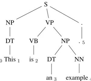
Figure 1: In this tree ‘This’ and ‘is’ are indepen-dent, while ‘is’ and ‘an’ are not.

Other techniques can be used to prune cells in the chart. Roark et al. (2012) use a finite-state model to label words that do/don’t begin/end spans, and skip cells that don’t satisfy the labels. Bodenstab et al. (2011) directly apply a clas-sifier to each cell to decide how many spans to keep. Both approaches reduce the work done by the parser while preserving accuracy.

We propose a novel type of top-down constraint for a CFG parser that we call independence con-straints, described in Section 2. In Section 3 we show how the CKY algorithm can be easily modi-fied to accommodate these constraints, and in Sec-tion 4 we describe a classifier which can provide the constraints to a parser. We integrate the con-straints into the Stanford Parser CKY implemen-tation and show the results in Section 5.

2 Independence Constraints

We propose a concept we call independence. Given a sentences=w1w2. . . wnand a context-free derivation (parse tree) t of s, words wi and wi+1areindependentif every node intthat

dom-inates both wi and wi+1 also dominates w1 and wn. Furthermore, ifwiandwi+1are independent,

then ∀j, k s.t. j ≤ iandk > i, wj andwk are

(2)

independent. Less formally, if the children of the top node of a parse tree were split into separate subtrees, two words are independent if they would end up in different subtrees.

An example is shown in Figure 1. Here, ‘This’ and ‘is’ are independent, as are ‘example’ and ‘.’. The independent spans are (‘This’), (‘is’, ‘an’, ‘ex-ample’), and (‘.’), with boundaries 1 and 4. The in-dependent spans and inin-dependent span boundaries can be derived straightforwardly from the defini-tion of independent words: the locadefini-tions between consecutive words which are independent are the independent span boundaries, and the independent spans are simply the spans in between consecutive boundaries.

3 Modifying The CKY Algorithm With Independence Constraints

Conceptually, if a CKY parser knows the locations of the independent span boundaries for a sentence, it can perform the normal CKY algorithm for each independent span separately, and simply join the spans at the top of the tree to finish the parse, thereby avoiding work which would otherwise be done while still obtaining the desired 1-best parse. Two issues make the task more complicated than this.

The first complication is that if we assume that the independent boundaries will be identified au-tomatically, we must allow for errors. If a loca-tion which is not an independent span boundary is given as one, the parser will make an error it would not have otherwise. On the other hand, if a loca-tion which is an independent span boundary is not marked as such, the parser may account for this at the cost of not achieving the minimum computa-tion possible. By allowing for this second type of error, the algorithm is made more robust, and al-lows the independent boundary identification step to prioritize precision over recall to lessen negative impact on the parser’s accuracy.

The second issue is caused by the binarization of the context-free grammar used in the CKY al-gorithm. Because the CKY algorithm requires a binary grammar, any rules in the original gram-mar that have more than two symbols on the right-hand side must be converted into a sequence of bi-nary rules. The extra rules created in this process are called incomplete1_{rules. The topmost span in}

1_{E.g., if a rule}_A _→ _BCD_becomes_@

[image:2.595.330.502.64.151.2]

BC → BCand A→@BCD, then the former isincompleteand the latter is

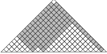
Figure 2: Example of a CKY chart with indepen-dence constraints. In the gray cells the modified algorithm will only loop over incomplete rules.

particular will usually need to be constructed in several steps, applying multiple incomplete rules before creating a complete span. If the grammar rules are always binarized from the left (right), then only cells on the left (right) edge of the chart can affect the top span; however, the grammar used in our parser is binarized “head-outward” (Klein and Manning, 2003), which means that po-tentially any cell in the chart can be used to create the top span.

The combination of these two issues means that in order to correctly parse a sentence when an dependent span boundary is missing from the put the modified CKY algorithm must process in-complete rules even at positions in the chart that cross a boundary. Thus in the modified algorithm, cells which do not cross an independent bound-ary are processed normally, and in cells which do cross a boundary the algorithm will avoid loop-ing over complete binary rules.2 _{Figure 2 shows}

an example CKY chart where boundary-crossing cells are colored gray.

3.1 How much work can we expect to save? The core of the CKY algorithm is shown in Al-gorithm 1. For our purposes, we can consider the amount of work done in the CKY algorithm to be the number of binary edges visited in the inner loop (lines 4-10). For each cell the algorithm it-erates over the binary rules in the grammar, calcu-lating the probability of the left-hand-side at each split point. The number of these binary edges is

complete.

2_{While boundary-crossing cells depend on non-crossing}

(3)

1 for1≤i≤ndo

2 T_i,i₊₁ ← {A|A→a∈G∧w_i=a} 3 end

4 for2≤j≤ndo

5 for1≤i≤n−j+ 1do 6 fori < k < i+jdo

7 T_i,i₊_j ← {A|A→BC∈

G∧B ∈Ti,k∧C∈Tk,i+j}

8 end

9 end 10 end

Algorithm 1: The CKY algorithm. Ti,j is the cell corresponding to wordswi. . . wj−1.

|G|

n3 6 −

n 6

(1)

The amount of work saved depends on the num-ber and locations of the independent span bound-aries, as well as the proportion of complete rules in the grammar, denoted |Gcomp|

|G| . We can consider

two idealized scenarios: a) one boundary at n K, and b) K −1 boundaries at _Kn,2_Kn, . . . ,(K−_K1)n, whereKis an integer1< K < n.

For the first case, the ratio of work saved ap-proaches

|Gcomp| |G|

3 K −

3 K2

(2)

as n grows. This limit converges quickly for

n ≥ 10. If we approximate |Gcomp|/|G|as 0.5 (for the grammar used by the parser in Section 5, it is≈.54), then forK = 2,3,4, . . ., the values are

3

8,13,323 , . . . Intuitively, for one boundary, the best

location is exactly in the center of the sentence, and the upper limit on how much work is saved is about 37%.

For the case ofK−1boundaries equally spaced, the ratio is

|Gcomp| |G|

K2₋₁

K2 (3)

The values forK = 2,3,4, . . . are3₈,4₉,15₃₂, . . .

Clearly, the smaller pieces a sentence can be di-vided into the less work the parser will do; how-ever, realistically most sentences will not have a large number of independent spans, and they will not be equal in length. We might takeK = 3 as best-case estimate, giving us about 44%. Thus we can guess that a parser will be able to save around

Local Features

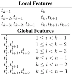
tk−1 tk tk−2, tk−1 tk, tk+1 tk−3, tk−2, tk−1 tk, tk+1, tk+2

Global Features

tl

i 1≤i < k−1 tl

i, tli+1 1≤i < k−2 tl

i, tli+1, tli+2 1≤i < k−3 tl

i k≤i < n−1 tl

i, tli+1 k≤i < n−2 tl

[image:3.595.344.491.62.212.2]

i, tli+1, tli+2 k≤i < n−3

Table 1: Feature templates. kis the boundary po-sition,tkis thekth POS tag (level 0), andtliis the ith POS tag in thel-level POS tag sequence.

35-45% of the work it does in the CKY algorithm loop by using independence constraints.

The derivations of Equations 1-3 are shown in Appendix A.

4 Classifying Independent Span Boundaries

In order to use independence constraints in a parser, we need to be able to identify boundaries between independent words in a sentence using only surface features (words and part-of-speech tags). We created a binary classifier which, given a POS-tagged sentence and a position between two words, decides whether those two words are inde-pendent or not. Our classifier currently uses only POS tags as features. We usedopal(Yoshinaga and Kitsuregawa, 2010), a tool for fast online clas-sification, to train and test the models, training on sentences from Penn Treebank section 02-21 and testing on section 22. We set opal to use the passive-aggressive perceptron update, and output probabilities in order to use a threshold to trade off precision and recall.

4.1 Features

(4)

Features #feats Acc Prec Rec F1 F0.5 TP FP FN TN

p 37001 93.71 80.73 70.49 75.27 78.45 3679 878 1540 32320

P0 33167 87.16 51.69 83.98 63.99 55.99 4383 4097 836 29101

p,P0 70168 95.21 87.38 75.65 81.09 84.75 3948 570 1271 32628

p,P1 37055 94.81 78.38 85.38 81.73 79.69 4456 1229 763 31969

p,P2 39336 95.34 84.25 80.76 82.47 83.53 4215 788 1004 32410

p,P3 46861 95.04 89.47 71.95 79.76 85.31 3755 442 1464 32756

p,P0,P1 70222 95.48 88.95 76.16 82.06 86.06 3975 494 1244 32704

p,P0,P2 72503 95.09 88.28 73.60 80.27 84.89 3841 510 1378 32688

p,P0,P3 80028 94.84 88.81 70.99 78.91 84.56 3705 467 1514 32731

p,P1,P2 39390 95.27 80.99 85.21 83.04 81.80 4447 1044 772 32154

p,P1,P3∗ 41553 95.44 89.05 75.74 81.86 86.03 3953 486 1266 32712

[image:4.595.71.508.61.240.2]

p,P0,P1,P2,P3 82417 95.35 86.89 77.49 81.92 84.83 4044 610 1175 32588

Table 2: Results of classifier using different combinations of features. (∗_{Final feature configuration.)}

Lvl0 Lvl1 Lvl2 Lvl3 Lvl0 Lvl1 Lvl2 Lvl3

NN N N N CD X X #

NNP N N N -LRB- X X B

NNPS N N N -RRB- X X B

NNS N N N DT X X D

PRP N N N PDT X X D

VB V V V PRP$ X X D

VBD V V V WP$ X X D

VBG V V V JJ X X J

VBN V V V JJR X X J

VBP V V V JJS X X J

VBZ V V V -RQ- X X Q

, X , , -LQ- X X Q

. X . . RB X X R

: X : : RBR X X R

CC X C C RBS X X R

IN X I I EX X X X

RP X I I FW X X X

TO X T T LS X X X

WDT X W W MD X X X

WP X W W POS X X X

WRB X W W SYM X X X

# X X # UH X X X

$ X X #

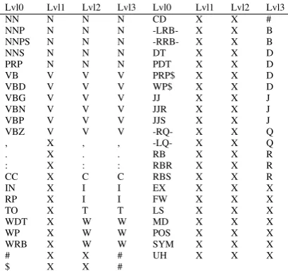
Table 3: For each POS level, the original tag is replaced with the corresponding value.

4.2 POS Level

In previous unpublished work on a similar task, we found that heuristically transforming the POS tag sequence to create additional features can be ben-eficial. We refer to these transformations asPOS levels. In this classifier we implemented three lev-els, in addition to the original POS tags as level 0.

We show all levels in Table 3. Each level spec-ifies a value by which each level 0 tag is replaced during the transformation. The motivation behind each transformation is roughly as follows: level 1 is meant to capture clause nuclei; level 2 is further intended to show boundaries between clauses; and level 3 expands almost all the way back to the orig-inal tags, but with some distinctions erased, mostly to reduce the number of features.

4.3 Which Features Are Useful?

In order to find the best configuration of features for the classifier, and to evaluate the proposed POS levels, we tested the classifier using several differ-ent combinations. Selected results are shown in Table 2. In the "Features" column, pdenotes the local features, and Pl denotes the global features from POS levell.

There are several things worth noting in these results. First, neither local nor global features are sufficient alone; it appears that local features pro-mote precision, while global features propro-mote re-call. Second, examining the cases where global features are limited to a single POS level, it is ap-parent that each POS level has a different effect on precision and recall, thus confirming that the clas-sifier is able to extract different signals from the different POS levels, as intended. Finally, combin-ing all POS levels together actually reduces accu-racy, possibly because the features are highly cor-related (although see the discussion of the kernel classifier).

4.4 Results

To avoid degrading the accuracy of the parser as much as possible, we selected the feature config-uration based on F0.5 score, a measure which

fa-vors precision over recall. We chosep, P1, P3over

p, P0, P1 because the former had a slight edge in

precision and fewer features.

[image:4.595.78.283.280.472.2]

(5)

thresh-Features Threshold Acc Prec Rec F1 F0.5 TP FP FN TN

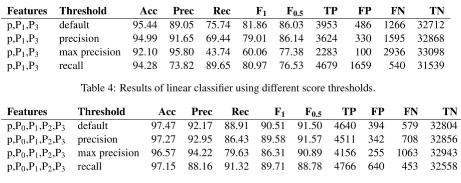
p,P1,P3 default 95.44 89.05 75.74 81.86 86.03 3953 486 1266 32712

p,P1,P3 precision 94.99 91.65 69.44 79.01 86.14 3624 330 1595 32868

p,P1,P3 max precision 92.10 95.80 43.74 60.06 77.38 2283 100 2936 33098

[image:5.595.71.531.58.241.2]

p,P1,P3 recall 94.28 73.82 89.65 80.97 76.53 4679 1659 540 31539

Table 4: Results of linear classifier using different score thresholds.

Features Threshold Acc Prec Rec F1 F0.5 TP FP FN TN

p,P0,P1,P2,P3 default 97.47 92.17 88.91 90.51 91.50 4640 394 579 32804

p,P0,P1,P2,P3 precision 97.27 92.95 86.43 89.58 91.57 4511 342 708 32856

p,P0,P1,P2,P3 max precision 96.57 94.22 79.63 86.31 90.89 4156 255 1063 32943

p,P0,P1,P2,P3 recall 97.15 88.16 91.32 89.71 88.78 4766 640 453 32558

Table 5: Results of polynomial classifier using different score thresholds.

old did slightly improve in F0.5.

4.5 Efficiency of the Classifier

The efficiency of the classifier is as important as the accuracy—it doesn’t matter how much time is saved during parsing if it takes even longer to run the classifier.opaltakes less than half a sec-ond to run on the instances from section 22; how-ever, the instances are created by a Python script, which is not very optimized. This script takes about 100 seconds to run on the machine described in Section 5.1. While this time is already less than the time saved in the parser (see Section 5.2), it could be significantly reduced by re-implementing in Java or even C++. Thus the potential gains of-fered by this approach are not just theoretical.

4.6 Polynomial Kernel

For comparison with the linear classifier, we trained another classifier using a polynomial ker-nel (with degree 3) with all the features. The re-sults are shown in Table 5. The polynomial ker-nel improves over the linear classifier in accu-racy by 2%, in precision by 3 points, and in re-call by just over 13 points. This suggests that there is a large potential for improving the linear classifier by adding conjunctive features. Alterna-tively, there are methods for effectively lineariz-ing a kernel-based classifier, e.g. (Kudo and Mat-sumoto, 2003; Isozaki and Kazawa, 2002). Cur-rently, the polynomial classifier takes over 2 hours to run on section 22 (training the model took al-most 4 days).

5 Parsing With Independence Constraints

In order to demonstrate use of the independent constraints in a parser, we modified the CKY parser included in the Stanford Parser distribu-tion to accept independent span boundaries as con-straints and to use the modified CKY algorithm described above. Our modifications are:

• after reading in the grammar, index the in-complete binary rules

• read in the file containing the boundaries out-put by the classifier from the previous section • for each CKY cell, if the cell spans a bound-ary then loop over just the incomplete binbound-ary rules

• if at the end of the CKY loop a parse was not successful, then loop again over just the cells which span a boundary and process all of the binary rules

• output the total number of times entering the inner loop as well as the number of times the parser failed

5.1 Experimental Setup

We used the modified Stanford Parser described above, with an unlexicalized grammar3 _extracted

from the WSJ sections 02-21, and evaluated its performance on section 22 using output from the classifier as constraints. For the baseline, the 3_{The grammar was extracted using the Stanford}

(6)

Parser Time (s) Speedup # Binary Edges F1 Parse Failures

baseline 1558 - 1.75×1010_{(100%) 85.85} ₀

linear 1283 (+100) 1.21× (1.12×) 1.08×1010_(62%) _{83.71 (-2.14)} ₁₅

poly 1106 (+2h) 1.41× (.19×) 9.74×1009_(56%) _{84.85 (-1.00)} ₆

[image:6.595.70.502.62.131.2]

oracle 1016 1.53× 8.47×1009_(48%) _{86.71 (+0.86)} ₄

Table 6: Results of parsing with independence constraints. Results for both linear and polynomial clas-sifiers are shown, as well as for the gold independent span boundaries. The times in parentheses are the classifier run times.

parser was given null constraints. The accuracies and times shown are those reported by the Stan-ford Parser.

All experiments were run on a DELL Precision 690, with 8 cores and 32G of RAM. Unless other-wise noted multiple processes were run in parallel, and times reported were not averaged over multi-ple runs. Since we saw significant variation of up to 10%, the times should be taken with a grain of salt. The computation done in the CKY algorithm is measured in the number of binary edges visited in the inner loop. A binary edge is a tuple of a span (begin & end), a binary ruleA→BC, and a split point (the position whereBandCmeet).

5.2 Results

The results of running the parser on section 22 us-ing the linear classifier from Section 4.4 are shown in Table 6. The table shows the total time taken, the total times entering the inner loop, the F1 and

difference from the baseline, and the number of times the parse failed using the constraints. The parser with independence constraints saves 38% of the computation inside the CKY loop over the baseline, corresponding to about 20% reduction in total parse time (12% if the running time of the classifier is included), at the cost of a 2-point drop in F-score. Detailed results of further exper-iments with various thresholds on sentence length and classifier score are shown in Appendix B. 5.3 Polynomial Kernel

A difference of 2 F1 score is not small, but on the

other hand it is about by how much the unlexi-calized Stanford Parser trails the Collins parser, for example. However, as shown above in Sec-tion 4.6, there is room to improve the linear classi-fier through conjunctive features. As an indication of an upper bound of the achievable performance, we tried using the output of the kernel classifier in the parser as above, while acknowledging that at present the time needed to produce the classifier

Parser Time(s) Speedup F1

baseline 1538 85.54

linear 1106 1.39× 83.55 (-1.99) (+100) (1.28×)

poly 1040 1.48× 84.57 (-0.97)

Table 7: Results of parsing WSJ section 23.

output dwarfs the time needed to actually parse the test data.

The results of running the parser on section 22 with the polynomial classifier output are shown with the previous results in Table 6. With the more accurate classifier, the parser is able to re-duce the necessary computation even further, by 44%, while losing less accuracy.

5.4 Gold Independent Span Boundaries For another comparison, we tested the parser using the gold independent span boundaries. The results for section 22 are shown in Table 6. The number of binary edges visited is cut in half, and parsing accuracy is improved by almost 1 point. It is inter-esting to note that the parser was unable to parse 4 sentences with the gold constraints (the grammar only allowed a parse that violated the gold bound-aries).

5.5 WSJ Section 23

To compare with previous work on parsing using the Penn Treebank, we show the time and accuracy for parsing section 23, using both linear and ker-nel classifier output along with the baseline parser in Table 7. The times reported are the average of three runs each. Because there was significant variation in parse time when multiple processes were run in parallel, for these results only one pro-cess was run at a time. The results parallel those shown on the development data.

[image:6.595.309.524.195.266.2]

(7)

due to differences in parser (their parsers use beam search variants of CKY and coarse-to-fine prun-ing) and grammar (they used the Berkeley latent variable grammar and a lexicalized grammar).

6 Related Work

There are several strains of research related to adding constraints to the CKY chart. (Roark et al., 2012) describes an approach using finite-state taggers to decide whether each word in a sentence begins or ends a multiword constituent and has a unary span or not. They show that their tagger is able to achieve very high precision, reducing parse time without negatively affecting accuracy.

(Bodenstab et al., 2011) proposes a classifier which directly decides for each cell in the chart how many constituents should be created. Their parser uses beam search with a FOM and a beam for each chart cell.

Like these approaches, our method uses a clas-sifier to avoid doing work in certain chart cells. While not completely orthogonal, we believe our independence constraints are complementary. A single decision by our classifier closes a large swath of cells based on the global structure, while their methods make local decision using local in-formation. The high accuracy of their classifiers shows the necessity of improving our model.

(Yarmohammadi et al., 2014) proposes a con-cept of ‘hedge’ parsing, where only spans below a certain length are allowed, and show how this reduces the computation done by the CKY al-gorithm. Their system does not create spans of length larger than the threshold and thus doesn’t follow the original treebank annotation, while our approach is able to return the original gold parse tree, provided that the classifier does not output a false positive. Their approach of segmenting a sentence before parsing is essentially the same as ours, but they segment based on a maximum span length and their classifier is based on a finite-state sequence model.

There is some previous research using clause boundaries to constrain dependency parsers (Ohno et al., 2006; Husain et al., 2011; Kim and Lee, 2004). This is more linguistically motivated than our constraints; indeed, the approaches appear to rely on processing specific to each language. It is difficult to compare with these results directly; however, although only (Ohno et al., 2006) re-ported parse times, all three papers rere-ported

im-proved accuracy.

7 Conclusions

We have proposed a property ofindependence be-tween words in a sentence, and shown how to use this property to create top-down constraints which can be used to reduce the computation done by the CKY algorithm. We demonstrated two classi-fiers for identifying boundaries between indepen-dent words given a sentence with only surface fea-tures, a linear classifier which is fast but less ac-curate, and a classifier with a polynomial kernel which is much more accurate but very slow. We then showed a significant improvement in speed over a strong baseline CKY parser by using the output of these classifiers to create top-down con-straints at the cost of some accuracy.

Although the loss of accuracy when using the linear classifier is currently uncomfortably large, there are several possible avenues for improve-ment. The performance of the kernel classifier indicates that there is room for improvement by manually adding conjunctive features to the linear classifier or using a method to automatically lin-earize the model. Features based on words as well as POS tags may also be beneficial. Changing the model itself to, e.g., a sequence model might also help. However, the current approach has several weaknesses which should be addressed by future research.

First, the top-down nature of the independence constraints does not make a natural fit with the bottom-up CKY algorithm. In particular, the pres-ence of incomplete rules in the grammar combined with the bottom-up search means that the parser still ends up doing some computation to create spans which violate the constraints, even though it is prevented from completing such a span.

Second, the pipelined nature of the classifier means that it only has access to POS tags and in particular is not able to make use of informa-tion generated as the parser processes lower-level spans. Tighter integration of the classifier into the parser may be beneficial to both.

(8)

References

Srinivas Bangalore and Aravind K Joshi. 1999. Su-pertagging: An Approach to Almost Parsing. Com-putational Linguistics, 25:237–265.

Nathan Bodenstab, Aaron Dunlop, Keith Hall, and Brian Roark. 2011. Beam-Width Prediction for Ef-ficient Context-Free Parsing. InProceedings of the 49th Annual Meeting of the Association for Compu-tational Linguistics, pages 440–449, Portland, Ore-gon. Association for Computational Linguistics. Eugene Charniak and Mark Johnson. 2005.

Coarse-to-fine n-best parsing and maxent discriminative reranking. InACL 2005.

Jason Eisner and Giorgio Satta. 1999. Efficient pars-ing for bilexical context-free grammars and head au-tomaton grammars. InACL 1999.

Samar Husain, Phani Gadde, Joakim Nivre, and Rajeev Sangal. 2011. Clausal parsing helps data-driven de-pendency parsing: Experiments with hindi. In IJC-NLP 2011, pages 1279–1287. The Association for Computer Linguistics.

Hideki Isozaki and Hideto Kazawa. 2002. Efficient support vector classifiers for named entity recogni-tion. InCOLING 2002.

Mi-Young Kim and Jong-Hyeok Lee. 2004. Syntactic analysis of long sentences based on s-clauses. In Keh-Yih Su, Jun’ichi Tsujii, Jong-Hyeok Lee, and Oi Yee Kwong, editors,IJCNLP 2004, volume 3248 of Lecture Notes in Computer Science, pages 518– 526. Springer.

Dan Klein and Christopher D Manning. 2003. Accu-rate Unlexicalized Parsing. In Proceedings of the 41st Annual Meeting of the Association for Com-putational Linguistics, pages 423–430, Sapporo, Japan, July. Association for Computational Linguis-tics.

Taku Kudo and Yuji Matsumoto. 2003. Fast methods for kernel-based text analysis. InACL 2003, pages 24–31.

Tomohiro Ohno, Shigeki Matsubara, Hideki Kashioka, Takehiko Maruyama, and Yasuyoshi Inagaki. 2006. Dependency parsing of japanese spoken monologue based on clause boundaries. InACL 2006. The As-sociation for Computer Linguistics.

Slav Petrov and Dan Klein. 2007. Improved infer-ence for unlexicalized parsing. InHuman Language Technology Conference of the North American Chapter of the Association of Computational Lin-guistics, Proceedings, April 22-27, 2007, Rochester, New York, USA, pages 404–411.

Brian Roark, Kristy Hollingshead, and Nathan Boden-stab. 2012. Finite-State Chart Constraints for Re-duced Complexity Context-Free Parsing Pipelines. Computational Linguistics, 38(4):702–753.

Kentaro Torisawa, Kenji Nishida, Yusuke Miyao, and Jun’ichi Tsujii. 2000. An HPSG parser with CFG filtering. Natural Language Engineering, 6(1):63– 80.

Mahsa Yarmohammadi, Aaron Dunlop, and Brian Roark. 2014. Transforming trees into hedges and parsing with "hedgebank" grammars. In Proceed-ings of the 52nd Annual Meeting of the Association for Computational Linguistics, ACL 2014, June 22-27, 2014, Baltimore, MD, USA, pages 797–802. The Association for Computer Linguistics.

(9)

Appendix A. Derivation of equations in section 3.1

The amount of computation done in lines 4-10 of Algorithm 1 can be calculated as follows:

n X

j=2

n−j+1

X

i=1

i+j−1

X

k=i+1

|G|

=|G|Xn j=2

(n−j+ 1)(j−1)

=|G|nX−1 i=1

(n−i)(i)

=|G|nX−1 i=1

(ni−i2₎

=|G|(n n−1

X

i=1

i− n−1

X

i=1

i2)

=|G|(n(n−₂1)n−(n₃3 −n₂2 +n₆))

=|G|( 1₂n3₋1

2n2−13n3+ 12n2−16n) =|G|( 1₆n3−1₆n)

This is the number of binary edges evaluated by the CKY algorithm. Using independence con-straints, the algorithm avoids doing any computa-tion for complete edges in spans which violate the constraints. The work saved is thus the number of complete binary edges in the entire chart mi-nus the number of complete edges that are actually processed in cells that satisfy the constraints. For a single independent boundary at n

K, we get:

|Gcomp|[ 1₆n3−1₆n]

− |Gcomp|[ 1₆(_Kn)3−1₆_Kn]

− |Gcomp|[ 1₆( (K−_K1)n)3−1₆(K−_K1)n]

=|Gcomp|[ 1₆n3−1₆n−1₆(K−1)

3_{+ 1}

K3 n3+ 1₆n]

=|Gcomp|[ 1₆K

3

K3n3−

1 6

K3₋₃_K2_{+ 3}_K

K3 n3]

=|Gcomp|3K

2₋₃_K

6K3 n3

The proportion of work saved relative to the original algorithm is then

|Gcomp|3K₆2_K−33Kn3 |G|(1

6n3−16n)

which depends onnas well asK; however, we can approximate this as the limit asngoes to in-finity:

lim

n→∞

|Gcomp|3K₆2_K−33Kn3 |G|(1

6n3−16n)

=|G_|comp_G_| |[ 3_K−_K3₂]

Similarly, the work saved withKevenly-spaced boundaries is

|Gcomp|[ 1₆n3−1₆n]

−K|Gcomp|[ 1₆(_Kn)3−1₆_Kn]

=|Gcomp|[ 1₆n3−1₆n−1₆_K1₂n3+ 1₆_Kn]

=|Gcomp|1₆K

2₋₁

K2 n3

and the proportion of the original work saved is approximately

lim

n→∞

|Gcomp|1₆K_K2−21n3 |G|(1

6n3−16n)

=|G_|comp_G_| |K_K2−₂ 1

Appendix B. Detailed parse results

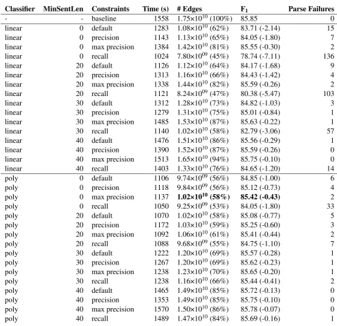
We experimented with a post-processing step to adjust the recall and precision of the classifier, as well as adding a threshold on the minimum length of a sentence to apply constraints to in the parser (on the hypothesis that longer sentences are likely to gain a proportionally larger advantage). We show the detailed results from the parser in Table 8, using both the linear and polynomial classifiers. Sentences shorter thanMinSentLenwere parsed without constraints.

The results are largely as expected. Sentences less than 20 words do not affect the results much. The recall threshold predictably results in a large loss in classifier precision and thus parsing accuracy. We note the results in boldface: with a high precision threshold, the polynomial classifier is able to reduce the computation in the CKY loop by 42% while losing less than half a point in F1

(10)

Classifier MinSentLen Constraints Time (s) # Edges F1 Parse Failures

- - baseline 1558 1.75×1010_{(100%) 85.85} ₀

linear 0 default 1283 1.08×1010_(62%) _{83.71 (-2.14)} ₁₅

linear 0 precision 1143 1.13×1010_(65%) _{84.05 (-1.80)} ₇

linear 0 max precision 1384 1.42×1010_(81%) _{85.55 (-0.30)} ₂

linear 0 recall 1024 7.80×1009_(45%) _{78.74 (-7.11)} ₁₃₆

linear 20 default 1126 1.12×1010_(64%) _{84.17 (-1.68)} ₉

linear 20 precision 1313 1.16×1010_(66%) _{84.43 (-1.42)} ₄

linear 20 max precision 1338 1.44×1010_(82%) _{85.59 (-0.26)} ₂

linear 20 recall 1121 8.24×1009_(47%) _{80.38 (-5.47)} ₁₀₃

linear 30 default 1312 1.28×1010_(73%) _{84.82 (-1.03)} ₃