Public Health Expenditures, Income and Health Outcomes in the Philippines

Public Health Expenditures, Income and

Health Outcomes in the Philippines

Deluna, Roperto Jr and Peralta, Tiffany Faith

University of Southeastern Philippines, School of Applied Economics

April 2014

Online at

https://mpra.ub.uni-muenchen.de/60115/

Tiffany Faye S. Peralta and Roperto S. Deluna, Jr.

Abstract

This paper studied the relationship among public health expenditures, income and health outcomes in the Philippines. Infant mortality rate, under five mortality rate and life expectancy were used as proxy for health outcomes. Specifically, this paper presented the profile of government health expenditures, income and health outcomes from 1981 to 2010. The study used Vector Autoregressive Analysis and Granger Causality test to determine the direction of relationship of the variables.

Results revealed that health expenditure per capita followed an overall increasing trend with an average growth rate of 6.49% and GDP per capita with an average growth rate of 11% from 1981 to 2010. These correspond to the reduction of infant mortality rate by 1.64% on average, under five mortality by 1.76% and the increase in life expectancy with an average growth of 0.17% from 1981 to 2010. However, VAR results revealed that the past values of public health expenditure has no effect on under-five mortality rates but affects infant mortality rate. This may suggest that the past and present level of health expenditure is not sufficient enough to affect under five mortality rate but is effective enough on alleviating infant mortality rate. Conversely, past and present values of GDP per capita is not sufficient enough to affect infant mortality rate but affects under five mortality rate in the Philippines. VAR estimation also revealed that both health expenditure and GDP per capita has a positive and significant effect on life expectancy. Thus, to improve life expectancy and to reduce child mortality rates in line with the Millennium Development Goals, it requires effective and sufficient health expenditure and a sustainable economic growth.

Introduction

It is well-recognized that the government is taking responsibility for the quality of the water that people drink, the level of immunization of a population and campaigns to

stop the spread of HIV/AIDS or to encourage physical exercise. Government-funded public

health activity plays an important part in a country’s health development, through

strengthening health systems and generation of human, financial and other resources. This allows health systems to achieve their goals of improving health, reducing health inequalities, securing equity in health care financing and responding to population needs.

Public expenditure for health care is important for improving health outcomes especially for the poor as the poor are more likely to obtain health care from publicly provided facilities.

Health is indeed closely intertwined with economic growth and sustainable development. There is evidence that investing in health brings substantial benefits for the economy. According to the WHO (2001) increasing life expectancy at birth by 10% will increase the economic growth rate by 0.35% a year. Health and economic matters are intimately linked

in a number of ways. First, health is an important contributor to people’s ability to be

productive and to accumulate the knowledge and skills they need to be productive. Second,

health status is also a major determinant of one’s enrollment in and success in school,

which itself is an important contributor to future earnings. Third, the costs of health care are also extremely important to individuals, especially to poor people, because large out of pocket expenditures can have a major impact on their financial status and can push them to poverty. Fourth, the costs of health care are also very important to countries, because health is a major item of national expenditure of all countries. Finally, the approach that different countries take to the financing and carrying out of health services raises important issues of equity (Jones and Bartlett, 2006).

WHO defines health as a state of complete physical, mental and social well-being and not merely the absence of disease or infirmity. It moves beyond a focus on individual behavior towards a wide range of social and environmental interventions. Another major initiative for improved global health is the United Nations Millennium Declaration. It was agreed to in 2000 by 189 countries including Philippines, exemplifying an unprecedented commitment on the part of both rich and poor countries to attain improvements in human development by the year 2015. This commitment is summarized in the eight Millennium Development Goals (MDGs) that set targets in areas of poverty reduction, health improvements, education attainment, gender equality, environmental sustainability, and fostering global partnerships (UNDP 2003). These movements are formed for the betterment of health outcomes.

Income has a strong effect on health. It imparts more than 75% of total expenditures for health. Past studies show that the poor are significantly less healthy than the rich and that the rich are more likely to obtain medical care. Hence, it is the level of health care financing that can bridge the gap between the health status of the poor and the rich. This indicates that income, as such, is of great importance for the risk of illness (Gwatkin, 2000).

Philippine Context

Life expectancy is also employed as proxy for health outcomes, the intuition is that the longer an average person lives, or the more he spends on health care, the better his health must be. Health outcome is a change in the health of an individual, group of people or

population which is attributable to an intervention or series of interventions (Berkman, et

al, 2011).

In 2010, the government’s main goal in its new health sector plan was to achieve universal

health care under Republic Act No. 7875. The plan was to increase the number of poor people enrolled in PhilHealth, a government mandatory health insurance program that seeks to provide universal health insurance coverage and ensure affordable, acceptable, available, accessible, and quality health care services for all Filipinos, and to improve the outpatient and inpatient benefits package. A full government subsidy is offered to the poorest 20% of the population, and premiums for the second poorest 20% will be paid in partnership with the Local Government Units. This measure has led to an explosion of members and beneficiaries of this component.

Figure 1 shows the public health expenditures among the ten selected Asian countries. Health expenditure of a country should be at least 5% of its Gross Domestic Product (GDP). Based on the 2013 statistics of the WHO, the total health expenditure ratio of the Philippines improved from 3.2% in 2000 to 4.1% in 2010, albeit still below the bench mark.

Philippines ranked 5th _{both in 2000 and 2010. Health spending in the country grew by}

P38.8 Billion or 13.9% annually (www.senate.gov.ph).

Figure 1. Health expenditure as % of GDP, 2000 and 2010. Source: WHO World Health Statistics 2013

In achieving MDG 4 by 2015, reducing child mortality rates, the country set effective and well-defined child health and related programs carried out by the Department of Health, in collaboration with the local government units. The programs offer a range of interventions

0 1 2 3 4 5 6 7 8

HE

as

%

o

f G

DP

that are appropriate at various life cycle stages, from maternal care to care of the newborn up to integrated management of child health.

The economy of the Philippines is one of the emerging markets in the world. However, major problems remain, mainly having to do with alleviating the wide income and growth disparities between the country's different regions and socioeconomic classes and other necessities to ensure future growth.

Figure 2 shows the GDP per capita growth among the ten selected Asian countries, showing the improvement from 2000 to 2010. Income, expressed as GDP per capita has been

significantly improving. The Philippines’ per capita income in 2011 finally stood at about

more than $2,000. Still, it ranked lower among Southeast Asian countries specifically Indonesia with the average of $3,000, $4,700 for Thailand, and $8,400 for Malaysia (IMF, 2013).

Figure 2: GDP per capita growth (annual %), 2000 and 2010

Source: World Bank National Accounts Data

Along with these improved GDP per capita and expenditures for health of the country are observed health outcomes. Over the years, the overall health condition of Filipinos has shown improvement as indicated by declining mortality rates and longer life span. Recent data shows that life expectancy at birth increased by four years over the period 1997-2006, from 67 years in 1997 to 71 years in 2006. Infant and under-five mortality rates have also improved over the years. From 29 infant deaths per 1,000 live births in 2003, the IMR in 2008 improved to 24 deaths per 1,000 live births in 2008. Under-five mortality rate also declined from 40 deaths per 1,000 live births in 2003 to 34 deaths in 2008 (Cabral, 2010).

Objectives of the Study

The general objective of the study is to test the relationship of health expenditures, income and health outcomes in the Philippines. Specifically, the study aims:

1. to present the trend for health expenditures, per capita income and health outcomes

of the Philippines from 1981 to 2010; and

2. to provide empirical evidence on the relationship of health expenditures, GDP per

capita and health outcomes in the Philippines.

0 2 4 6 8 10 12 14

G

DP

p

er

ca

p

it

a

as

%

g

ro

w

th

Conceptual Framework

Several conclusions can be drawn from literatures on the relationship among income, health expenditure and health outcomes. GDP per capita is often considered an indicator of

a country's standard of living or income (Gutierez et al, 2007). Income of households is the

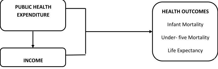
main source on expenditures for health. Health expenditure is invested to improve health outcomes. To the extent that health expenditure increases health outcomes, it will also affect income if healthier populations also produce higher levels of income. As a concept of human capital, health outcomes can also bring improvement to income and can also change the government spending for health. Figure 3 shows the possible flow of relationship between income and health expenditure to health outcomes. Hypothetically, income and health expenditure affects the health outcomes of the country. This effect may either be negative or positive. If positive, this implies that if income and health expenditure increases, it will lead to an improvement on health outcomes of the Philippines. On the other hand if income and health expenditure are found to be insignificant then it implies that income and health expenditure has nothing to do with health outcomes.

Figure 3: Mechanisms relating income and health expenditures on health

outcomes.

Data

The study used annual data of income, health expenditures and health outcomes from 1980 to 2010, a total of 30 observations. Data on health expenditures were obtained from General Appropriations Act (GAA), publication of Department of Budget and Management (DBM). Data on health outcomes and income were obtained from World Bank website.

Statistical Method

The statistical model being done was composed of two phases. Phase I is the analysis of trends of GDP per capita, health expenditure and the 3 health outcomes. Phase II is composed of time series analysis in order to determine the relationships of the aforementioned variables.

PUBLIC HEALTH

EXPENDITURE HEALTH OUTCOMES

Infant Mortality

Under- five Mortality

Life Expectancy

Phase I. Trends of Income, Health Expenditure and Health Outcomes

The trends of income, health expenditure and health outcomes of the Philippines during the period 1981 to 2011 is presented and examined through graphs and tables. The process used Microsoft Excel 2007.

Phase II. Relationship of Income, Health Expenditure and Health Outcomes

Time series analysis was used to identify the relationship of income, health expenditure and health outcomes. A time series is a collection of observations of well-defined data items obtained through repeated measurements over time.

A. Testing for Stationarity

Most time series analysis need to check for unit roots in each series before estimating any equation. According to Granger and Newbold (1974), if there is a unit root then that particular series is considered as non-stationary. The result is stationary if the stochastic

properties of the series remain unchanged over time. ). A stochastic time series {Yt} is said

to be stationary, if and only if, it satisfies the following assumptions:

(1)E[Yt]= µ

(2)Var (Yt)= σ2

(3)Cov (Yt,Yt-k)=σk

Conditions (1) and (2) imply that Yt has a constant means and variance overtime, while

condition (3) means that the covariance between observations depends only on how far apart they are, and not on the time of occurrence (Danao, 2002). If one or more of the above conditions would not be satisfied, it means that the series is non-stationary, and proceeding with regression analysis would result to spurious results, which can produce

high R2 _{and t-statistics, but without any coherent economic meaning or has insignificant}

result.

B. Testing for Unit Roots

Many time series data exhibit trending behavior or nonstationary. If the data are trending, then some form of trend removal is required (Danao, 2002).

To determine whether the data is stationary or not, it is necessary to conduct a standard unit root test. The Augmented Dicky-Fuller (ADF) was used in testing for the presence of unit root and this was applied to the natural logs of the data series (economics.about.com). The time series data in this study could take any of the stationarity models as:

∆Yt = ץY t-1 + εt (random walk) (1)

∆Y t = σ 0 + σ 2 + ץY t-1 + εt (mixed process) (3)

The error term is assumed to be independent and identically distributed. Dickey and Fuller (1981) proposed the ADF test in order to handle the autoregressive process in the variables (Dickey and Fuller, 1979). If the ADF will indicate the occurrence of a unit root, then the series is non-stationary. In case of non-stationary, then we proceed to differencing until we arrive at a stationary series.

Aside from Dickey-Fuller test, Perron test is also used for unit root test. Phillips-Perron test makes a non-parametric correction to the t-test statistic. The test is robust with respect to unspecified autocorrelation and heteroscedasticity in the disturbance process of the test equation.

C. Differencing

Differencing is frequently employed to detrend the data and control autocorrelation by subtracting each datum in a series from its predecessor (www.stat.ucla.edu). In case

stationarity is attained after differencing d times then the series is said to be integrated of

order d (Danao, 2002). In such case, one can then proceed with cointegration analysis. In

this study, the data series were found to be stationary so that the next appropriate analysis is VAR.

D. Lag Order Determination

In order to have an appropriate set of variables to be included in the VAR model, it is necessary to determine the appropriate lag order (Danao, 2002). The popular methods used for lag order determination are the Akaike Information Criterion (AIC), and Schwarz-Bayesian Criterion (SBC). The main idea of AIC is to select the model that minimizes the negative likelihood penalized by the number of parameters. On other hand, Schwarz Bayesian Criterion (Cavanaugh and Neath, 1999) is one of the widely used information criteria. SBC is derived within a Bayesian framework as an estimate to the Bayes factor for two competing models.

Both AIC and SBC differ in their exact definition of a good model. In this case, we will choose the model which has the lowest AIC and SBC value. The AIC and SBC equations are given below:

AIC = Tlog |∑ | + 2N (4)

SBC = Tlog |∑ | + Nlog (T) (5)

Where:

|∑ | = the determinants of the variance /covariance matrix of the residuals;

E. Vector Autoregressive (VAR) Model

According to Sims (1980) and Litterman (1976, 1986) Vector Autoregressive (VAR) models have been proven to forecast better than any simultaneous equation models. Vector

Autoregressive (VAR) models provides information about a variable’s forecasting ability

for the other variable. It is an econometric model used to capture the evolution and the interdependence between multiple time series. A VAR model describes the evolution of a

set of k variables over the same sample period (t=1..., T) as a linear function of only their

past evolution. The variables are collected in a K x 1 vector Yt (or Xt), which has the element

Yt (or Xt), the time t observation of variable Y(or X). A (reduced) p-th order VAR denoted

VAR (p) where the K-periods back observation Yt-k (or Xt-k) is called the K-th lag of Y (or X).

For example, if the Y variable is GDPpc, then Yt is the value of GDPpc at time t

(http://en.wikipedia.org).

In its simplest term, a VAR is an unrestricted form model that expresses each other variable in the system. Using the three variables considered in the study, VAR model specification of a multivariate VAR model is illustrated as:

E.1. Infant Mortality Rate

HExpt C1 A1,1(1) A1,2(1) A1,3(1) HExpt-1 A1,1(k) A1,2(k) A1,3(k) Hexpt-k ε1t

GDPpct = C2 A2,1(1) A2,2(1) A2,3(1) GDPpct-1 +…. A2,1(k) A2,2(k) A2,3(k) + GDPpct-k + ε2t

IMRt C3 A3,1(1) A3,2(1) A3,3(1) IMRt-1 A3,1(k) A3,2(k) A3,3(k) IMRt-k ε3t

E.2. Under five mortality rate

HExpt C1 A1,1(1) A1,2(1) A1,3(1) HExpt-1 A1,1(k) A1,2(k) A1,3(k) Hexpt-k ε1t

GDPpct = C2 A2,1(1) A2,2(1) A2,3(1) GDPpct-1 +…. A2,1(k) A2,2(k) A2,3(k) + GDPpct-k + ε2t

U5MRt C3 A3,1(1) A3,2(1) A3,3(1) U5MRt-1 A3,1(k) A3,2(k) A3,3(k) U5MRt-k ε3t

E.3. Life Expectancy

HExpt C1 A1,1(1) A1,2(1) A1,3(1) HExpt-1 A1,1(k) A1,2(k) A1,3(k) Hexpt-k ε1t

GDPpct = C2 A2,1(1) A2,2(1) A2,3(1) GDPpct-1 +…. A2,1(k) A2,2(k) A2,3(k) + GDPpct-k + ε2t

LEt C3 A3,1(1) A3,2(1) A3,3(1) LEt-1 A3,1(k) A3,2(k) A3,3(k) LEt-k ε3t

where:

t = time subscript;

Hexppct = health expenditure per capita observed at time t;

GDPpct = GDP per capita observed over at time t;

U5MR = under five mortality rate observed at time t;

LE = life expectancy observed at time t;

aij = coefficients of the matrices associated to the VAR, the subscripts

denote the order of the matrix; c1, c2 and c3 = constants; and

ɛt = the error terms

The significant characteristics that the error term must hold in a standard VAR model are as follows:

1. E (ɛt) = 0, where every error term has mean zero;

2. E (ɛt, ɛ’t-k) = Ω, the contemporaneous covariance matrix of error terms is Ω (a

n × npositive definite matrix);

3. E =(ɛt,ɛ’t-k) = 0, for any non-zero k - there is no correlation across time; in

particular, no serial correlation in individual error terms

F. Granger Causality Test

Granger causality takes into account prediction rather than causation as it name would suggest. This is because, in Granger sense, causality is a concept regarding statistical preference and does not necessarily refer to a causal relationship in the economic sense. The approach is based on the idea that the past can cause the future, but the future cannot

cause the past. It is more on “X causes Y”, if the past values of X can be used to predict Y,

better than the past values itself (www.eviews.com). Granger causality can be tested by

using a standard F-test on the lagged values of X, together with lagged values of Y. If results

will generate statistically significant values of X to the explanation of the future values of Y,

this would mean that X Granger causes Y.

Estimation Procedure

The Shazam version 11 was used to test the presence of unit root in the series of variables. To estimate the VAR model and to execute the Granger Causality analysis, the Eviews package version 5 was used.

Results and Discussion

This section shows the time series plots for the health expenditure per capita, GDP per capita and the three health outcomes: infant mortality rate, under five mortality rate and life expectancy of the Philippines from 1981-2010. The trends of the variables for 30 years are all plotted in Figures 3 and 4.

manage secondary level facilities, such as the district hospitals, while the municipalities take charge of the primary level facilities. In 1997, PhilHealth assumed the responsibility of administering the Medicare Programme for government employees from the Government Service Insurance System (GSIS) and in 1998, for private sector employees from the Social Security System (SSS).

Figure 3. GDP per capita, Health Expenditure, Infant and Under Five Mortality of

the Philippines, 1981 to 2010.

There was also an observed increase in health expenditure on 2008 due to the increase in government spending to finance 94% DOH hospitals and also to finance other DOH projects such as Universally Accessible Cheaper and Quality Medicines, Health Sector Development Program, Rural Water Supply and Sanitation Project Phase V, and LGU Urban Water and Sanitation Project. The government had incurred additional loans to fund the said projects. It is also observed that there was a large increase of health expenditure in 2009 which accounts 40% increment from the previous year . According to the WHO, the ideal health expenditure of developing countries must be 5% of the GDP of the country.

However, Philippines’ health expenditure has only about 4.1% of GDP as of 2010

(en.wikipedia.org).

The GDP per capita series used as proxy for income in this study that is presented in Figure 3. It follows a smooth increasing trend from 1981 to 2010 with an average growth rate of 11%, an indication of nonstationary process. Despite of the increasing trend, it is noticeable that GDP per capita decreased from 1984 to 1985 which accounts a -7.31% growth rate. During these years, economic misconduct and political instability during the Marcos regime contributed to economic stagnation and resulted in macroeconomic instability. There was a severe recession from 1984 through 1985. The real GDP of the country continued to increase in the subsequent years. In 2008, Philippines was in its difficult year the growth slowed significantly and poverty increased, driven in part by rising fuel and food prices.

0 10 20 30 40 50 60 70 80 90 0 50 100 150 200 250 300 350 19 81 19 82 19 83 19 84 19 85 19 86 19 87 19 88 19 89 19 90 19 91 19 92 19 93 19 94 19 95 19 96 19 97 19 98 19 99 20 00 20 01 20 02 20 03 20 04 20 05 20 06 20 07 20 08 20 09 20 10 In fant an d Und e r Fi v e M o rtlai ty R ate (% ) H e al th E xp e n d itu e (i n p e sos), GDP p e r cap ita (i n t h o u san d p e sos)

However the real gross domestic product recovered from stagnation and achieved a better performance in proceeding years. Furthermore, the real Gross Domestic Product (GDP) has been on an upward trend until 2010.

These increasing level of health expenditure and GDP per capita are accompanied by a reduction of infant mortality rate by 1.64% and under five mortality rate by 1.76% from 1981 to 2010. This reduction means an improvement on the status of mortality rates. Figure 3 shows an overall decreasing trend especially from 1981 to 2006. Infant mortality rate is continuously decreasing from 51.4% in 1981 to 21% in 2010. Under five mortality rate shows a more decreasing trend compared to infant mortality rate, which declines from 76.9% in 1981 to 26.4% in 2010. The target of MDG for 2015 is to reduce infant mortality rate to 19% and 26.7% for under five mortality rate. The figure shows that the country has high possibility on achieving these goals.

Life expectancy, another indicator for health outcomes have shown continuous increasing trend from 1981 to 2010 with an average of 0.167 as shown in figure 4. Life expectancy has improved from 63.7 in 1981 to 68.5 in 2010.

Figure 4. GDP per capita, Health Expenditure and Life Expectancy in the Philippines, 1981

to 2010.

Generally, Figures 3 and 4 shows improvement of health outcomes along with increasing levels of GDP per capita and health expenditures. To empirically examine the relationship among these variables, Vector Autoregressive Analysis was employed.

60 61 62 63 64 65 66 67 68 69 0 50 100 150 200 250 300 350

1981 1982 1983 1984 1985 1986 1987 1988 1989 1990 1991 1992 1993 1994 1995 1996 1997 1998 1999 2000 2001 2002 2003 2004 2005 2006 2007 2008 2009 2010

Li fe E xp e catan cy ( n u m b e r o f y e ar s) H e al th E xp e n d itu re (i n p e sos), GD P p er cap ita ( in t h ou sa n d p esos)

Relationship among Income, Health Expenditure and Health Outcomes

Stationarity Tests

In dealing with time series analysis, the stationarity properties of the series are important. This was initially tested using correlograms derived from Autocorrelation Function (ACFs) and Partial Autoccorelation Functions (PACFs).

The correlograms of the ACF and PACF of Hexp, GDPpc, IMR, U5MR, and LE are presented in Appendices 1 to 3 respectively. The results show that the correlograms of the aforementioned variables are decaying rapidly which is an indication of a stationary series. However, due to the possibility of subjective conclusions that can be derived from evaluating stationarity through graphs, Augment Dickey-Fuller tests were performed to check formally if the series are statistically stationary. Results of the unit root tests are summarized in Table 2.

Table 2. Augmented Dickey Fuller (ADF) test results.

Variable Random Walk Random Walk w/

Drift

Mixed Process

Hexppc GDPpc

IMR U5MR

LE

1.4075ns

15.173* -3.9478* -3.7944* -27.587*

0.21938ns

8.4320* -4.2125* -3.7131* -7.1449*

1.5122ns

36.843* 9.0176* 6.7228*

39.592*

ns not significant at 10% level * Significant at 10% level

The test results for presence of unit roots for the aforementioned variables revealed that the series are stationary confirming earlier results from the correlogram except for health expenditure per capita. The values are tested at 10% significant level.

Differencing of Health Expenditure per capita

The result of the ADF test revealed that series of Hexppc exhibits unit root. This would

mean that Hexppc is nonstationary. The main premise for differencing health expenditure

per capita is to remove the underlying trend effect. Using the first difference value (Appendix 5), the variable was found to be stationary at first differencing. This implies that the variable attained stationarity after first differencing and the series is said to be

integrated of order 1.

Table 3 presents the result of the ADF test for the variable Hexppc after first differencing.

Table 3: Augmented Dickey Fuller (ADF) test results for Hexppc in first differenced.

Variable Random Walk Random Walk with Drift Mixed Process

Hexppc -3.9666* -4.2421* -4.3157*

This is significant under the three processes.

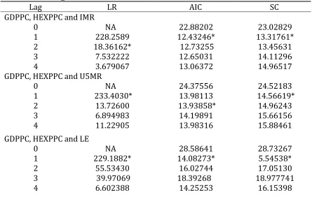
Lag Order Determination

Cointegration is not possible in this study since the variables are not integrated of the same order, the next alternative estimation would be the Vector Autoregressive (VAR) modeling. Specification of correct lag order in VAR modeling is one of the important components to

be considered in time series analysis. The selection of inappropriate p will decrease the

accuracy of the estimated coefficients in VAR (p) model. In determining the lag, the lowest

value of AIC and SBC was the chosen lag of the variables. In addition, the highest value of LR test statistic also helps in determining the lag order. VAR lag order selection were done

using EViews package version 5.0. Table 4 shows the results of lag order selection of the

three VAR models.

Table 4: VAR Lag Order Selection Criteria.

Lag LR AIC SC

GDPPC, HEXPPC and IMR

0 NA 22.88202 23.02829

1 228.2589 12.43246* 13.31761*

2 18.36162* 12.73255 13.45631

3 7.532222 12.65031 14.11296

4 3.679067 13.06372 14.96517

GDPPC, HEXPPC and U5MR

0 NA 24.37556 24.52183

1 233.4030* 13.98113 14.56619*

2 13.72600 13.93858* 14.96243

3 6.894983 14.19891 15.66156

4 11.22905 13.98316 15.88461

GDPPC, HEXPPC and LE

0 NA 28.58641 28.73267

1 229.1882* 14.08273* 5.54538*

2 55.53430 16.02744 17.05130

3 39.97069 18.39268 18.977741

4 6.602388 14.25253 16.15398

* indicates lag order selected by the criterion

LR: sequential modified LR test statistic (each test at 5% level) AIC: Akaike information criterion

SC: Schwarz information criterion

Vector Autoregression (VAR) Analysis

A VAR is a simultaneous system of equations that examine the economic inter-relationship

of variables which provides a statistical representation of the variables’ past interactions.

Within this framework, all variables are treated symmetrically without any distinction of which variable is exogenous and endogenous. The variables were tested at 10% significant level. Table 5, 6 and 7 shows the VAR estimation results and the standard errors of the three VAR models.

a. Infant Mortality Rate

Table 5 shows the result of the VAR estimation outputs and the standard error of the VAR models consisting Hexppc, GDPpc, and IMR with a lag length of 1. Results revealed that

infant mortality rate is reduced by an increased in the previous year’s health expenditure.

That is, a thousand peso increase in health expenditure in the previous year will statistically reduce the current infant mortality rate by a very minimal 0.000025%.

Table 5. Estimates for the Unrestricted VAR (1) Model for the Health Expenditure, GDP per capita and Infant Mortality Rate.

GDPPC HEXPPC IMR

HEXPPC(-1) 0.079435ns _3.054915ns _-0.000025*

(0.21170) (2.71343) (0.0000068)

GDPPC(-1) 0.004588ns _{0.886873* -0.000000101}ns

(0.00620) (0.07946) (0.0000002)

IMR(-1) 33.04187ns _{3561.649* 1.024613*}

(83.2308) (1066.79) (0.00268)

C -57.39521ns _228.6579ns _0.003668*

(61.5164) (788.470) (0.00198)

Adj. R-squared 0.1119268 0.926638 0.999887

Log likelihood -132.0612 -203.4834 157.5102

Akaike AIC 9.718658 14.82024 -10.96502

Schwarz SC 9.908973 15.01055 -10.77470

Log likelihood -177.3056

Akaike information criterion 13.52183

Schwarz criterion 14.09277

*Significant at 10% level ns_{Not significant at 10% level}

year’s values of GDP per capita and infant mortality rate. However, GDP per capita or improvement in income in the previous year has no effect on current level of infant mortality rate. This might suggest that GDP per capita is not sufficient to affect infant mortality rate.

b. Under Five Mortality Rate

Table 6 shows the result of the VAR estimation outputs and the standard error of the variables, HEXPpc, GDPpc, and U5MR with a lag length of 1. Results showed that health expenditure is not sufficient enough to affect under five mortality rate. However, results revealed that the value of GDP per capita a year ago improves the level of under-five

mortality rate at the current year. Also, an improvement on last year’s level of under-five

mortality rate will bring substantial progress to its level at present.

Table 6. Estimates for the Unrestricted VAR (1) Model for the Health Expenditure,

GDP per capita and Under Five Mortality Rate.

GDPPC HEXPPC U5MR

HEXPPC(-1) 0.081771ns _3.331539ns _-0.0000179ns

(0.21215) (2.76184) (0.000017)

GDPPC(-1) 0.005515ns _0.939606ns _-0.00000158*

(0.00562) (0.07319) (0.00000044)

U5MR(-1) -8.711931ns _-1727.060ns _0.980688*

(42.1492) (548.719) (0.00329)

C -53.03020ns _1658.092ns _-0.026718*

(78.6466) (1023.86) (0.00614)

Adj. R-squared 0.224138 0.923954 0.999763

Log likelihood -132.1279 -203.9863 132.6711

Akaike AIC 9.723425 14.85617 -9.190795

Schwarz SC 9.913740 15.04648 -9.000480

Log likelihood -199.2623

Akaike information criterion 15.09017

Schwarz criterion 15.66111

*Significant at 10% level ns_{Not significant at 10% level}

c. Life Expectancy

revealed that the value of health expenditure and GDP per capita a year ago has a positive effect to life expectancy. Thus, this implies that an increased health expenditure and GDP per capita a year ago would lead to an improvement in life expectancy at present.

Table 7. Estimates for the Unrestricted VAR (1) Model for the Health

Expenditure, GDP per capita and Life Expectancy.

GDPPC HEXPPC LE

HEXPPC(-1) 0.080689ns _{3.140121 0.000498*}

(0.21211) (2.77861) (0.00011)

GDPPC(-1) 0.005394ns _{0.933898* 0.0000106*}

(0.00570) (0.07470) (0.000003)

LE(-1) 1.139634ns _{193.4058* 0.982426*}

(4.78862) (62.7304) (0.00253)

C -130.9375ns _{-11865.94* 1.197472*}

(289.023) (3786.17) (0.15250)

Adj. R-squared 0.323546 0.923045 0.999870

F-statistic 0.792965 108.9512 69149.22

Log likelihood -132.1198 -204.1528 79.19857

Akaike AIC 9.722846 14.86806 -5.371326

Schwarz SC 9.913161 15.05837 -5.181011

Log likelihood -253.1702

Akaike information criterion 18.94073

Schwarz criterion 19.51167

*Significant at 10% level ns_{Not significant at 10% level}

Granger Causality Test

The three VAR models test about the relationship among health expenditure per capita and GDP per capita of the three different health outcomes are limited to the current and lag values of the variables. The Granger Causality test will further determine if the historical values of one variable can forecast relationships among other variables. This test was done on the three models. Table 8 presents the Granger causality test of variables. The null hypotheses were subjected to F-test at 10% significant level.

lead to improved income and an increase in real GDP per capita. Results revealed that the three health outcomes can forecast the future values of GDP per capita.

Table 8. Results of the Granger Causality Test

Null Hypothesis: F-Statistic Probability

GDPPC does not Granger Cause HEXPPC 1.50276 0.23167ns

HEXPPC does not Granger Cause GDPPC 1.03808 0.31803ns

IMR does not Granger Cause HEXPPC 1.08160 0.30830ns

HEXPPC does not Granger Cause IMR 13.5383 0.00112*

IMR does not Granger Cause GDPPC 10.8024 0.00290*

GDPPC does not Granger Cause IMR 5.17847 0.03135*

U5MR does not Granger Cause HEXPPC 0.52621 0.47494ns

HEXPPC does not Granger Cause U5MR 0.02977 0.86440ns

U5MR does not Granger Cause GDPPC 9.44156 0.00493*

GDPPC does not Granger Cause U5MR 12.3859 0.00161*

LE does not Granger Cause HEXPPC 0.61060 0.44190ns

HEXPPC does not Granger Cause LE 24.7918 0.000039*

LE does not Granger Cause GDPPC 8.94487 0.00602*

GDPPC does not Granger Cause LE 23.6805 0.000048*

*Significant at 10% level ns_{Not significant at 10% level}

Summary and Conclusion

Results of trends analysis revealed that GDP per capita, with an average growth rate of 11%, is continuously increasing through the period 1981 to 2010. Health expenditure, with an average growth rate of 6.49%, has shown fluctuating trend in early years but shows a distinctive increase in the later part. These correspond to the reduction of infant mortality rate by 1.64% on average, under five mortality rate by 1.76% and the increase in life expectancy with an average growth rate of 0.17% from 1981 to 2010.

expenditure for health outcomes is being implemented by the government, little empirical evidence exists on the beneficial impact of such expenditure to child mortality rates.

The results also revealed that GDP per capita affects the under-five mortality rate but is not sufficient enough to affect infant mortality rate in the Philippines. This implies that an

increase in the past year’s values of GDP per capita would lead to a reduction of under- five

mortality rate at the current year. On the other hand, both public health expenditure and

GDP per capita has a positive effect to life expectancy. Thus, the previous year’s increased

value of health expenditure and GDP per capita increases the level of life expectancy at present.

Results on Granger causality test revealed that GDP per capita does not forecast the future values of health expenditure, and vice versa. Results also suggest that health expenditure can predict future levels of infant mortality rate and life expectancy, but not vice versa. Furthermore, it suggests that health outcomes can be predicted by GDP per capita and vice versa.

From these results, the study makes the following conclusions: First, even joint efforts were made on the improvement of GDP per capita, it is not sufficient enough to affect infant mortality rate possibly because GDP per capita, used to proxy income in this study, is not used to spend and focus to health care alone. Second, expenditures for reducing infant deaths have been addressed by the programs and projects implemented by the government, but, an increasing expenditure for health still has no effect to under five mortality rate. This may suggest that the level of public health expenditure is not sufficient enough to have significant improvements on the reduction of under-five mortality rate.

RECOMMENDATIONS

Based from the results and conclusion, the following recommendations are made:

Public health expenditure has a statistically significant effect to infant mortality rate and life expectancy. From the ever increasing public health expenditure, the government must improve policies concerning the three health outcomes and the expenditures should be rightfully evaluated. Improvements in health expenditure will be a big assistance in order

to reach the 4th _{goal of the Millennium Development Goal on reducing child mortality.}

It is proven in this study that GDP per capita brings an improvement to under five mortality rate and life expectancy but not to infant mortality rate. All efforts should be exerted to sustain economic growth in the country and these efforts will then lead to a further improvement of health outcomes.

References:

Anyanwu, J. and A. E. Erhijakpor (2007). Health Expenditures and Health Outcomes in

Africa. Delta State University Economic Research Working Paper No. 91.

Bloom, D., D. Canning, J. Sevilla (2004). The Effect of Health on Economic Growth: A

Production Function Approach. Harvard School of Public Health, Boston, MA, USA. World Development Vol. 32, No. 1, pp. 1–13, 2004.

Bokhari, F., Y. Gai, P. Gottret (2006). Government Health Expenditures and Health

Outcomes. Department of Economics, Florida State University.

Berkman, N., S Sheridan, K. Donahue, D. Halpern, K. Crotty (2011). Low health

literacy and health outcomes: an updated systematic review. Research Triangle Park, North Carolina 27709-2194, USA. berkman@rti.org

Bryant, J. (2004). Population Ageing and Government Health Expenditures in New Zealand,

1951-2051

Cabral, E. (2010). Statement at 43rd Session of the Commission on Population and

Development.

Day, K. and J. Tousignant (2005). Health Spending, Health Outcomes, and Per Capita

Income in Canada: A Dynamic Analysis. Department of Economics, University of Ottawa Working Paper 2005-2007 (June).

Fogel, R. (2009). Forecasting the Costs of US Health Care.

Gardner H. and B. Gardner (2001). Health as Human Capital Theory and Implications.

http://connect.msbcollege.edu/bbcswebdav/pid-1637171-dt- content-rid31106_1/library/Graduate/MG565/External%20Link/Week%201% 20Theory.pdf

Gani, A. (2008). Health Care Financing and Health Outcomes in Pacific Island Countries.

Macmillan Brown Centre for Pacific Studies.

Gwatkin, D.R. (2000). Reducing Health Inequalities in Developing Countries. Oxford

Textbook of Public Health fourth edition, 2002

Jones, D and A. Bartlett (2006). Health, Education, Poverty and the Economy.

Kim, T. and S. Lane (2013). Government Health Expenditure and Public Health

Outcomes: A Comparative Study among 17 Countries and Implications for US Health Care Reform Vol. 3 No. 9 (September).

Ogungbenle, S., O.R. Olawumi, F. Obasuyi (2011). Life Expectancy,Public Health

Spending and Economic Growth in Nigeria. Department of Economics, Ikere Ekiti Vol. 9 No. 19.

Qadri, F.S., and Dr. A. Waheed (2011). “Human Capital and Economic Growth:

Time Series Evidence from Pakistan”. MPRA Paper No. 30654.

Solon, O., A. Herrin, R. Racelis. M. Manalo, V. Ganac (1999). Health Care Expenditure

Patterns in the Philippines: Analysis of National Health Accounts, 1991-1997 Vol. 36, No. 2.

Online References:

en.wikipedia.org

siteresources.worldbank.org

www.fes.org.ph

www.economics.about.com www.google.com

www.indexmundi.com www.nscb.gov.ph