Urban traffic state estimation & prediction

(1)

URBAN TRAFFIC STATE

ESTIMATION & PREDICTION

Master Thesis

(2)

2 Title:

Author:

Date:

Contacts:

Urban traffic state estimation & prediction

Luuk de Vries

University of Twente

Civil Engineering & Management Traffic Engineering & Management S1003712

[email protected]

21th_{of October 2016}

Daily Supervisor

Luc Wismans

University of Twente Tel: 0570 - 666 840

Email: [email protected]

UT Supervisor

Eric van Berkum University of Twente Tel: 053 - 489 1098

(3)

3

1

2 Abstract (Dutch)

In de laatste jaren wordt informatietechnologie (IT) in het verkeer steeds vaker toegepast en onderzocht. Het gebruik van IT in zowel voertuigen als infrastructuur, valt onder de noemer van intelligente transportsystemen (ITS). Voordelen van het toepassen van ITS zijn divers en kunnen variëren van; een verhoogde verkeersveiligheid, verbeterde prestaties van het verkeersnetwerk, verbeterde mobiliteit, milieuvoordelen tot economische groei (Ezell, 2010). Typisch gebruik van ITS leunt op een belangrijk ingrediënt; een robuust, volledig en accuraat beeld van de verkeerstoestand in het netwerk. Dit beeld wordt gerealiseerd in een proces welke wordt omschreven als traffic state estimation. Het verlengde van dit proces, de traffic state prediction, voegt daar een extra stap aan toe door de verkeerstoestand in het netwerk te voorspellen voor de (nabije) toekomst.

In dit onderzoek met als onderwerp urbantraffic state estimation- en traffic state prediction, worden twee algemene uitdagingen geïdentificeerd. Als eerste is er een mismatch tussen de hoeveelheid beschikbare meetgegevens en de te schatten en voorspellen verkeersstroomvariabelen. Een verkeersnetwerk wordt immers nooit volledig door verkeersinformatiebronnen gedekt, waardoor technieken nodig zijn om de data die wel beschikbaar is, zo goed mogelijk te extrapoleren en te gebruiken. De tweede uitdaging ontstaat door in dit onderzoek te focussen op een stedelijke omgeving. Een stedelijke omgeving verhoogt de moeilijkheidsgraad, als gevolg van bijvoorbeeld lagere verkeersvolumes, lagere maximumsnelheden, meer variatie in snelheden, een hogere dichtheid van kruispunten, verkeerslichten, rotondes, prioriteiten en dynamische interacties tussen vervoerswijzen, in tegenstelling tot een netwerk dat enkel uit snelwegen bestaat.

Van Hinsbergen et al. (2007) beschrijft dat er reeds een grote hoeveelheid methodes bestaan voor

traffic state estimation en traffic state prediction. Er zijn naïeve modellen, parametrische modellen, niet-parametrische modellen en een hybride mengsel van twee of meer van deze categorieën. Van Lint (2011) benadrukt dat het vinden van een balans tussen geavanceerde en complexe modellen aan de ene kant en robuuste, snelle en algemeen toepasbare modellen aan de andere kant, het grootste probleem in de praktijk van traffic state-estimation en –prediction is.

De naïeve categorie vertegenwoordigt de modellen, waarbij verkeersgegevens alleen gebruikt worden om daaruit directe relaties te berekenen. Voorbeelden zijn instantaneous travel time of

historical averaging modellen. Voordelen van deze modellen zijn de lage berekeningscomplexiteit en eenvoudige implementatie. Het nadeel is dat vanwege het weglaten van de verkeersstroomtheorie, de uitkomsten doorgaans onlogisch of onnauwkeurig zijn. De parametrische categorie

vertegenwoordigt modellen waarin het principe van Lighthill-Whitham-Richards (Lighthill & Whitham, 1955) wordt toegepast. Klassieke voorbeelden zijn; Newell’s simplified kinematic wave model (Newell, 1993) en cell transmission models (Daganzo, 1994). Het voordeel van deze modellen is dat de verkeersstroomtheorie wèl gebruikt wordt, maar met als nadeel dat veel kalibratie van parameters nodig is. Een ander nadeel is dat door de stedelijke omgeving van het netwerk in dit onderzoek, de fundamenten van de verkeersstroomtheorie niet noodzakelijk meer gelden, wat de betrouwbaarheid van deze modellen negatief beïnvloed. De niet-parametrische categorie omvat de modellen waarin relaties uit de verkeersgegevens worden beschouwd, maar geen parameters worden geschat. Voorbeelden van deze modellen zijn meestal gebaseerd op lineaire regressie. Deze modellen hebben gemeen dat ze een lage complexiteit hebben en daardoor gemakkelijk in real-time kunnen worden uitgevoerd. De nauwkeurigheid is volgens Van Lint (2011) echter meestal laag.

Theoretisch meer geschikt voor de stedelijke toepassing zijn hybride model types, welke elementen van niet-parametrische, parametrische en naïeve methoden combineren. Het meest bekende

(7)

7

Het doel van dit onderzoek is om een kader te ontwerpen voor traffic state estimation en traffic state prediction, in een stedelijke omgeving, welk gebruik maakt van zowel floating car- en tellus data om real-time en toekomstige uitspraken te doen over de snelheid, dichtheid en intensiteit op iedere link in het netwerk. Als uitgangspunt voor dit ontwerp worden de methoden van Morita (2011) en Esaway (2012) gebruikt. De nieuw ontworpen Neighbourhood Link Method (NLM) wordt vervolgens beoordeeld op de nauwkeurigheid van de schattingen en voorspellingen.

De gebruikte onderzoeksmethode bestaat uit drie afzonderlijke delen; 1) het simuleren van de z.g.

ground truth, 2) de traffic state estimation en 3) de traffic state prediction. In het eerste deel van het onderzoek wordt een microsimulatie programma (PARAMICS) gebruikt om een 100% accuraat en 100% dekkende ground truth te genereren in het als case gekozen Sioux Falls verkeersnetwerk. Deze

ground truth blijft verder ongewijzigd gedurende dit onderzoek. Het tweede deel van dit onderzoek beschrijft de totstandkoming van de NLM voor traffic state estimation. Dit raamwerk wordt

vervolgens onderworpen aan een evaluatie met als doel om het ontwerp verder te verbeteren. Met de ground truth beschikbaar voor vergelijkingsdoeleinden, worden de schattingen beoordeeld op juistheid. In het derde deel wordt deze procedure herhaalt, om het NLM raamwerk uit te breiden voor traffic state prediction.

Het nieuw ontwikkelde NLM raamwerk, bestaat uit 7 stappen. Aanvankelijk worden gemeten verkeersgegevens ongewijzigd opgeslagen in een database. Vervolgens worden de links welke zich over de tijd hetzelfde gedragen aan elkaar gekoppeld (neighbours/buren) op basis van correlatie. De mest recente real-time beschikbare verkeersdata wordt vervolgens gebruikt om uitsluitend de verkeersdata van de buren, met behulp van lineaire regressie, om te zetten in een z.g. buurt-schatting van verkeersvariabelen voor een wegvak. Deze wordt vervolgens gefuseerd op basis van betrouwbaarheid, met de meest recente verkeersdata van de link zelf om de traffic state estimation

te realiseren. Voor het voorspellen, wordt aan het raamwerk een tijdsdimensie gelijk aan de voorspelhorizon toegevoegd, om met de meest recente verkeersdata de toekomst te voorspellen.

De resultaten laten zien dat NLM bij 5% FCD; gemiddeld 60% van de stedelijke segmenten in het netwerk binnen 5km/uur (3 mi/h) van de waarheid kan schatten, gedurende de spits. Buiten de spits daalt dit percentage tot 50%. De dichtheid wordt voor 80% van de segmenten geschat binnen 7,5 vtg/km/rijstrook en voor de intensiteitsschattingen geldt dat voor 60% van de segmenten binnen 100 vtg/uur/rijstrook kunnen worden geschat. Met bijbehorende correlatie waarden van meer dan 0,91 voor snelheid; 0,93 voor dichtheid en 0,75 voor intensiteit. Het NLM raamwerk voor voorspelling laat bij 5% FCD en een voorspelhorizon van 5 minuten opnieuw veelbelovende resultaten zien, met slechts een 20% reductie in nauwkeurigheid van snelheidsvoorspellingen. Echter de dichtheid is tot 50% minder nauwkeurig, en intensiteitsvoorspellingen zijn zelfs tot 300% slechter. De correlatie van de snelheid en dichtheid voorspellingen daalt slechts marginaal, maar de correlatie van intensiteit daalt met 10% tot 15%. Voor een voorspelhorizon van 15 minuten neemt de zowel de

nauwkeurigheid als de correlatie verder af tot voor de correlatie ver onder de 0,75.

Dit onderzoek laat zien dat het ontworpen NLM raamwerk een veelbelovende traffic state estimation

(8)

8

3 Abstract

The use of information technology (IT) in traffic systems is becoming a hot topic within the traffic research community. It is within this context that IT and traffic, blend together to create intelligent transportation systems (ITS). Benefits of employing ITS are ample and can range from; increased safety, improved operational performance, enhanced mobility, environmental benefits to boosts of productivity leading to economic and employment growth (Ezell, 2010). One of the practical outcomes can for example be that all actors of the transportation systems are allowed to enlighten themselves with information and make better informed decisions. This type of utilization of ITS leans on a key ingredient; a robust, complete and accurate picture of the traffic state in the network. This picture is generated in a process called traffic state estimation. It generally goes hand in hand with the process of traffic state prediction, which produces the future pictures of the traffic state.

In this research towards urban traffic state estimation and prediction, two challenges are introduced. Firstly there is a mismatch between the amount of data and the needed traffic flow variables. A traffic network is in practice never fully covered by traffic information sources, thus requiring

techniques to extrapolate and utilize the traffic data that ís available. The second challenge is a result of choosing an urban environment as subject of study in this research. An urban environment which as opposed to a freeway only network, comes with a higher complexity due to e.g. lower traffic volumes, lower speed limits, more variability in velocities, a higher density of intersections, traffic signals, roundabouts, priority-junctions and dynamic interactions between other modes of transport.

Van Hinsbergen et al. (2007) describes that the vast amount of traffic estimation and predictions models used in literature can be fitted into four categories. There are naïve models, parametric models, non-parametric models and a hybrid blend of two or more of these categories. Van Lint (2011) emphasizes that the key difficulty for traffic state estimation and prediction is therefore to find a balance between sophisticated and complex models on one side and smooth, fast, general applicable models on the other side, to make valid estimations and forecasts given the data available.

The naïve categorization represents models, in which only traffic data is used from which direct relations are calculated. Examples are instantaneous travel time or historical averaging models. The advantage of these models is the favourable low computational complexity and easy to

implementation. The downside is that because of the lack of traffic theory, results are usually illogical and inaccurate. The parametric categorization represents models in which the principle of the Lighthill–Whitham–Richards (Lighthill & Whitham, 1955) model are applied. Classical examples are; Newell’s simplified kinematic wave model (Newell, 1993) and cell transmission models (Daganzo, 1994). The advantage of these models is that they implement logical real world traffic theory, but with the disadvantage of requiring vast calibration of parameters. Additionally due to the case being an urban network where the traffic flow fundamentals of for example flow conservation might not be applicable, accuracy is negatively affected. The non-parametric categorization represents the traffic models in which relations in traffic data are considered, but no traffic flow parameters are estimated. Examples of these models are mostly based on simple regression. These models have in common that while their complexity is low and therefore they can easily be run in real-time speed, their accuracy is according to Van Lint (2011) generally fairly low.

(9)

9

The goal of this research is to design a performing traffic state estimation and traffic state prediction framework, which by utilizing both floating car- and inductive loop detector- data, delivers real-time and future link -velocities, -densities and -flows within an urban traffic environment. Used as a starting point for this design are the previously methods of Morita (2011) and Esaway (2012), from which this newly developed neighbourhood link method (NLM) is created. Aimed is to answer the question on how to design a neighbour link framework which delivers both a traffic state estimation and state prediction of all relevant traffic flow variables within an urban network and assess both the performance and accuracy of the traffic states outputted by this NLM framework.

The research method applied is divided into three separate parts; 1) the urban traffic state ground truth, 2) the urban traffic state estimation and 3) the urban traffic state prediction part. In the first part of the research a microsimulation programme (PARAMICS) is used to generate a 100% accurate and 100% covered ground truth for the Sioux Falls network. This ground truth designed remains unchanged throughout this research. The second part of this research presents the extension of the ground truth framework with the NLM for traffic state estimation. Additionally the steps of

performance assessment, evaluation and synthesis are included to complete the design cycle. With the ground truth available (for comparative purposes), the estimations are assessed on accuracy and correlation leading to the designing of the best performing NLM variant for both traffic

state-estimation and -prediction.

The newly developed NLM framework can be described by the following 7 steps. Initially traffic data is stored in a database. Next from this database for each link it is determined which links behave the same and can be considered neighbours based on correlation in traffic data. Then newly arrived data is considered upon which an estimation from solely the traffic data of neighbouring links is generated using linear regression. Consequently this neighbourhood estimation is fused, weighted on reliability, with the traffic data from the link itself, generating the final traffic state estimation. For the

prediction part, an extra time dimension is included, to incorporate the prediction horizon.

The results reveal that the NLM framework for estimation at 5% FCD, is able to estimate on average 60% of the urban links in the network within 3 mi/h of the ground truth during rush hour periods. In free flow traffic this percentage drops to 50%. Density estimations show 80% of all links to be estimated within 12 veh/mi/lane and of the flow estimations 60% of the links can be estimated within 100 veh/h/lane deviations in rush hour. With corresponding correlation values of over 0,91 for velocity; 0,93 for density and 0,75 for flow estimations. The NLM framework for prediction shows at 5% FCD and a prediction horizon of 5 minutes again promising results, with only a 20% drop in accuracy for velocity. However density predictions are up to 50% less accurate, and flow predictions are up to 300% worse. The correlation of velocity and density predictions only drop marginally, but the correlation of flow predictions lowers by 10% to 15%. For a prediction horizon of 15 minutes the degradation continues as the prediction accuracy decreases further and the correlation for density and flow drops well below 0,75.

(10)

10

4 Introduction

4.1 Preface

Information technology (abbreviated as IT) is currently being applied on a global scale. In education, health, industries and in government the role of IT has become more and more important in the last few years. With the positive effects of IT not going unnoticed, IT use in traffic systems is also on the rise. For many countries, building new roads and other traffic infrastructure to keep up with the ever growing traffic demand, is no longer a viable solution. The scope is turning from asphalt, concrete and steel to more intelligent use of the traffic infrastructure currently in place. It is within this context that IT and traffic blend to the subject of intelligent transportation systems (ITS). ITS gives the actors of the transportation systems (both the controllers as the actual users) the power to enlighten themselves with information (in all kinds of formats) to make better informed decisions. Examples of these decisions are ample on the user side; e.g. route choice behaviour, departure time behaviour and mode choice behaviour, yet also on the controller side; e.g. automatic incident detection (AIDA) (Wang, 2005), optimizing traffic signals, improve current roads and provide better public transportation. ITS can deliver five key benefits; increasing safety, improving operational performance, enhancing mobility and convenience, delivering environmental benefits, and lastly boosting productivity leading to economic and employment growth (Ezell, 2010).

A key ingredient of ITS is real-time traffic information. It is therefore required to somehow get a complete image of the network’s traffic state at current and near future times (Wang, 2005) to derive this traffic information from. The more accurate this image the more focussed ITS can be implemented for actors in the traffic network. The task of mathematically deriving an image of the network’s traffic state from traffic data, are separated into the traffic state estimation- and traffic state prediction task. The goal of both is to deliver a robust, complete and accurate picture of the urban traffic state on all links in the network.

The traffic state estimation task refers in this context to real-time estimation of different traffic flow variables for a network within a specific time interval and spatial resolution. The traffic state

prediction task refers to real-time prediction over a certain time horizon of different traffic flow variables for a network within a specific time interval and spatial resolution. Both the estimation and prediction are generated by applying mathematical techniques and concepts of traffic flow, upon available real-time traffic data.

Within the research field of traffic state estimation and prediction, a recent shift has occurred altering the scope of research from the relative comfort of freeway segments in highway networks to larger and more detailed urban road networks. These urban networks cover besides the upper network also the important primary and secondary urban arterials. A first example of such an urban study is the Instrumented City Project (Bell et al. 1992). Practical examples of recent urban traffic state studies in the Netherlands are Sensor City Assen (as from 2011) and the Praktijkproef

Amsterdam (as from 2013). Within both these projects and in literature, the traffic flow variables of interest are; link wise space mean speeds, travel times, traffic densities and flows (e.g. Snelder & Calvert, 2015; Wang, 2005). Accurately estimating these traffic flow variables for different pre-defined network segments is the ultimate goal for the application of traffic state estimation techniques. Additionally predicting these traffic flow variables is the goal of the traffic prediction counterpart. As the number of unknown traffic flow variables to be estimated and predicted are generally larger than the number of variables that are measured, the relative complex task of a deriving an accurate real-time network traffic state for ITS purposes, becomes visible.

(11)

11

4.2 Problem definition

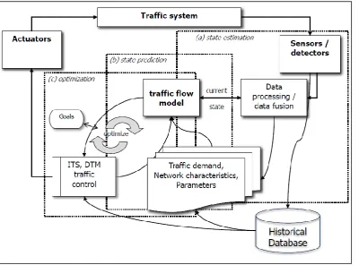
[image:11.595.74.475.313.609.2]

Research into urban traffic state estimation and prediction comes with two challenges. Firstly there is the previously mentioned mismatch between the amounts of big data and the needed traffic flow variables. The urban network is in practice never fully covered by traffic information sources, leading to gaps and errors when no techniques are applied to the traffic data that ís available. The second challenge is related to the urban nature of the traffic network. While research on traffic state estimation on freeways is vast (Nantes, 2015), literature on traffic state estimation in an urban environment is less common. It is however not less interesting, as negative effects of traffic affect a larger population in urban areas than in rural areas. The ante is upped because of the fact that an urban environment provides additional challenges as opposed to a freeway only network, due to for example; lower traffic volumes, lower speed limits, more variability in velocities, a higher density of intersections, traffic signals, roundabouts, priority-junctions and lastly dynamic interactions between other modes of transport. Generally the state estimation and state prediction are part of the traffic control cycle (presented below), in which according to the graphic of Van Lint et al. (2015) a traffic flow model is located at the centre. It must be noted that this traffic flow model can be replaced with other mathematical models and methods which do not use the traffic flow fundamentals. This research discusses these other types later on.

Figure 1: The traffic control cycle. Source: Van Lint, J. (2015)

4.2.1 Traffic data

Regarding the traffic information and traffic data collection, the common practice is to rely solely on a network of roadside sensors responsible for generating solid detector data (SDD) (Tao et al., 2012). These most commonly equipped sensors are inductive loop detectors (ILD), which – if dually

(12)

12

Radio-frequency identification (RFID) or Bluetooth identification are alternatives used to obtain individual travel times based on vehicle identification and re-identification (Herrera, 2010). Yet come at high cost, privacy concerns, low coverage and can only measure travel times between set

locations. For License plate recognition (LPR) and other video image techniques, the same disadvantages apply.

A more promising data source is Floating Car Data (FCD). FCD consists of reported vehicle positions, direction of driving and velocities for timestamps with a predefined temporal spacing from dedicated vehicle probes. These vehicles are equipped with a form of GPS and a communication link for

transferring this data. FCD has the advantage opposed to SDD to be able to determine a representative mean speed for a whole road segment. The downsides of FCD are the wobbly

representativeness of FCD due to the penetration rate, resolution (Cayford & Johnson, 2003) and GPS accuracy as a result of mapping issues due to tall buildings and complex networks within an urban environment (Li et al., 2013). The use of FCD has been researched in literature quite extensively in both real-world practice and simulations. Focus lies for example on determining the percentage of FCD required for an accurate speed estimation. Srinivasan & Jovanis (1996) showed that for an urban traffic network in Sacramento (California) a bare minimum of 5% of the total vehicle population is required for a reasonable travel time estimation. Cheu et al. (2002) concluded that to achieve a standard deviation of maximum of 5 km/h in space mean speed (for 95% of the links in the network), with a 10 minute resolution, 4 to 5 percent FCD is needed. A sample size of less than 10 cars might however, not be adequate enough in a given interval. Cheu (2002) also added that beyond 15% FCD the additional profit diminishes in its urban case study of Singapore. Herrera (2010) revealed in its Mobile Century field experiment a penetration rate of 2% to 4% is sufficient for a freeway stretch with current GPS technology. De Vries (2015) concluded that in a microscopic simulation of an urban network 10% FCD is needed to provide accurate (57% of the links in the network with a deviation of less than 5 km/h) speed estimations, though with a much higher resolution of only 1 minute as opposed to the 5 and 10 minute sample rates within the other researches. Even at this high

resolution the profit of having more than 12% of FCD does not yield much better results. The focus of FCD should therefore not necessarily be solely on quantity, but on quality and coverage.

More recently, a new data source is compiled by mining of traffic jam reactions through online social sensors (Georgiou et al., 2015). These social media sensors (SMS) gather data by crawling through posts on regular social media (e.g. Twitter) or on more specialized traffic apps (e.g. Waze). SMS offers a fast and low cost way to understand what is happening in the physical world, although the noisy nature of the data makes quality still lacking. Deng & Zhou (2011) argue that each type of

information has its own advantages for traffic state estimation. The table below summarizes the different traffic data sources available, its’ respective quality and costs.

Information Source Traffic Data Data Quality Costs & Concerns Point detector data

(ILDD)

Vehicle counts & Point speeds High accuracy but low reliability

High maintenance cost.

Automatic vehicle identification

Point to point travel times and volumes of tagged vehicles

Accuracy dependent on penetration rate

High installation costs.

Video Image Processing

Continuous path trajectory for vehicles

Accuracy depends on machine vision algorithms

High investment and communication costs. Floating Car Data

(FCD)

Continuous path trajectories and travel times on traversed links

Accuracy dependent on penetration rate, no direct information on density and flow

Trade-off between utility and privacy. Big data sizes. Owned by corporate companies. Social Media

Sensors (SMS)

Congestive/Incident traffic state reports

Very fast! Noisy, lack of thorough understanding, vast sizes

Publically available, cheap

(13)

13

To make the most of all available traffic data, the method or algorithm used for both traffic state estimation and traffic state prediction, calls for fusion of heterogeneous data sources to maximize the utility of the available information (Treiber & Kesting, 2012). The gathering and application of historical traffic data is already extensively used in the real world for traffic state estimation and prediction (e.g. Snelder, 2015; Wang, 2005). It is within this context that another challenge arises regarding the subject of big data. Whereas the common single freeway practice is to rely solely on a selection of roadside sensors in the form of loop detectors, smart cities equip and utilize a full network of data and wireless sensors to map each activity in the city. Data might be gathered from e.g. point detectors (ILD), automatic vehicle identification sensors, video image processing sensors, floating cars (FC) and social media sensors (SMS). The traffic data gathered from these sources is generally separately processed and stored into traffic databases. The question rises on how to deal with this ever-growing amount of big data and how to integrate difference sources of traffic data as to achieve its full potential. But still then the usefulness of this vast amount of big data depends on the quality of the recorded data and used extrapolation technique (Wang, 2005).

4.2.2 Urban environment

An urban environment increases the complexity of the state estimation and prediction task as opposed to a freeway environment due to several reasons. The general theme of an urban

environment is very dynamic. Different modes of transport interact and also the degrees of freedom a vehicle or person have are greater than on a stretch of freeway. Interactions between users interrupt steady flows of traffic and generate different incident patterns. For example a crosswalk creates a localized temporary disturbance. Signalized and priority junctions have an even larger effect, making it very challenging to separate an incident, from a (regular) queue of cars (Tampère et al., 2012). Urban road segments additionally provide on-street parking, branches and parking

garages. Whereas the law of flow conservation generally applies on freeway network, it does not apply in urban networks (Gosh & Smith, 2015). On the data-collection side an urban environment makes it harder to separate FCD from all the data that pedestrians, cars and cyclists generate. Van Lint (2011) states that the complexity of the urban road network makes the choice for any type (heuristic/algorithm) of traffic flow model for traffic state estimation/prediction an important one.

4.2.3 UTSE & UTSP

As previously mentioned, urban traffic state estimation (UTSE) refers to estimating relevant traffic flow variables such as flows, densities, speed and travel times for links in an urban road network with a certain temporal and spatial resolution based on traffic data available (Wang, 2008). Urban traffic state prediction (UTSP) refers to predicting the same traffic flow variables using the most current traffic data with a predefined prediction horizon (generally up to 30 minutes). Figure 2 shows the generalized form of a UTSE and UTSP model.

Figure 2: General form of any traffic state estimation and prediction models. Derived from Van Lint (2011)

Snelder (2015) gives an inexhaustible list of estimation and prediction model types used in literature being; statistical, dynamical, microscopic, macroscopic, offline, online, data driven, model driven and deterministic models. Because each type of model has its own advantages and disadvantages there is currently no model available which outperforms them all, in every context. For literature review purposes, the categorization proposed in Van Hinsbergen et al. (2007) is adopted in which four categories describe the differences between traffic estimation models. There are naive models,

Input (x,θ,e) Traffic Data Measured (x)

Model Parameters (θ) Noise Parameters (e)

Output (y) Traffic Data Estimated/Predicted Model (M)

(14)

14

parametric models, non-parametric models and a hybrid blend of two or all of these categories. Van Lint (2011) adds that the key difficulty for traffic state estimation and prediction is therefore to find a balance between sophisticated and complex models on one side and smooth, fast, general applicable models on the other side, to make valid estimations and forecasts given the data available. A more detailed look into these model types is provided next.

Figure 3: The three model types of traffic state estimation. Edited from Van Hinsbergen et al. (2007).

The naïve categorization represents the traffic models in which only the traffic data is used and direct relations are calculated. No model structure or parameters are inputted, which results in favourable low computational complexity and very easy implementation. The naive method Snelder (2015) uses in the earlier mentioned Praktijkproef Amsterdam, is based the assumption that in short term the traffic situation on the network does not change. Other examples of naïve methods are based on measured instantaneous travel times or historical averages. It can be argued that because of the lack of traffic theory, the results are usually illogical and inaccurate (Van Lint, 2011). As the traffic situation in an urban network can be considered to be even more dynamic, results are likely to become more illogical.

The parametric categorization represents models in which the principles behind the Lighthill– Whitham–Richards (Lighthill & Whitham, 1955) model, also known as a first order traffic flow and kinematic wave theory model are used. The two principles of LWR are that traffic is modelled and simulated conform: a fundamental diagram and the traffic flow conservation law. These models are therefore based on plausible theoretical assumptions on traffic behaviour in time (Van Lint, 2011). The inputted data consists of e.g. flows, OD-pairs and/or turn rates, for which the models determine macroscopic parameters (e.g. link capacities or parameters related to a fundamental diagram) or microscopic parameters (e.g. car-following behaviour or lane change behaviour). As these models try to incorporate real world car traffic theory such as e.g. queueing theory, car following theory and/or shockwave theory (Van Lint, 2011), it becomes inevitable that vast calibration of parameters is required as to assure that the model results comply with the real-world. Examples of these model types are; Newell’s simplified kinematic wave model (Newell, 1993), cell transmission models (Daganzo, 1994), the variational kinematic wave theory (Daganzo, 2005), link transmission models (Yperman, 2007) and more recently a Lagrangian based approach (Laval & Leclercq, 2013). These parametric based traffic estimation models do come with some limitations. Firstly traffic flow theory represents abstracted versions of real-world phenomena, as for example a fundamental diagram can only be approximated (Seo, 2015). This is due to individual driving behaviour e.g. differences in desired acceleration and deceleration, vehicle types, vehicle lengths, platooning, lane changing and changing traffic states. Determination of a realistic fundamental diagram for each segment of the network is therefore difficult, especially in an urban environment. The second reason is related to this urban environment, as already mentioned, traffic flow conservation law does not necessarily hold, making these models relatively unsuitable for urban traffic state estimation.

Hybrid Models

E.g. Kalman Filtering Naive Models

E.g. Historical Averages, Instantaneous Travel Times

Parametric Models

E.g. Macroscopic models Queuing & Shockwave theory

Non - Parametric Models

(15)

15

The non-parametric categorization represents the traffic models in which relations in traffic data are considered, but no traffic flow parameters are estimated. They estimate traffic state based on real-time traffic data with some relation abstracted from historical traffic data. This relationship can be spatial and/or temporal. The examples of these type of models are again ample. E.g. a simple regression approach tries to approximate the output by using weighted combinations of input data and is generally classified as an autoregressive–moving-average (ARMA) model. Expansions of ARMA are again possible by e.g. considering locally weighted regression in which each data point is

weighted proportionally to its proximity to the investigated data point (which is also in basis used in the Adaptive Smoothing Method (Treiber, 2012), considering a linear combination of historical and current states (ATHENA; Aron & Danech-Pajouh (1991)) or even considering recent measurements to be weighted more heavily as opposed to the more historical measurements (SETAR; Watson et al. (1992)). These models have in common that while their complexity is low and therefore they can easily be run in real-time speed, their accuracy is according to Van Lint (2011) fairly low.

The hybrid categorization represents the traffic models which take elements from the different categories. Examples of popular parametric models which also apply some non-parametric

techniques are mostly based on Kalman Filtering (KF)(Kalman & Bucy, 1961) e.g. EKF, UFK, PF, DEKF (Van Lint et al., 2008). These models are already quite well performing (e.g. Wan & Merwe, 2000; Ristic et al., 2004; Wang, 2005), though Tampère (2011) argues that for KF to keep performing in urban networks their complexity must be raised. It is due to the influence and dominance of capacity restrictions at intersections, the second order traffic flow phenomena (instability, capacity drop, stop and go traffic) are disturbed as well. The cell transmission models (Daganzo, 1994) enriched with link transmission models and node models have the advantage that they do not consider these traffic flow phenomena. The advantages of hybrid parametrized models are numerous as these traffic models allow decision support, scenario analysis and real-time traffic control (Van Lint, 2011). The limitations are related to the designed complexity as demands, turning rates, on-street parking rates, route choice patterns, traffic signal cycles and the vast amount of parameters to be calibrated. And as this calibration requires the outputted (real) traffic states as main ingredient, a vicious circle is potentially designed. Additionally computation complexity is increased and therefore there models might forfeit the real-time prediction ability (Van Lint, 2008; Snelder, 2015) making them less suitable for urban traffic state estimation.

The examples mentioned in the previous chapter fall all within the white box hybrid model category. When the processing phase of the model becomes vaguer and abstracter, a black box approach is adopted. As a basis these black box approaches use for example artificial Intelligence (AI) or Artificial Neural Networks (ANN). These machine based learning models are expansions of non-parametric models. Van Lint (2011) argues that with the traffic data inputted and outputted being noisy and the relationships being multivariate and not necessarily linear, the problem of traffic estimation and prediction is intuitively suitable for an AI approach. The most commonly used ANN models all share the same basis consisting of (at least) two weight layers. The idea of these models is to find weights such that the deviation from expected output is minimized (also known as the least squares

(16)

16

dynamic weighting is then applied to yield a most probable final estimation or prediction. Smith et al. (2002) concludes that this method outperforms the more naïve approaches and might even improve further when the sizes of the historical databases is expanded, or weightings are spatially dependent. Another branch of BNN suggests the ability of memorization captured in evolutionary learning networks, in which previous outputs are stored in a hidden layer such that previous outputs and patterns can be reused. Van Lint (2011) underlines that the area of a data driven BNN’s is deemed very promising.

It becomes apparent from above analysis that the number of methods reviewed and used in literature within each model domain is ample. It is the different way of method effectiveness determination or accuracy within each study that makes comparison on an absolute scale difficult. It is for this reason that in most studies only a relative conclusion is drawn. The accuracy of the

developed model is e.g. compared to a predecessor or in quantities which does not allow for

comparison between models. More extremely, commercial reasons might even disallow comparison completely. Regarding the way of measurement for travel times, the most common expressions are MSE (mean square error), RMSE (root mean square error) and MAPE (mean absolute percentage error) of which the MSE and RMSE would be preferred in terms of used expression, because it harbours the same quantity of measurement (Van Lint, 2011). The bottom-line is that there is no method which outperforms one another in every situation and many of the mentioned methods seem at least theoretically to be less suitable for traffic state estimation and prediction within a detailed urban network as opposed to freeway stretches. The choice for a certain model should therefore be completely context-dependent.

Of all the mentioned models, the hybrid black-box approaches seems to be at least theoretically, the best suitable for the dynamic urban environment chosen as subject of this study. They can perform in real-time, are simple yet complex enough to cope with the heterogeneous urban traffic network and yield both traffic state estimations and predictions. By including conditional dependencies (BNN) and memorization of patterns in previous outputs (ANN) naive approaches are outperformed. As a prerequisite this does require some existing intuitive relationship as to give direction to the weight layers and a starting point for further research. At a first thought, an obvious relationship is that of travel time correlation between neighbouring links. This relationship has already been researched and confirmed in literature (e.g. Gajewski & Rilett, 2003; Sen et al., 1997). It comes with no surprise that research on correlation of velocities for neighbouring links reveals already two separate frameworks developed, by Morita (2009, 2010, 2011) and Esawey (2012), with both showing promising results. A more elaborate relationship is used by INRIX Traffic (2016), in which data from adjacent links are considered informative for the current and future state of other links. Due to obvious commercial reasons no performance accuracy is given, but as this approach is already commercially in use it shows there is merit in further research. This approach is classifiable within the hybrid category where it combines naïve, non-parametric and perhaps even slight hints of parametric ideas. These methods do hold some disadvantages. Firstly there is (a lot of) historical data required for finding the relationship. Secondly these relationships only apply during the normal traffic

(17)

17

4.2.4 The neighbourhood link method (NLM)

This thesis proposes to further research the vitality of using the current and future situation of neighbouring links as indicators for the both a traffic state estimation/prediction. The previously mentioned frameworks of Morita (2011) and Esaway (2012) are used a starting point. Currently they only output estimations along the dimension of space and for traffic state prediction the dimension of time needs to be included and completely redesigned. Additionally the frameworks differ in some detailed approaches and mathematical techniques, where comparison is required to select the best way to continue. Lastly the frameworks only output velocity/travel time, which means extension and designing is required to include intensities and densities as output.

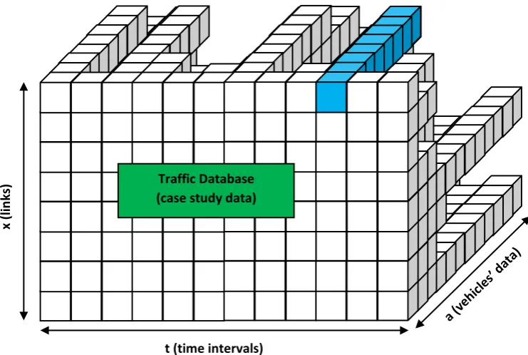
The backbone of both neighbour link methods (NLM) is based on weighting of neighbour links to improve accuracy of the final state estimation/prediction and to fill in the gaps of links with no data by using the data from its neighbours. The global structure of these NLMs is depicted in the figure below. Without going into details here (a complete step-for-step explanation is provided later on in this thesis), it stores newly received traffic data (x) in a traffic database (A). Then the neuron layer (w) finds for each neighbour link, a linear weighting (w) such that this weighting (w) multiplied with the input layer (x) becomes the outputted traffic data (y) of that particular link.

Figure 4:Global structure of the NLM framework

The first big difference between Morita (2011) and Esaway (2012) is the way the neighbourhood space is calculated. Obviously some kind of threshold should be applied as to achieve a reasonable trade-off between accuracy and number of neighbours (which directly influences calculation times. Esaway (2012) makes its selection of neighbourhood links based on correlation in traffic data. The links that show correlating behaviour in the past are assumed to behave the same in the future. Morita (2011) relaxes this assumption and defines the neighbourhood space as just the directly adjacent edges of a link in the network. However, in an urban network it is not necessarily true that directly adjacent links show correlation with the link in question as for example near (signalized) intersections the merging, diverging and yielding of traffic plays a significant role (Tampère, 2011). The approach taken by Esaway (2012) is considered to be intuitively more suitable than the approach of Morita (2011).

The second difference between Morita (2011) and Esaway (2012) is the way of weighting applied to the links in the neighbourhood space. Upon selecting of the neighbourhood space, Esaway (2012) weights the traffic data of the links, by their respective variance. That is; the less reliable a

measurement, the less it is weighted (just as in KF). Subsequently a normalized weighting of these links then yields a final estimation which forcefully lays in between the highest and lowest

measurement on the neighbouring links. Morita (2011) however, weights the traffic data of the links, by using linear regression. By using the traffic data from the link itself as a target, it tries to find any linear weighting of the traffic data on neighbouring links, such that for all times in the traffic database the target is aimed for. This regression approach therefore weights traffic data of

neighbour links that correlate most, relatively higher than neighbour links that correlate less. It can therefore be considered in line with the filtering consequence of the neighbourhood space

correlation approach. As both approaches have merit, combining them and developing them further, is adopted to be a suitable area for further research.

Input Layer (x) Traffic Data Measured

Output (y) Traffic Data Estimated Neuron Layer (w)

Adjustable weights

Historical Database (A) Historic Traffic Data

(18)

18

To make NLM suitable for traffic state predictions, both the neighbourhood space determination and the linear regression parts of NLM must be modified. The neighbourhood space determination can be relatively easily adjusted by determining the correlation between a link and its neighbours not at a set time 𝑡, but at a time in the past, at an exact distance equal to the forecast horizon. The linear regression part can be modified along the same lines, whereas the target of the weighting is not at a time t, but at a time in the future, at an exact ‘distance’ equal to the forecast horizon. With these modifications, the historic traffic database is searched for exactly the idea behind NLM; namely finding which links are indicators for the future traffic state of a link itself.

Lastly the NLM must be made suitable to output flows and densities as well. Essentially the

correlated relationship in velocities also applies to densities. Lower velocities imply higher densities and high velocities imply lower densities. Using the multiplicative relationship between velocity and density gives the flow required. However, density and flow cannot be reasonably be estimated from solely FCD (Seo, 2015) as the fundamental diagram is inherently inaccurate and hard to obtain. For this the fusing of data from FCD and ILDD is to be explored for implantation in the NLM.

For accuracy determination, the model outputs (expected) should be compared with the real world situation (observed). However, the traffic data used to determine this observed situation are inherently noisy and thus not necessarily correct (Snelder, 2015). Treiber (2012) argues that it can only be correct if the full data set serving as reference is so dense that it can be regarded as representing the ground truth. Proposed within this thesis is to use a microscopic traffic model in which an urban network is modelled. This will provide a 100% accurate ground truth and therefore allows unbiased and fair comparison of the performance of the neighbourhood link correlation method. Obviously the downside of this choice is that real world traffic behaviour might be different than the behaviour programmed in the simulation model. For example as the network changes or flow is disturbed, traffic data is noisy (Snelder, 2015), users might be only boundedly rational (e.g. Mahmassani & Chang, 1987).

4.3 Thesis outline

In this fourth chapter, the research subject, context and the challenges that come with urban traffic state estimation and prediction are introduced. In the next chapter, the research objective, research question and scope of this research are presented upon which in the third chapter, the used research methodology is presented.

The subsequent section of this research is divided into three parts. The first part introduces the case study of this research in detail. This first part then yields the ground truth which is used to assess the performance of the NLM. The second part considers the urban traffic state estimation share of this research. In this part the NLM is applied upon the traffic data derived from the case study scenario and subsequently its results are assessed and evaluated. The third part considers the urban traffic state prediction share of this research. Here the modifications to make NLM suitable for prediction are discussed in more detail, after which its’ results are again presented and discussed.

(19)

19

5 Research objective, research question and scope

In this chapter the research objective, the research question and scope of this research are presented.

5.1 Research objective

The main research objective of this master thesis is:

“Design of a traffic state estimation and traffic state prediction method and framework, which by utilizing both floating car- and inductive loop detector data, delivers real-time link-

velocities, -densities and -flows within an urban traffic environment.”

From the previously presented literature review, the theoretically most likely model to perform in an urban network is an improved and redesigned version of the neighbourhood link correlation

methods of Morita (2011) and Esaway (2012). These methods are therefore selected as a starting point for further development of a neighbourhood link method (NLM) framework that fulfils the stated objective.

The first part of the research therefore focusses on designing the NLM framework as to allow enrichment of floating car data considered, by including loop detector data through the process of data fusion. Additionally it needs to be researched how every traffic flow variable can be deduced from the limited availability of both FCD and ILDD. Another objective of research is how the framework should cope with changing traffic conditions within the network. By using a historical database for correlation and weight determination, within day and between day traffic variations provide an additional challenge. The last part assesses and improves the accuracy of the traffic state estimation outputted by analysing sensitivity towards certain choices and finding quick wins to implement in the improved version of the framework.

The second part of the research focuses on the development of the NLM framework towards traffic state prediction. It requires the designed framework from the first part of this research in which the correlation between links is not determined at the same times, but over a certain time horizon (e.g. 5 and 15 minutes). The objective of this second part is then again to assess and improve the accuracy of the traffic state predictions outputted.

5.2 Research question

The main research question of this master thesis is:

“How can a NLM framework best be designed as to deliver both a traffic state estimation and state prediction of all relevant traffic flow variables within an urban network, and how well does it perform in delivering an accurate estimation and prediction for different traffic conditions within the urban network?”

5.3 Scope

(20)

20

Proposed in this research is to work with three design guidelines to frame and limit the direction of the research, to most suitable area for further research identified earlier. The design guidelines proposed are:

1) Every part of the new NLM framework is developed within line of the idea that; patterns in historical traffic data can be used to allow the current traffic state of links to serve as indicators for the current and future traffic state on neighbouring links

2) The developed NLM framework remainsclassifiable as a (hybrid) non-parametric model; 3) The real-time processing power is not forfeited.

(21)

21

6 Research methodology

In this chapter, the research method within this research is introduced. The research method can be divided into three separate parts being; 1) the urban traffic state ground truth, 2) the urban traffic state estimation and 3) the urban traffic state prediction part.

6.1 Part 1: Urban traffic state ground truth

This first part of the research method describes how the ground truth for this research is generated. This designed ground truth remains unchanged throughout this research. It is used to quantify the quality and accuracy of the traffic state estimations and predictions outputted in the second and third part of the research method. The ground truth is – in this context – a database with one minute aggregated velocities, densities and flows on every link in the urban network. A structural overview of the steps executed that lead to the determination of this ground truth is displayed below.

Figure 5: Ground truth traffic state framework

The first step in the ground truth determination process is regarding the choice and set-up of the case study scenario. That is, the network layout, vehicle characteristics, demand and trip distribution are determined. Consecutively it is implemented into the microscopic simulation environment of PARAMICS, upon which the software is run. Each run then yields a full report on real-time loop detector and floating car data. As the floating car data is both 100% accurate and fully covers all the vehicles in the network, the last step is then to aggregate the floating car data into one minute intervals and filling up the ground truth database with average link velocities, densities and flows.

6.2 Part 2: Urban traffic state estimation

The second part of this research method covers the traffic state estimation research method. It is an extension of the previously mentioned ground truth framework with one additional modification. Whereas the ground truth is derived from a 100% penetration rate, the traffic state estimation relies on a lower penetration rate. Dai et al. (2003) conclude that 3% should be a bare minimum for freeway roads and 5% a minimum for so called surface roads. De Vries (2015) shows that with a 5% penetration rate the learning database interpolation already reaches up to 50%-60% of its maximum potential, continuing up to 95% of its max potential at 10% penetration rate.

Therefore a 5% floating car rate is adopted as a starting point. Additionally, the steps of performance results and evaluation and synthesis are included to complete the design cycle. The traffic state estimation outputted is – in this context – a database with one minute aggregated velocities, densities and flow estimations for every link in the previously defined urban network. With the ground truth available (for solely comparative purposes), the state estimations outputted is assessed on accuracy and correlation. Evaluation of these results and more in depth synthesis are then

executed to find and design the best performing NLM variant upon the case study scenario. A structural overview of the whole traffic state estimation framework is presented on the next page.

Case study scenario

Micro-Simulation (PARAMICS)

Real-Time Floating Car Data

Real-Time Loop Detector Data

(22)

[image:22.595.71.520.493.752.2]

22

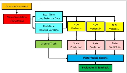
Figure 6. Traffic state estimation framework. Refined expansion of Tao (2012).

The additional steps taken to derive the traffic state estimations thus start with the filtering of the floating car traffic data as a reduction from 100% coverage to 5% is simulated. Additionally another copy is made with 10% penetration rate for review purposes. This data is then inputted in pre-defined different variants of the NLM upon which the state estimations are outputted.

6.3 Part 3: Urban traffic state prediction

The prediction part of this thesis is developed within the more or less same framework as within traffic state estimation. It does however imply some modifications needed to the NLM, because the traffic state is outputted for a time in the future, beyond the most recent available traffic data. For completeness the modified framework is presented below.

Figure 7. Traffic state prediction framework. Refined expansion of Tao (2012).

NLM Variant 1

Performance Results Case study scenario

Ground Truth

Evaluation & Synthesis NLM Variant 2 NLM Variant … State Estimation State Estimation State Estimation NLM Variant a Case study scenario

Ground Truth

(23)

23

PART I

(24)

24

7 The case: Enriched Sioux Falls Scenario

The urban road network chosen for this research is the Enriched Sioux Falls Scenario introduced firstly by Morlok et al. (1973) as a traffic equilibrium network. It has been adopted as a benchmark and test scenario for many publications. Professor Hillel Bar-Gera from Ben-Gurion University of the Negev supplies the open source data for this network (Bar-Gera, 2014). In this chapter the reasoning for choosing this network, as well as the specific network layout, network demand and trip

distribution are discussed.

7.1 Introduction

The considerations leading to the choice for the Enriched Sioux Falls Scenario are based on the following requirements. For this research a small-scale scenario with realistic demand and a high level of disaggregated information is needed to test and demonstrate the urban traffic state

approach. Therefore it is required to find a scenario that is computationally manageable (in this case study setting, without access to optimized soft- and hardware). An additional requirement is that it should be compiled out of open source data in order to ensure both comparability and free public access. Furthermore, the network should resemble a real world scenario, but without necessarily exactly mimicking a particular place. Recently Chakirov (2014) developed an enriched version of the Sioux Falls Scenario with the purpose of mimicking socio-demographic characteristics and spatial distributions. This leads to the development of a scenario which serves for users and developers of agent-based simulation tools as a convenient test-case to serve as a test bed for new software extensions. It therefore aligns with the aim of this thesis. The test scenario used in this thesis is therefore the original Sioux Falls test scenario (Morlok, 1973) expanded in some areas with the

Enriched Sioux Falls Scenario (Chakirov, 2014) to make it suitable for agent-based simulation.

7.2 Network layout & vehicle characteristics

The Enriched Sioux Falls Scenario network in this thesis consists out of the original 24 zones with 24 nodes and 76 links. As the maximum area to be simulated by PARAMICS Discovery v15.0, the

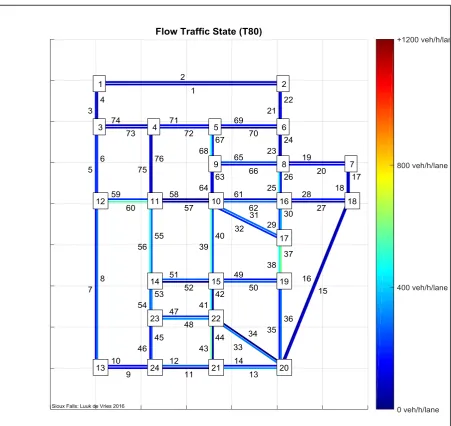
microscopic modelling environment available is capped by license (available for this study) at 10 km² and the original network is of size 17 km², a 25% reduction in node distances is applied (new size = 9,6 km²). The original zone placement on the actual nodes is changed to be on the links directly adjacent to the node, allowing (random) disappearance and appearance of vehicles on links itself, mimicking real world behaviour. The length of all links is set to be equal to the Euclidian distance between nodes, yielding an average link length of 1290 meters. A full map of the network, depicting the nodes, links and road types is displayed on the next page. For the setting of physical road parameters such as road length, number of lanes and a legal speed limit, the two types of road links defined by Chakirov (2014) are copied to PARAMICS. These are highways (2x3 lanes (width: 11m) with an imposed speed limit of 70 mi/h) and urban roads (2x2 lanes (width: 7,3m) with an imposed speed limit of 30 mi/h).

Nodes between highway and urban roads are modelled as simple priority junctions in PARAMICS. The nodes between urban roads are modelled as signalized junctions, with a very simple non-actuated cycle of 30s green time for each opposing direction (allowing left turns in conflict). The cycle times are therefore independent of the actual traffic demand. For node 10 the intersection is a node between five links, and consequently has a total traffic light cycle time of 1m30s. Node 4 is modelled as a signalized junction without any designated priorities. Additionally every link leading to a

signalized junction is equipped with dual inductive loop detectors.

(25)

25

Figure 8: Sioux Falls Scenario network layout used in this research (block size is 0,5 km x 0,5 km)

7.3 Network demand

The starting point for the network demand is an OD-Matrix presented by LeBlanc et al. (1975). This contains a total of 360.600 trips. Chakirov (2014) re-estimates this OD-matrix by designing a household structure with a demographic profile and income distribution using data from census districts in and around the City of Sioux Falls which results in approximately half the total number of trips (d≈0,5). However with the 168.220 trips, the large number of vehicles in the network produces a drop in space-mean flow that persists from 7:30h until 12:00h and therefore yields 4,5h of

(26)

26

7.4 Trip distribution

On the demand side of this Enriched Sioux Falls Scenario, two simple activity chains are introduced to enhance the degree of realism. Instead of a flat uniform trip distribution which will assign the OD-table over time, a more complex trip distribution from Chakirov (2014) is included. The basis for this trip distribution is the two different trip activity chains. The first trip chain is: home – work – home. The second trip chain is: home – other – home. Each trip chain can then be further divided into the trip from home and the return trip.

Chakirov (2014) then adds additional constraints to each separate activity lenient on the

characteristics of: opening hours, work hours and activity durations. Using simple assumptions on normally distributed departure times for work trips and uniformly distributed departure times for secondary activity trips, the network trip distribution for this research is designed with the characteristics of the trip chains are displayed the table below.

Primary (Work) Distribution Mean St. Deviation

1. Home  Work Normal 07:30 15 minutes

2. Work  Home Normal 17:30 15 minutes

Table 2: Primary Activity Trip Distribution Characteristics

Secondary (Other) Distribution Constraints

3. Home  Activity Uniform From 07:45 – 19:45 4. Activity  Home Uniform From 09:00 – 21:00

Table 3: Secondary Activity Trip Distribution Characteristics

For practical implementation in PARAMICS, it is required to determine the profile of distribution, by defining how many of the actual trips are started within time bins of 5 minutes. Because in

PARAMICS the OD-matrix implies only go trips (and not return trips), the OD-matrix is split into two tables, each therefore responsible for half the number of trips. The first table represents the first stage of network trip activities (from home). The second table represents the second stage of

network trip activities (return trip). Using the same key for primary and secondary trip distribution as Chakirov (2014) uses, the ratio between ‘work’ and ‘other’ trip activities is set to 2:1. The profile inputted into PARAMICS is displayed in the figure below in terms of percentage of total trips. These values are to be treated as indicators as the decision to start the trip in PARAMICS is a random decision.

(27)

27

8 Microscopic simulation

The microsimulation software used for this research is PARAMICS Discovery v15.0. It is within this software that the context defined in the previous chapter is drawn up. As previously stated the license available for this research comes with two limits; (1) the maximum traffic area of simulation is maxed at 10 km² and (2) the maximum simulation time is limited to two hours. In this chapter, the simulation characteristics are discussed resulting into 100% correct logs of FCD and ILDD for use in the performance assessment of the interpolation method.

8.1 Simulation Timeframes

The first step concerns choosing one or more interesting timeframes of the simulation. Keeping in mind that the goal of this research is to analyse the performance of the NLM framework in different traffic conditions, the simulation timeframes are chosen such that the most interesting traffic flow characterizations are covered (i.e. traffic breakdown, congestion, recovery). Additionally a timeframe in which solely free-flow traffic conditions are experienced, is added to allow assessment of model performance in free flow conditions and serve as a basis for comparison. Multiple runs of these timeframes with different starting seeds are proposed to mimic between day differences in all simulated periods (not with the intention to find e.g. an average rush hour period). As simulations are time costly and also generate a sizable amount of data, selecting three timeframes of two hour length, and running each simulations a total of 5 times for each of the timeframes is suggested to yield a reasonable trade-off between accuracy and research time.

The rush hour simulation timeframes are set around the mean time of primary trip activities to capture the traffic breakdown, congestion and recovery phases. The two hours of simulation time available, are distributed evenly along the time at which the maximum number of trips are suspected to take place. For the third timeframe an arbitrarily period between morning and evening rush hour is chosen. All periods are considered separately in this research. The simulated timeframes are:

(1) Morning Rush Hour From: 06.30h – 08.30h Peak expected at: 07:30

(2) Evening Rush Hour From: 16.30h – 18.30h Peak expected at: 17:30

(3) Outside (of) Rush Hour From: 12:30h – 14:30h

8.2 Simulation Characteristics

Each period up for simulation is then run a total of five times, to mimic daily variation in traffic due to PARAMICS’ random decision process regarding the release of vehicles, vehicle parameters and choice processes. Each simulation therefore has a unique random generated seed. The output of each simulation are the log files which contain the FCD and ILDD. These make up the ‘traffic data’ used throughout this research. While the simulation itself ran quite fast, averaging 60 times the real time speed, the time consumption for the transferring and saving of the generated traffic data required up to 3 hours per run. A summary of the simulation characteristics and corresponding data sizes are shown in the table below.

Simulation Type Timeframe Runs (Days) ∑ 𝐒𝐢𝐳𝐞 𝐨𝐟 𝐝𝐚𝐭𝐚 Morning Rush Hour 06:30 – 08:30 5 6,89GB

Evening Rush Hour 16:30 – 18:30 5 9,71GB

Low Hours 12:30 – 14:30 5 0,35GB

Table 4: Simulation characteristics

Urban traffic state estimation & prediction