University of Warwick institutional repository: http://go.warwick.ac.uk/wrap
A Thesis Submitted for the Degree of PhD at the University of Warwick
http://go.warwick.ac.uk/wrap/51482
This thesis is made available online and is protected by original copyright.
Please scroll down to view the document itself.
Spatio-Temporal Dynamics in Pipe Flow
by
David Christopher Moxey
Thesis
Submitted to the University of Warwick
for the degree of
Doctor of Philosophy
Mathematics Institute
Contents
List of Figures iv
List of Tables ix
Acknowledgements x
Declaration x
Abstract xii
Abbreviations xiii
1 Introduction 1
1.1 Existing studies . . . 3
1.2 Spatio-temporal intermittency . . . 6
1.3 Outline . . . 8
2 Computational Techniques 10 2.1 Method of Weighted Residuals . . . 11
2.1.1 Collocation Formulation . . . 13
2.1.2 Galerkin Formulation . . . 15
2.2 Spectral/hp Element Methods . . . 17
2.2.1 Diffusion Equation . . . 18
2.2.2 Constructing local modes . . . 21
2.2.3 Common choices for the expansion basis . . . 26
2.2.5 Implementation . . . 32
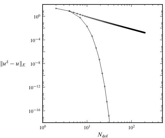
2.2.6 Convergence Properties . . . 35
2.3 Temporal Discretisations for Navier-Stokes . . . 36
2.3.1 Classical high-order schemes . . . 37
2.3.2 Splitting Schemes . . . 38
2.3.3 First-order splitting schemes for Navier-Stokes . . . 39
2.3.4 High-order schemes . . . 41
2.3.5 Pressure boundary condition . . . 42
2.3.6 Stiffly stable schemes . . . 43
2.4 Summary . . . 45
3 Numerical Methods for Pipe Flow 46 3.1 Mathematical Framework . . . 47
3.1.1 Boundary conditions . . . 49
3.1.2 Hagen-Poiseuille Flow . . . 50
3.2 Forcing with Volumetric Flux . . . 52
3.2.1 Constant body forcing . . . 54
3.2.2 Forcing for transition experiments . . . 55
3.2.3 Direct flux condition . . . 56
3.2.4 Green’s function flux forcing . . . 58
3.2.5 TheSemtexSpectral Element Solver . . . 61
3.2.6 Implementation of volumetric flux forcing . . . 62
3.3 Multicore optimisations for parallel Fourier transforms . . . 65
3.3.1 Semteximplementation . . . 66
3.3.2 Multi-core systems . . . 68
3.3.3 Testing and results . . . 70
3.4 Summary . . . 72
4 Transitional Dynamics of Pipe Flow 73 4.1 Resolution requirements . . . 74
4.1.1 Chebyshev-based meshes . . . 75
4.1.2 Spectral-element discretisation . . . 76
4.2 Transitional Dynamics . . . 83
4.2.1 Simulation methodology . . . 86
4.2.2 Identifying turbulence . . . 87
4.2.3 Results . . . 88
4.3 Transition between localised and intermittent turbulence . . . 91
4.3.1 Methodology . . . 91
4.3.2 Results . . . 92
4.4 Onset of intermittency . . . 96
4.4.1 Intermittency factor . . . 97
4.4.2 Laminar lengths . . . 99
4.4.3 Methodology . . . 100
4.4.4 Results . . . 101
4.5 Pattern formation analysis . . . 103
4.5.1 Methodology . . . 104
4.5.2 Results . . . 106
4.6 Conclusions . . . 108
5 Spreading turbulence in pipe flow 110 5.1 Decay studies . . . 111
5.1.1 Lifetime statistics . . . 114
5.1.2 Current state of lifetime statistics . . . 117
5.2 Puff splitting . . . 118
5.2.1 Methodology . . . 120
5.2.2 Results . . . 125
5.3 Directed percolation . . . 128
5.3.1 Bond percolation . . . 129
5.3.2 Universality and connections to pipe flow . . . 131
5.4 Critical point . . . 134
5.5 Conclusion and Discussion . . . 137
6 Summary 139
List of Figures
1.1 Contours of the streamwise velocity through circular cross-sections of a pipe. The left-hand image depicts a laminar flow in which the fluid is steady and unchanging in time. This contrasts with the right-hand image, which is a snapshot of a highly fluctutating turbulent flow at ReD3;000. . . 2
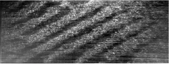
1.2 Visualisations of turbulent and intermittent flow in a cross-section of an
LD25Dpipe. Red indicates high values of the vorticity!D r uand
blue low values. . . 5 1.3 Laminar-turbulent bands in experiments of Couette flow at ReD358, taken
from Prigentet al. (2003). . . 7
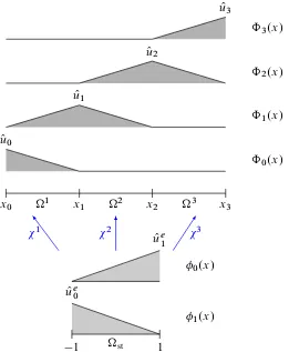
2.1 Global and local expansion bases ˆk and k for a three-element finite
element expansion.eis the linear projection mapping the standard element sttoe. . . 22
2.2 Typical modal and nodal expansion bases defined inside the standard element
st. . . 27
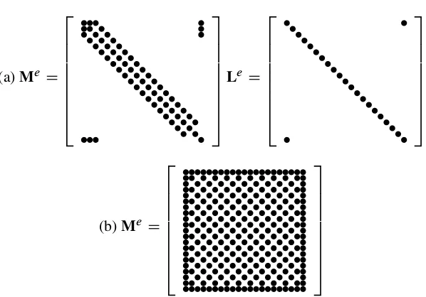
2.3 Elemental mass matrixMeand Laplacian matrixLefor different choices of
elemental modesp at polynomial orderP D20. Dots indicate non-zero
entries. (a) The most common choice for a modal expansionp D p. (b)
The result of changing the interior modes seen in (a) toJp 13;3./. . . 30
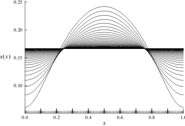
2.4 Solution to the diffusion equation using the parameters outlined in section 2.2.5 with the initial conditionu.x/Dx.1 x/for.x; t /2Œ0; 1. The
distribution of Gauss-Lobatto-Legendre (GLL) points inside each element can be seen along thex-axis. . . 33
2.5 Logarithmic plot of the errorEf measured using the energy norm forh- and
3.1 Average velocity profiles for laminar (left) and turbulent (right) flows through the cylindrical pipe, where averaging is performed over the axial and az-imuthal directions. These profiles are normalised so that in each case the flowratesR
C udS are equal. . . 51
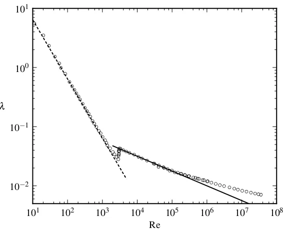
3.2 Schematic diagrams depicting flow being driven using (a) constant pressure gradient and (b) constant volumetric flux. . . 53 3.3 Friction factorfor fully developed pipe flow at a variety of Re. Dashed
line indicates the laminar Hagen-Poiseuille friction lawD64=Re and the
solid line the Blasius lawD0:3164Re 1=4. Data points are taken from
the experimental results of McKeonet al. (2004) and show the transition between the two laws. . . 55 3.4 Geometry of the backwards facing step, for which the Stokes field possesses
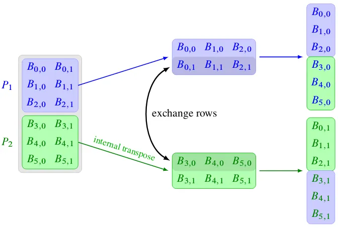
a singular point at the step edge. . . 60 3.5 Exchange procedure forQD2processors overNx D6planes. . . 67
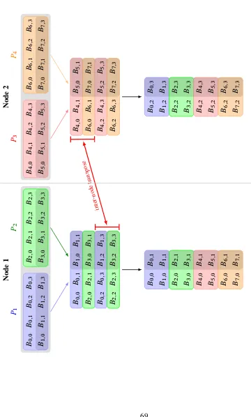
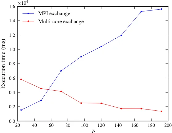
3.6 Shared memory implementation of the algorithm of figure 3.5 for two nodes, each possessing two processes. The first step involves each process perform-ing the same local block transpose, where the blocks are written into a large shared memory block and interleaved with the data from the other processor. A single process on each machine then performs the all-to-all transpose. . . 69 3.7 Execution time in milliseconds as a function of the number of processorsP
for the originalSemtexexchange (blue) and new multi-core exchange (red). 71
4.1 Examples of different types of mesh construction for the two-dimensional circular cross-section of the pipe. Spectral-element meshes use polynomial orderP D12. Elements which are filled in indicate the placement of GLL
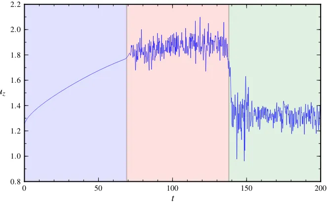
nodal points. . . 77 4.2 Trace of the axial velocityu.0; t /for the instigation of turbulence in a pipe
of length L D 20D. The figure is split up into three regions: (a) initial
deformation of the turbulent profile; (b) onset of instabilty; (c) transition to statistically steady turbulent flow. . . 80 4.3 L1error of the near-wall axial velocityu+zfor various polynomial ordersP
4.4 Axial component of the near-wall velocityu+zin a full-turbulence simulation
at ReD3000using two different types of meshes. . . 83
4.5 Schematic traces of the axial velocityufor a puff (left) and slug (right) along
the pipe axisxadvected from left to right. Leading edges (LE) and trailing
edges (TE) are noted on each figure.umaxsignifies the maximum attainable
laminar velocity (equal to 2 ifU D1). . . 84
4.6 Dynamics of transitional flow from simulations of aLD125Dpipe. The
central plot shows a space-time diagram with the streamwise direction hor-izontal and time increasing vertically upwards. The value of Re changes as indicated on the right. The magnitude of the transverse velocity q is
sampled along the axis of the pipe and visualised in a frame moving at the average fluid velocity:q.x U t; t /. Colours are such that light corresponds
to turbulent flow and black corresponds to laminar flow. Below and above are flow visualizations in vertical cross-sections through the pipe at the initial and final times, and over the25Dstreamwise extents indicated by arrows. . 89
4.7 Simulations highlighting the difference between localised turbulence at ReD2;250(left) and spatio-temporal intermittency at ReD2;350(right). . 93
4.8 Streamwise velocityuandy-component of the transverse velocityvfor the
final state of figure 4.7 at ReD2;250(top) and ReD2;350(bottom). . . . 94
4.9 Intermittency functionI.x; tI110 2/for velocity traces of a single puff
(top) and multiple puffs (bottom). . . 98 4.10 Visualisation of the laminar length distributionL.`/for in a pipe of length
LD25Dat ReD2;200(left) and ReD2;600(right). . . 100
4.11 Intermittency factor(top) and the variance of the laminar length distribution (bottom) for indicated Reynolds numbers. Each curve represents a different
threshold, fromqD410 3(top curve) toqD110 2(bottom curve)
in increments of 210 3. . . 102
4.13 Normalised single-point velocity pdfs for ReD2;350, 2,400, 2,450, 2,500,
2,600, 2,800 and 3,000, as indicated by labels and alternating line types. For Re>2;700, the distributions are nearly Gaussian, and for Re62;600the
distributions are non-Gaussian. . . 104 4.14 Above (a-c):Two-dimensional approximations of the complex pdf1.r; /
of first-order Fourier modes.Below: Cross-sections of1.r; /at D0for
ReD2;200(bottom curve),2;300,2;400,2;500and2;800(top curve), as
indicated by arrows and alternating line types. . . 107
5.1 Spatio-temporal dynamics of puff splitting in a L D 100D domain at
ReD2;350. The turbulence intensityq.x; t /as defined in equation (4.1) is
visualised in a frame of reference moving at speedc D0:914U. The white
dashed line indicates the splitting time detected by the criterion of section 5.2.1. . . 119 5.2 Splitting dynamics in a pipe of lengthLD200Dat ReD2;350. Turbulence
intensityq.x; t /as defined in equation (4.1) is visualised in a frame moving
atc D0:924U. . . 121
5.3 Snapshots of the streamwise vorticity!x through cross-sections of anLD
50Dpipe at ReD2;350as a puff splits. Positive and negative vorticity are
denoted by blue and red respectively; black areas represent!x D0. Att D0
(bottom image), Re is changed from 2,100 to 2,350, and further snapshots are taken att D50; 138; 198with the snapshot att D438showing the final
two-puff configuration. . . 122 5.4 Schematic drawings depicting criterion used to determine splitting times.
Shaded rectangles indicate the region around the primary peak of the signal to be ignored, of widthdminD20D. . . 123
5.5 Initial condition number i against detected splitting time ti for samples
5.6 Survival functionsS.t /for Re D 2;300(top) and Re D 2;350 (bottom). .n; r/ D .90; 51/ and .95; 90/ samples are obtained respectively using Semtex(DNS1) and the code of Willis & Kerswell, 2009 (DNS2, courtesy of
Marc Avila). Dashed line represents the curveS.t /DexpΠ.t t0/= .O Re/,
and shaded areas represent the 95% confidence interval associated with each simulation. . . 126 5.7 Directed bond percolation on a (1+1)-dimensional square lattice utilising
periodic boundary conditions, where the percolation direction (time) is vertically upwards. Active and inactive sites are denoted by black and white dots respectively. Open bonds are represented by solid lines, and closed bonds by dashed lines. Numbers along the bottom correspond to spatial locationsi. . . 130
5.8 Examples of critical behaviour in directed bond percolation usingN D500
sites over t D 2;000 timesteps. Figures along the top row start with a
configuration possessing a single active site, and those below use a random initial configuration. . . 131 5.9 Space-time figures demonstrating a relationship between directed percolation
and pipe flow. In each case, the initial condition is an isolated puff, and Re is instantaneously set to 2,700 (top) and 1,700 (bottom). . . 133 5.10 Characteristic lifetime as a function of Reynolds number for an isolated
puff. Coloured points represent experimental data (courtesy of Kerstin Avila, Alberto de Lozar and Björn Hof), and solid black triangles those obtained fromSemtex(DNS1) and a hybrid spectral finite-difference code (DNS2).
The dashed line denotes the super-exponentially increasing fit for mean decay times, and the solid line the decreasing fit for mean splitting times. The crossover point at Rec D2;040˙10, determines the transition between
List of Tables
4.1 Axial resolution requirements for the pipe expansion experiment of section 4.3.1 for various domain lengthsL. . . 92
5.1 Data obtained from DNS1 of the characteristic splitting time as a function
of Reynolds number, where each simulation observes r splittings from ninitial samples. t1denotes the first observed splitting time, andtmaxthe
Acknowledgements
Firstly, I am incredibly grateful to my supervisor, Prof. Dwight Barkley, for his encour-agement and support throughout the last four years. There is no question that without his invaluable advice, insight and knowledge this thesis would never have seen the light of day, and I feel enormously lucky and privileged to have had him as my supervisor.
My immense thanks go to Kerstin Avila, Alberto de Lozar, Marc Avila and Björn Hof of the University of Göttingen for their collaboration with us on the results of chapter 5. Many of the important conclusions drawn in this chapter would not have been possible without them. I also thank Prof. Hugh Blackburn for providingSemtex, the code used throughout
this thesis to generate all of our results. I am also grateful for the comments of my examiners, Prof. Rich Kerswell and Prof. Sergey Nazarenko, which have greatly improved areas of this thesis.
This work would also not have been possible without the hundreds of thousands of computer hours provided by the University of Warwick Centre for Scientific Computing, HECToR and GENCI-IDRIS, and I would like to thank the staff and adminstrators for their hard work maintaining these systems. I am also grateful to the Engineering and Physical Sciences Research Council for providing funding throughout my postgraduate studies.
Throughout both my undergraduate and postgraduate degrees, many people both inside and outside the Mathematics Institute at Warwick have made my time here unforgettable. Unfortunately I simply do not have the space to list you all! In particular however, I am incredibly grateful to have had the company of my fellow compatriates in B2.39 throughout the years: David White, Simon Cotter, Chris Cantwell, Damon McDougall, Tom Ranner and Andrew Duncan. All of you have been there to help too many times to mention, so thank you all! Many thanks go to Mark, Erin, Rod and Robby for providing many fun evenings and being around when I needed an ear.
Declaration
Abstract
When fluid flows through a channel, pipe or duct, there are two basic forms of motion: smooth laminar flow and disordered turbulent motion. The transition between these two states is a fundamental and open problem which has been studied for over 125 years. What has received far less attention are the intermittent dynamics which possess qualities of both turbulent and laminar regimes. The purpose of this thesis is therefore to investigate large-scale intermittent states through extensive numerical simulations in the hopes of further understanding the transition to turbulence in pipe flow.
We begin by reviewing the spectral-element code Semtexwhich is used to perform the
simulations. We discuss modifications to this code to impose a constant flowrate to the flow through a pipe and to improve the computational efficiency on certain multicore architectures. We then move on to examine the reverse transition from turbulence to laminar flow in a long, 125 diameter periodic pipe, which unlike the forward transition does not depend on finite-amplitude perturbations to the flow and thus captures the natural dynamics contained within the transition. The Reynolds number Re is reduced from ReD2;800to ReD2;250over
a long timescale, and by investigating the resultant spatio-temporal dynamics we discover that the transition can be characterised by three fundamentally different states separated by two Reynolds numbers. Below Rec .2;300, turbulence takes the form of equilibrium puffs
which eventually decay. Above Rei 2;600, flow remains uniformly turbulent throughout
the domain. Between these two values, the dynamics are an intermitent mixture of both turbulent and laminar regimes which take the form of unsteady alternating laminar-turbulent bands.
Finally, we concentrate on finding a more exact value for Rec, which marks the onset
Abbreviations
CFL Courant-Friedrichs-Lewy (condition) CPU Central Processing Unit
DFT Discrete Fourier transform DNS Direct numerical simulation DP Directed percolation
iid Independent identitically distributed FFT Fast Fourier transform
GLL Gauss-Lobatto-Legendre (collocation points) LE Leading edge
LHS Left hand side
MLE Maximum likelihood estimator MPI Message Passing Interface ODE Ordinary differential equation PDE Partial differential equation PDF Probability density function Re Reynolds number
Chapter 1
Introduction
Fluid flows play an important role in a wide range of problems in science and engineering, be it in hugely complex atmospheric dynamics with vast numbers of degrees of freedom, the analysis of blood flowing through veins and capilliaries or using mixing properties to design efficient heat exchangers. The motion of a fluid is inherently complex, and in many cases appears random, which makes it both hard to predict and difficult to analyse. Understanding these dynamics has proven to be one of the most important and exhaustively studied problems in mathematics, physics and engineering, spanning more than two centuries of detailed investigation. Of all of the countless scenarios in which we can study fluid flow, in this thesis we consider one of the simplest, oldest and most puzzling – the flow of a fluid through a straight, cylindrical pipe.
In general, we may classify a fluid flow into three distinct states. Inlaminarflows, motion is smooth and regular, and often has symmetry in simple geometries. Inturbulentflows, the fluid exhibits highly irregular and unpredictable motion which is usually characterised by the interaction of unsteady vortices over a wide variety of length scales. Figure 1.1 demon-strates the striking difference between these two states in pipe flow. One of the classical fluid dynamics problems is to understand precisely how and why turbulence arises from laminar behaviour. Key to this problem is the third type of flow, usually calledintermittent
Figure 1.1:Contours of the streamwise velocity through circular cross-sections of a pipe. The left-hand image depicts a laminar flow in which the fluid is steady and unchanging in time. This contrasts with the right-hand image, which is a snapshot of a highly fluctutating turbulent flow at ReD3;000.
The transitional dynamics of pipe flow were first investigated in the pioneering work of Reynolds (1883a,b) which demonstrated the existence of a relationship between the onset of turbulence and a dimensionless parameter, known today as the ubiquitousReynolds number
ReD U D :
HereDis the diameter of the pipe,is the fluid’s kinematic viscosity andU is the mean
(bulk) velocity of the flow. At low Re, the viscous effects of the fluid outweigh the inertial forces, causing disturbances to decay and the flow to revert to a laminar state. As Re increases, the balance of inertial and viscous forces changes so that a perturbation applied to the fluid grows in strength and eventually gives rise to a turbulent flow. This concept also translates to a number of other geometries, such as the flow between two solid planes or over a backwards-facing step, and as such the Reynolds number forms a key concept in fluid dynamics.
Curiously however, after being investigated for over 125 years, the question of a finding a
1.1 Existing studies
Pipe flow, and fluid flow in general, has proven to be very resilient to mathematical analysis. Assuming the fluid is Newtonian and incompressible, the flow is governed by the Navier-Stokes equations
@u
@t C.u r/uD rpCr
2
u; (1.1)
r uD0; (1.2)
whereuis the fluid velocity andpis the pressure field. One of the simplest mathematical
tasks is to determine whether, given a smooth initial condition, this partial differential equation (PDE) has a smooth solution for all timest > 0. The difficulty of this problem
is particularly emphasised by the fact that it remains one of the six unsolved Clay Institute Millennium challenges, for which a solution commands a one-million dollar reward.
In pipe flow, the simplest analytic solution one may examine is that of laminar flow, seen in figure 1.1, which may be derived exactly from equation (1.1) (see section 3.1.2). A common mathematical technique for determining bifurcations in non-linear systems of PDEs which depend upon a parameter is to consider infinitesimal perturbations of a known solution and linearise the resulting equations of motion. However, even this relatively straight-forward approach has yielded few analytic results. Joseph & Carmi (1969) showed that any disturbance introduced to the fluid for Re < 81:49decays to the laminar profile.
Most evidence suggests that, in fact, laminar flow is stable to these perturbations atanyRe. Whilst this has not been proven, Meseguer & Trefethen (2003) demonstrated this through direct numerical simulations (DNS) of the linearised Navier-Stokes equations and observed stability as high as ReD107. There are also a number of proofs in cases where restrictions
on the type of perturbation are applied. For example, as stated by Crowder & Dalton (1971), the hydrodynamic stability of laminar flow subject to axisymmetric perturbations may be traced back to Sexl (1927), and some sixty years later stability under these conditions at any Re was proven by Herron (1991).
and later Pfenniger (1961) demonstrated laminar flow up to ReD105. However, the pipe
must be properly isolated from outside vibration and temperature fluctuations to achieve laminar flow at such high Reynolds numbers. The shape of the inlet must also be very carefully designed to avoid unnecessary perturbation of the flow. Given a pipe capable of sustaining laminar flow, the original idea behind Reynolds’ work is the concept of a critical Reynolds number, Rec, below which perturbations that are deliberately introduced to the
flow eventually decay and turbulence cannot be sustained.
Most studies of turbulence expand on this concept by introducing finite-amplitude pertur-bations to the fluid, and observing how the flow evolves over time at different values of Re. Upon introduction of the perturbation, one may observe two outcomes: the flow may either transition to turbulence, or instantly revert to a laminar state. The regime that is observed depends on the amplitude of the perturbation, and the critical threshold needed to trigger transition obeys a power law as a function of Re (Darbyshire & Mullin, 1995, Hofet al., 2003, Peixinho & Mullin, 2007). However, the amplitude of the perturbation alone does not govern Rec. Assuming that the perturbation is sufficiently strong, Reynolds’ original
experiments noted that around the transition point one typically observes isolated turbulent ‘flashes’ which grow and split to contaminate the downstream flow, and are separated by regions of laminar flow. Wygnanski & Champagne (1973) demonstrated that these flashes can be classified into two separate structures, which they deemedpuffsandslugs. Puffs consist of a small pocket of turbulence which is embedded in the surrounding laminar flow, and are found close to the suspected transition point at Re2;000. Slugs are the high-Re equivalent
found past Re& 2;700which rapidly grow to fill the whole pipe and cause turbulence to
spread downstream of the perturbation. Understanding the transition to turbulence then hinges on observing the dynamics of puffs (and to a lesser degree slugs) and determining the mechanisms that govern their behaviour.
Figure 1.2: Visualisations of turbulent and intermittent flow in a cross-section of anLD 25Dpipe. Red indicates high values of the vorticity!D r uand blue low values.
of studies (Faisst & Eckhardt, 2004, Peixinho & Mullin, 2006, Hofet al., 2006, Willis & Kerswell, 2007, Hofet al., 2008, de Lozar & Hof, 2009, Kuiket al., 2010). The most recent statistical analysis of Avilaet al. (2010) however, presents the strongest evidence yet that puff lifetimes remains finite at any Re, and thus it is impossible to determine the critical Reynolds number from considering the mean lifetime of puffs alone.
Another line of investigation which may aid in understanding the mechanism behind the onset of turbulence has been the discovery of unstable coherent structures which are alternative to that of the laminar profile. The work of Faisst & Eckhardt (2003) and Wedin & Kerswell (2004) confirmed that travelling waves (TWs) – symmetric structures which move through the pipe with constant wave speed – exist within the framework of pipe flow, and were later shown to exist experimentally by Hofet al. (2004). Further studies including those of Pringle & Kerswell (2007), Willis & Kerswell (2008), Willis & Kerswell (2009) and Pringleet al. (2009) have greatly expanded the number of known TW solutions. From a dynamical systems standpoint then, laminar flow is a globally stable solution below Rec, and
the perturbation of the fluid leads to a solution which wanders between the unstable solutions in phase space before eventually returning to laminarity. Above Rec the flow undergoes a
1.2 Spatio-temporal intermittency
The common theme throughout the majority of studies outlined in the previous section is the forward transition from laminar flow to turbulence, where observations are not only dependent on Re but on both the type of perturbation used to trigger transition and its amplitude. However, intermittent states, such as those seen in the experiments of Rotta (1956), have rich spatio-temporal behaviour which has for the most part not been investigated. The difference between fully turbulent flow and intermittent states is highlighted in figure 1.2; the top pipe shows a simulation at ReD3;000, where the flow is uniformly turbulent
and structure lengths are roughly uniform throughout the domain. At lower values of Re (here2;300), areas of laminarity begin to appear, with structures growing considerably in
size.
One line of research that is emerging in the investigation of critical Reynolds numbers is the consideration of alternating turbulent-laminar bands depicted in figure 1.3 which form within the flow. It has been established that in plane Couette flow (Prigent et al., 2002, 2003, Barkley & Tuckerman, 2005, 2007), counter-rotating Taylor-Couette flow (Prigent
et al., 2002, 2003), and plane Poiseuille flow (Tsukaharaet al., 2005), near transition the system can exhibit a remarkable phenomenon in which turbulent and laminar flow form persistent alternating patterns on scales very long relative to both wall separation and the spacing between turbulent streaks. While the origin of these patterns remains a mystery, they are intimately connected with the lower limit of turbulence in shear flows. Key to the investigation of these states is the consideration of thespatio-temporalaspects of the flow. Investigating these states in pipe flow is a more challenging endeavour, mostly due to the strong advection of fluid down the length of the pipe.
The fundamentally different approach taken in this thesis then is to investigate the intermittent dynamics found in thereversetransition from turbulent to laminar flow, as opposed to most previous work which has focused on the forward transition problem. In doing this, we hope to observe the formation of turbulent-laminar bands, and examine how these bands evolve over time in order to determine their role in the transition process.
Figure 1.3: Laminar-turbulent bands in experiments of Couette flow at ReD 358, taken
from Prigentet al. (2003).
involves a sharp expansion in the channel or pipe causing the flow to abruptly transition. This differs significantly from the approach we take here, in which Re is slowly and deliberately reduced over a long timescale in order to carefully examine the structures which form within the flow. Indeed, for the most part we are not interested in the full relaminarisation of the fluid, but in the states just before the transition. To replicate this process in an experimental setting demands pipes of many thousands of diameters in length, and also the ability to observe the velocity and pressure fields throughout the length of the pipe.
To overcome these limitations, we shall focus on performing a series of detailed computa-tional experiments of pipe flow. Eggelset al. (1994) performed the fully-resolved turbulence computations in a pipe of lengthLD5D. Later work by Shanet al. (1999) used a spectral
element code to simulate puffs and slugs and expanded these domains to a much larger
L D16D; however the computations here suffer from under-resolution in the axial
di-rection, especially in the simulation of slugs at Re D 5;000. Only in the last decade has
computing technology advanced to the point where, for example, puffs and slugs can be faithfully represented. Faisst & Eckhardt (2004) examined decay in a pipe of lengthLD5D
with better resolution, but too short to fully encompass a single puff. More recently however, Willis & Kerswell (2007), Pringle & Kerswell (2007) and Willis & Kerswell (2008) employed the use of an efficient hybrid finite-difference–spectral solver in domains of up to length
LD50Dand are the first examples of fully-resolved simulations in domains large enough
1.3 Outline
In chapter 2 we introduce the numerical techniques which will be used to perform the DNS of pipe flow. We begin by studying spectral-type methods, which describe a class of algorithms possessing exponential convergence of approximations to solutions of a PDE. The main goal of this chapter is to introduce the spectral element method, which combines the geometric flexibility of a finite element method with spectral-type accuracy. To motivate this, we show the implementation of the method for the one-dimensional diffusion equation. Finally, a number of high-order splitting schemes for the evolution of the Navier-Stokes equations are introduced, along with a discussion of the high-order pressure boundary condition which is needed to make these methods numerically stable.
Chapter 3 introduces the mathematical framework in which pipe flow is studied and the laminar equations of motion are derived. Following this, two numerical techniques useful for the study of pipe flow are outlined. The first is an algorithm which allows the flow to be driven by specifying a constant volumetric flux. This is particularly applicable in transitional flow problems as it prevents deviations in the mean flowU and thus fixes Re.
An efficient Green’s function method is derived as a part of the mathematical formulation, meaning that unlike other methods the flowrate can be imposed exactly at each timestep. We then introduceSemtex, the code which is used in later chapters to perform pipe flow
simulations, and show how this flux condition can be implemented. Finally, we outline the second numerical method which provides optimisation for the parallelisation ofSemtexin
the case where the underlying system architecture makes use of massively multi-core nodes.
Chapter 5 focuses on puffs and the role that they play in the transition process. Whilst the precise distribution of puff lifetimes has remained a contentious issue for a number of years, recently it was conclusively shown that the lifetime of a puff remains finite for all Re (Avila
Chapter 2
Computational Techniques
The investigation of many interesting physical systems usually leads to a mathematical repre-sentation involving a non-linear dynamical system, often in the form of a partial differential equation. In almost every case, it is impossible to explicitly derive non-trivial solutions to these systems, and so the development of techniques which allow us to approximate solutions is of great significance to both mathematicians and others in the physical sciences. Typically, these approximations involve the use of complex algorithms, and so we turn to computers in order to implement them through numerical means.
With fluid flows being amongst the most throughly examined non-linear systems, there are a vast array of numerical methods which can be used to approximate flow fields. Notably, the emphasis throughout this thesis is on obtaining solutions through direct numerical simulation; i.e. the direct integration of the partial differential equations governing the flow, at a scale which accurately reproduces all of the key features contained within it. The goal of this chapter is to outline a small number of these numerical methods. In the next chapter, we describe how these methods can be used in the setting of pipe flow.
We begin with a study of the method of weighted residuals, a generic framework which allows us to employ a wide variety of methods in order to computationally solve problems. In particular, we focus onspectralmethods, which are generally known for their excellent convergence properties and accurate solutions. We study these methods in two different contexts: collocationmethods rely on a fixed discretisation of the spatial domain, whereas
without relying on explicit knowledge of the domain.
The bulk of this chapter concentrates on examining finite element methods, which are typically used to study problems defined in complex geometries. The inspiration behind this technique is to break the domain up into disjoint elements on which the equation can be more readily solved, and then recombine the contribution of each to produce the global solution according to certain constraints on elemental boundaries. In particular, we focus on thespectral/hpelement method, which combines spectral-type accuracy with the geometric flexibility of finite elements, and is the method comprising the vast majority of the numerical results in later chapters. To demonstrate this scheme, we introduce the concepts necessary to formulate a one-dimensional implementation and use this to numerically solve the diffusion equation.
Finally, having made an overview of the schemes which are generally used in the spatial discretisation, we introduce a variety of timestepping schemes. Given the high-order spatial accuracy afforded by the discretisations mentioned above, we discuss the possible algorithms which can be employed to increase the accuracy of approximate flow fields as the equations of motion are integrated over time.
2.1 Method of Weighted Residuals
The basis of any spectral method relies heavily on the method of weighted residuals. It is well known that periodic functions onŒ0; 2which belong to the set
L1.Œ0; 2/D
²
f WŒ0; 2!R
ˇ ˇ ˇ ˇ
Z 2
0 j
f .x/jdx <1
³
can be written in terms of summations of infinitely many orthogonal functions – for example, in Fourier analysis, functions are represented in terms of trigonometric functions. In terms of numerical analysis, the basis of a spectral method is to use a truncated series containing
finitelymany functions in order to obtain an approximation to the function.
Consider a time-dependent linear differential equation over a domaingiven by
and assume that the function can be accurately approximated by a partial expansionuıin
terms ofmodesk:
u.x; t /uı.x; t /D
N 1
X
kD0 O
uk.t /k.x/: (2.2)
In general, an approximation ofuby finitely many modes will not be exact, so we expect to
find some difference betweenuanduı. Substituting (2.2) into (2.1), we therefore obtain a
non-zero functionRknown as theresidualwhich is dependent uponuı,
L.uı/DR.uı/:
In the approximation (2.2), there is no distinct way of choosing the weightsuOk. However,
by placing restrictions on the form of the residual, we can reduce the problem to solving a system of ordinary differential equations in terms ofuOk. The choice of restriction we use
leads to a variety of different numerical schemes. First however, we need a definition in order to define the notion of orthogonality.
Definition 2.1.1 (L2 inner product). The L2 inner product .;/L2 for functions f; g W
!Cis defined as
.f; g/L2 D
Z
f .x/g.x/dx
wherezdenotes the complex conjugate ofz2C.
One way to restrict the residual is through use oftest functionsvj.x/which are orthogonal
toRunder.;/L2;
.vj; R/L2 D0; j D0; : : : ; N: (2.3)
Two of the most popular choices for the test functions produce thecollocationandGalerkin
2.1.1 Collocation Formulation
For the collocation method, we choose the test function to be a Dirac delta functionvj.x/D
ı.x xj/, where thexj 2are a set of points known as thecollocation points. Substituting
this into (2.3), we obtain
Z
R.x/ı.x xj/dxD0
and so by definition,R.xj/D0. The differential equation is therefore satisfied exactly at
each collocation pointxj.
Depending on the choice of modal functions, there are various subclasses of collocation methods. Typically, one chooses amongst common orthogonal bases depending upon the type of boundary conditions to be applied on the domain. In this thesis, we will concentrate on using collocation methods with periodic boundary conditions, on the intervalDŒ0; L.
Under these conditions, the predominant choice of modal function is formed from trigonomet-ric basis functions, in which case we obtain theFourier collocationmethod.is discretised
into a uniform grid ofNC1pointsxj DjL=N; j 2 ¹0; : : : ; Nº, and modes are taken to
bek.x/Deiˇkx whereˇk D2k=N. These functions form an orthogonal set, since
N 1
X
jD0
eiˇkjeiˇlj DN ı
kl D
´
0; k¤l;
N; kDl:
AssumingN is even, rewriting (2.2) in the form
Uj.t /WDuı.xj; t /D
N=2
X
kD N=2C1 O
uk.t /eiˇkj;
and using the orthogonality relation, we can determine the weightsuOkvia thediscrete Fourier transform(DFT)
O
uk D
1 N
N 1
X
jD0
Uj.t /eiˇkj
The DFT is the obvious analogue of the continuous transform,
O
f .k/D
Z
R
which itself is useful for solving PDEs analytically, mostly due to the transform of a differen-tial operator:
b
dfdx.k/D
Z
R
f0.x/ei kxdxDi k
Z
R
f .x/e i kxdx Di kf .k/O
In the discrete case, a similar identity holds:
@uı @x ˇ ˇ ˇ ˇ ˇxDx
j
D @x@
N=2
X
kD N=2C1 O
uk.t /ei kx
xDxj
D
N=2
X
kD N=2C1
i kuOk.t /eiˇkj
so differentiation in spectral space is equivalent to multiplying each modeuOkbyi k. Notice
that the Fourier modes are periodic, since
O
ukCN D N 1
X
jD0
UjeiˇkCNj D N 1
X
jD0
Ujeiˇkje2ki D N 1
X
jD0
Ujeiˇkj D Ouk:
This property therefore requires the approxmiationuıto also be periodic. Also, in the case
where the data pointsUj are real, we may exploit additional Hermitian symmetry so that we
need only calculateuOk fork>0:
O
uk D N 1
X
jD0
Ujeiˇkj D
N 1
X
jD0
Ujeiˇkj D
N 1
X
jD0
Uje iˇkj D N 1
X
jD0
Ujeiˇ kj D Ou k:
2.1.1.1 Non-linear Problems
Whilst the Fourier collocation method is extremely practical for linear problems, it be-comes far less efficient when dealing with non-linear operators. For example, the spectral discretisation of the non-linear term
u@u @x
results in anN N matrix in general, and is therefore not practical to use when combined
performed.
Whilst in theory this procedure is more efficient, this process can only be considered if the transform technique is sufficiently quick to avoid the computational overheads. In addition, the multiplication in physical space leads to the appearence of aliasing errors in the solution. However, for a basis of Fourier functions in one dimension, both of these problems are easily overcome with use of the Fast Fourier Transform (FFT) and the classical 3/2 rule to dealias solutions (Canutoet al., 1988).
This problem is investigated in further detail in section 3.3, where we consider a joint discretisation in which a three-dimensional domain is decomposed using the Fourier pseudo-spectral method in a single dimension and a pseudo-spectral element scheme used in the remaining two. For large-scale problems requiring parallelisation, it is relatively easy in terms of implementation to decompose the domain over the Fourier modes. However, the transform between spectral and physical space commands large communication overheads, and thus we examine ways in which the transform can be optimised in the case where the underlying architecture comprises massively multi-core machines.
2.1.2 Galerkin Formulation
We motivate the study of Galerkin schemes by considering an example of the one-dimensional Poisson equation on the intervalDŒ0; 1, whereLD@2xxCg, giving the equation
@2u
@x2 Cg.x/D0 (2.4)
In order for this for the problem to be well-posed and thus have a unique solution, we must impose boundary conditions. We consider both Dirichlet and Neumann boundary conditions for this problem to show how both types are implemented in a Galerkin setting, so that
u.0/DgD;
@u
@x.1/DgN (2.5)
wheregD andgN are constants. With both equations (2.4) and (2.5), the problem is said
arbitrary test functionv.x/and integrate, giving the integral equation
.v;L.u//L2D
Z 1
0
v
@2u @x2 Cg
dxD0: (2.6)
Assuminguandvare sufficiently smooth, we may then integrate by parts to obtain
Z 1
0
@v @x
@u @x dx
„ ƒ‚ …
a.u;v/ D
Z 1
0
vf dxC
v@u @x
1
0
D
Z 1
0
vf dxCv.1/gN
„ ƒ‚ …
f .v/
v.0/@u @x.0/:
We make the further assumption thatg.x/and thusf is well behaved in the sense thatf .v/
remains finite. Therefore we restrict the choice of solutionsuto those lying in a trial space X, where
X D ¹uju; u02L2./; u.0/DgDº:
The space of possible test functionsV is defined similarly, so that
V D ¹vjv; v02L2./; v.0/D0º:
With these choices, the problem is now said to be inweak form, and the weak solution to the original equation translates to the problem of findingu2X such that
a.u; v/Df .v/; 8v2V:
This problem is still infinite dimensional, and therefore not solvable through computational means. To overcome this, we take finite-dimensional subsets ofX andV, denoted byXı
andVı respectively. The problem then becomes to finduı 2Xısuch that
a.uı; vı/Df .vı/; 8vı 2Vı:
homogeneous partuH 2Vı and a known componentuD 2Xıso that
uı DuH CuD
whereuH.0/ D0 anduD.0/ D gD. This completes the classical Galerkin formulation,
under which we choose the test space and trial space to be the same. Assuming certain properties ofa, one can now apply the Lax-Milgram theorem (Lax & Milgram, 1954) to
guarantee solutions to the problem.
2.2 Spectral/hp Element Methods
Either of the collocation or Galerkin methods defined above, when coupled with sensible choices of modes such as the Fourier scheme seen earlier, form extremely accurate numerical methods. They provide an ideal method for use in simple geometries in which uniform grids are easily applied. However, expanding this method to more complex domains generally requires the use of a non-uniform grid, greatly increasing the complexity of implementation and precluding the use of optimised algorithms such as the Fourier transform. Finite element methods comprise a class of algorithms which are designed to deal with awkward geometries by partitioning the domain into elements on which the solution can be more easily approximated. This partitioning scheme naturally allows us to resolve parts of the domain in greater detail by making their size smaller (h-refinement).
Finite element methods are in essence no different than the weighted residuals considered earlier. However, the choice of modal functions is now far more complex. Generally, when restricted to each element, these functions will be some polynomial of order P,
which can be increased in order to improve accuracy (p-refinement). Typically a finite
element method uses piecewise linear functions (i.e. P D1) which greatly simplifies the
spectral/hp element methods in the setting of computational fluid mechanics.
2.2.1 Diffusion Equation
To motivate the study of spectral element methods, let us consider the one-dimensional diffusion equation with Neumann boundary conditions on the intervalDŒa; b;
@u
@t D˛
@2u
@x2 in
ux.a; t /Dga; ux.b; t /Dgb on@
u.x; 0/Du0.x/ initial condition
The first step in the formulation of this problem is to construct the weak form of the problem, and as with the Helmholtz equation (2.4), the weak form is used to construct a Galerkin scheme. Multiplying by a test functionvand integrating over the domain, we obtain
Z b
a
v@u
@t dxD ˛
Z b
a
@u @x
@v
@x dxC˛
v@u @x
xDb
xDa
(2.7) D ˛ Z b a @u @x @v
@x dxC˛ Œv.b/gb v.a/ga : (2.8)
As before, we take approximationsvı anduı to the test function andurespectively. Since
these lie in the same function space, we take series expansions of both with respect to the same modes, so that
uı.x; t /D
N 1
X
kD0 O
uk.t /ˆk.x/; (2.9)
vı.x/D
N 1
X
kD0 O
vkˆk.x/: (2.10)
In this setting, the modesˆk.x/are referred to as theglobal modesand will be complicated.
Substituting these approximations into (2.8) we obtain the expression
Z b
a
N 1 X
iD0 O
viˆi
N 1 X
jD0
duOj
dt ˆj
dx D ˛
Z b
a
N 1 X
iD0 O
vid
ˆi
dx
N 1 X
jD0 O
ujd
ˆj
dx
dx
C˛ ŒvON 1ˆN 1.b/gb vO0ˆ0.a/ga : (2.11)
Notice that in this derivation we have assumed that all global modes are zero at each endpoint of , apart from ˆ0 which is non-zero at a, and ˆN 1 which is non-zero at b. This
restriction allows us to simplify the problem, and is also useful in the implementation of Dirichlet boundary conditions, should they arise.
The left hand side of (2.11) then simplifies to
Z b
a N 1
X
iD0 N 1
X
jD0 O
vidO
uj
dt ˆi.x/ˆj.x/dxD
N 1
X
iD0 O vi 2 4 N 1 X
jD0
duOj
dt
Z b
a
ˆi.x/ˆj.x/dx
3
5: (2.12)
This can be re-written in matrix-vector form by defining anN N matrixMand vectors
O
ug,vOgby
Mij D
Z b
a
ˆi.x/ˆj.x/dx; uOg D.uO0.t /; : : : ;uON 1.t //>; vOg D.vO0; : : : ;vON 1/>:
The subscriptgdenotes that these coefficients relate to the global modes. By defining a
matrixLand vectorBby
Lij D
Z b
a
dˆi
dx
dˆj
dx dx; B D. ga; 0; : : : ; 0; gb/
>;
and substituting these definitions into equation (2.11) we obtain the system of ordinary differential equations (ODEs) given by
O v>g
MduOg
dt D ˛LuOgC˛B
)MduOg
dt D ˛LuOgC˛B:
Definition 2.2.1 (Mass and stiffness matrices). The matrixM is called themass matrix, and the matrixLis called theLaplacianorstiffness matrix.
This equation gives us the problem in semi-discrete form, with a continuous derivative in time. To complete the discretisation, we require the use of a time-stepping scheme. To avoid constraints on the timestept, we apply the implicit Euler scheme outlined in section 2.3.
As a shorthand notation, letundenote the solution field at timetnDnt. Then,
MuO nC1 g uOng
t D ˛LuO
nC1
g C˛B ).MC˛tL/uOgnC1DMuOngC˛tB
In essence then, this is a difference equation; given the initial conditionuOng, inverting the
matrix problem will then give us the solution for the global modes at timetnC1,uOngC1.
However to start this timestepping process, we need to interpolate the initial conditionu0.x/
in order to obtain coefficients.uO0/k such that
u0.x/uı0.x/D N 1
X
kD0
.uO0/kˆk.x/: (2.13)
This can be achieved by several distinct methods; in this setting however, the most intuitive approach isGalerkin projection, which is performed in a very similar fashion to the original Galerkin formulation. In an infinite dimensional setting, for eachv 2V, we wish to find u2U such that
.u; v/L2 D.u0; v/L2 ()
Z b
a
u.x/v.x/dx D
Z b
a
u0.x/v.x/dx:
If we again follow a similar process by taking finite series approximations touandvand
substituting (2.10) and (2.13) into the above equation, we obtain
MuO0g D Of
wherefOi D
Rb
a u0.x/ˆi.x/dx. Inverting this matrix problem then gives us the transformed
modes required to start the timestepping process. This is also one of the most computationally efficient ways to solve this problem.
field can be obtained in physical space. Let us assume we desire the field at some final time
T DMt. Then
u.x; T /uı.x; T /D
N 1
X
kD0 O
uk.T /ˆk.x/:
The entire process then, is:
u0 Galerkin projection! Ou0 timestep! Ou1 timestep! timestep! OuM reconstruct!uM:
2.2.2 Constructing local modes
Thus far, we have only considered a general Galerkin formulation of the diffusion equation in terms of global modesˆk. In an elemental method, it is far more natural to worklocally
on each element, and then perform aglobal assembly. This has the distinct advantage that the global modes never need to be explicitly constructed. This section describes the process of decomposing the domain into a mesh and choosing basis functions which are local to each element. Finally we show how integration can be performed locally, and then assembled to produce global quantities.
In the generaln-dimensional formulation, the first step is to decompose the domaininto
elements; that is, we find setsewith16e6Neland interior intsuch that they partition and only meet along their boundary;
D
Nel
[
eD1
e and inti \intj D ;; i ¤j:
Definition 2.2.2 (Mesh). The collection of sets¹eºis referred to as ameshof.
In one dimension whereDŒa; b, the only choice for a mesh is the collection of intervals e DŒxe; xeC1wherea Dx0 < x1 < < xNel Db. Given this mesh, we rewrite the
expansion (2.9) in the form
uı.x; t /D
Nel
X
eD1 P
X
pD0 O
upe.t /pe.x/
O
u3
ˆ3.x/
O
u2
ˆ2.x/
O
u1
ˆ1.x/
O
u0
ˆ0.x/
1 2 3
x0 x1 x2 x3
O
ue1
st
O
ue0
1 1
1 2 3
0.x/
[image:37.595.184.445.116.433.2]1.x/
Figure 2.1:Global and local expansion basesˆk andk for a three-element finite element
expansion.e is the linear projection mapping the standard elementsttoe.
to somehow relate the local coefficientsuOpe to the global coefficientsuOk. Typically there will
be more local coefficients than global, and hence we need additional restrictions in order to make the problem uniquely solvable.
Before considering this problem however, note that it is unnecessary to define a set of elemental basis functionspe on each element. Whilst technically possible, it introduces
a number of additional computational overheads into the formulation. Instead, we exploit the simple elemental geometry to define a single set of local modesp W st !Ron the
standard elementstD ¹j 16 61º, and define a bijective mappinge Wst!e
projecting st ontoe. Local elemental modes can then be defined by the composite
functionpe DpıŒe 1. In the rest of this chapter,denotes a location inside the standard
element.
in one dimension where the polynomial order P D 1. Letx0 < x1 < x2 < x3 and
DŒx0; x3DS3eD1ewithe DŒxe 1; xe. The typical global basis functions for a
finite element method withNelD3are shown in figure 2.1, and are given by
ˆ0.x/D
8 < :
x x1
x0 x1
; x21
0; x…1
ˆ1.x/D
8 ˆ ˆ ˆ ˆ < ˆ ˆ ˆ ˆ :
x x0
x1 x0
; x 21
x x1
x1 x2
; x 22
0; otherwise
ˆ2.x/D
8 ˆ ˆ ˆ ˆ < ˆ ˆ ˆ ˆ :
x x1
x2 x1
; x22
x x2
x2 x3
; x23
0; otherwise
ˆ3.x/D
8 < :
x x3
x2 x3
; x 23
0; x …1:
Each global mode is taken to be one at a single element boundaryxi and decays to zero
linearly across neighbouring elements. In this case then, there are precisely four global degrees of freedom – that is,N D4in (2.9). Locally on each element however, by defining
the local basis functions
0./D
1
2 ; 1./D
1C
2
onst, with associated projection functions
e./D 1
2 xe 1C
1C
2 xe;
we see that each global mode can be written in terms of local modes. For example, forˆ0:
ˆ0.x/D
´
0./D0.Œe 1.x//; x21;
0; otherwise:
Locally to each element we have two coefficients, leading to a total of six elemental degrees of freedom. To uniquely determine the local coefficients in terms of the global ones (and vice-versa), we need to impose further conditions on the local modes. Ultimately this choice depends on the problem we are modelling, but in general we require thatˆkremains
continuous. The natural conditionuO11 D Ou20anduO21D Ou30ensures that this will always be the
For the more general one-dimensional problem, we define the two column vectorsuOg anduOl
denoting global and local coefficients respectively:
O ug D
˙
uO0O
u1
:: :
O
uN 1
; uOl D
˙
uO1 O u2:: :
O uNel
whereue D.uOe0; : : : ;uOeP/>is the list of all local coefficients for elemente. ThenuOg and O
ul can be related by theassembly matrixAof size.P C1/NelN so that
O
ul DAuOg:
In the finite element setting of figure 2.1, this system becomes
0 B B B B B B B @ O
u10
O
u11
O
u20
O
u21
O
u30
O
u31
1 C C C C C C C A D 0 B B B B B B @
1 0 0 0 0 1 0 0 0 1 0 0 0 0 1 0 0 0 1 0 0 0 0 1
1 C C C C C C A 0 B B @ O u0 O u1 O u2 O u3 1 C C A
Notice that the reverse operation of obtaining the global from local coefficients can also be performed by using the transpose of the assembly matrix, so that
O
ug DA>uOl:
The assembly matrix mostly provides a convenient way of performing operations locally on elements, and combining each elemental contribution in the correct fashion as to produce the correct result. A key operation in the Galerkin formulation is the use of integration of global modes in, for example, the construction of the inner product.uı; ˆk/L2. The integral for
each global mode can be stored in a vectorIg, so that
Igk D
Z
uı.x/ˆk.x/dx:
in the next section. DefiningIl to be the vector of local contributions
Il D
˙
I1
:: :
INel
where Ie D
Z
st
uı.e.//0./d
e
d d ::
:
Z
st
uı.e.//P./d
e
d d
we can therefore relate local and global integrals by the simple relation
Ig DA>Il:
To calculate the global integral over each mode, we may calculate the contributions locally of each element and combine their results according to the local-to-global mapping. By using
eto project each element ontost, we are able to use the elemental basis functionsp and
hence never need to construct the complex global modes.
Similarly, the mass and Laplacian matrices can be constructed in an elemental fashion. First we define the local matricesMeandLe 2R.PC1/.PC1/by
Me ij D
Z
e
ie.x/je.x/dx D
Z
st
i./j./d
e
d ./d; Le
ij D
Z
e
die
dx .x/
dje
dx .x/dxD
Z
st
di
d ./
dj
d ./
de
d ./d:
From these formulae it is also clear that it is only necessary to generate a single elemental mass matrix, since the derivative of each of the projection functione is the constant
de
d D
xe xe 1
2
and can therefore be brought outside of the integral above. This enables us to take advantage of a significant computational optimisation when constructing the global counterpartsMand
L. We first assemble matricesMl andLl 2R.PC1/Nel.PC1/Nel, so that eachMeorLelies
on the appropriate position along the diagonal. Then
MDA>MlA:
a multi-dimensional formulation. For this reason it is usually undesirable to constructA
explicitly, and instead a common sparse-matrix technique such as a mapping array is used to perform these scatter-gather operations.
2.2.3 Common choices for the expansion basis
The choice of local expansion basis functionsi is of great importance as it has a large effect
on the potential efficiency and numerical accuracy of the code in two regards. Firstly, the computational cost of constructing the matrices initially is important, as they will require numerical integration, which is an expensive operation. Secondly, and more importantly in the context of this project given the large domains that need to be represented, is the resulting structure of matrices derived from the basis functions. Indeed, in large computational problems, the dimensions of the mass matrix may preclude it from being stored in computer memory, so the ability to exploit any structure of the matrices is essential.
Basis functions are classified into two general groups known asmodalornodalfunctions. To distinguish between these types, consider the following examples for06p6P:
pA.x/Dxp; (2.14)
pB.x/D`p.x/D P
Y
i;jD0;i¤j
x xi
xj xi (2.15)
pBis a basis using the Lagrange polynomials`p.x/. It is an example of a nodal basis, since
we first need to define a set of points¹xi j06i 6Pºfrom which`p.x/can be defined. pA
is commonly called themoment basis, and is an example of a modal basis, where no such requirement is needed.
There are two computational costs we must consider. First, let us calculate the cost of constructing the elemental mass matrix Me. Each entry of the matrix may be obtained
through
Me ij D
Z
st
xixj dxD
"
xiCjC1 iCj C1
#1
1 D
8 < :
2
iCj C1; ifpCqis even; 0; ifpCqis odd:
−1.0 0:5 0.0 0.5 1.0
1./ 2./
3./
4./
(a) Interior modes of the standard modal expansion basis
p./, normalised so that 16 p./61.
−1.0 0:5 0.0 0.5 1.0
0./ 1./ 2./ 3./ 4./ 5./
(b) Standard nodal basis using Lagrange polynomials`p./,
with nodal points located using the GLL quadrature points.
Figure 2.2:Typical modal and nodal expansion bases defined inside the standard element
st.
that the modal pointsxi are equally spaced inst, then the mass matrix produced by using pB.x/is full, with no non-zero entries in general. Thus, it is relatively expensive to construct
the mass matrix using the functions defined thus far.
Typically these matrices will only need to be constructed once in a time-dependent problem such as the heat or Navier-Stokes equations, and as such the more important problem is that of inversion. The key to quick numerical inversion of matrices is to exploit any structure of the matrix. The only structure of note that either of these matrices are guaranteed to possess is that they are symmetric, since clearly
Me
Unfortunately, this structure is not generally useful for optimising inversion, although it allows for use of common methods such as LU decomposition and Cholesky factorisation. Another key factor which must be considered is the numerical error incurred in the inversion process. It is well-known that the condition number of a matrixA,
.A/D kAk kA 1k
provides a good indicator of the error that can be expected when aAis numerically inverted.
k kis a suitably chosen norm; for example, theL2matrix norm. The largerbecomes, the
larger the round-off error incurred in the process of inverting the matrix. For both choices of basis shown so far, becomes extremely large for even moderate values ofP.
Finally, we must also consider the combination with the h-type refinement seen earlier;
for example in figure 2.1. The condition on the local coefficientsuOpe seen there would not
necessarily guarantee that the global modes remained inC0. Instead, we would need a
condition like
P
X
pD0 O
upepe.1/D
P
X
pD0 O
upeC1peC1. 1/;
which is tricky to implement, and breaks the symmetry of global matrices. This problem may be easily solved if we separate boundary modes from interior modes, which is enforced by the condition
p. 1/D
´
1; pD0;
0; p¤0; p.1/D
´
1; p D0;
0; p ¤0;
then just as in figure 2.1, we can prescribe the condition
O
uPe D Oue0C1
for adjacent elements. In summary, we require modes which:
are orthogonal, or close to orthogonal, under theL2inner-product and have exploitable
structure;
produce matrices which have low condition number;
One possible choice of mode which accomplishes most of these goals may be derived from a family of functions known asJacobi polynomials.
Definition 2.2.3 (Jacobi polynomials). The solution to the one-dimensional ordinary dif-ferential equation:
d dx
.1 x/1C˛.1Cx/1Cˇ d
dxup.x/
Dp.1 x/˛.1Cx/ˇup.x/
where 1 < x < 1and
p D p.˛CˇCpC1/:
is defined to be theJacobi polynomialJp˛;ˇ.x/WDup.x/.
Jacobi polynomials, under the correct weighting function, are orthogonal, since
Z
st
.1 x/˛.1Cx/ˇPp˛;ˇ.x/Pq˛;ˇ.x/dxDCp˛;ˇıpq (2.16)
whereıpqis the standard Kronecker delta, and
Cp˛;ˇ D 2
˛CˇC1
2pC˛CˇC1
.pC˛C1/.pCˇC1/
pŠ .pC˛CˇC1/ :
Combining this result with the properties desired above, we construct the modes p./
visualised in figure 2.2(a):
p./D p./D
8 ˆ ˆ ˆ ˆ ˆ < ˆ ˆ ˆ ˆ ˆ : 1
2 ; pD0;
.1 /.1C/
4 J
1;1
p 1./; 0 < p < P;
1
2 ; pDP:
Whenp D 0andp D P, the modes are linear and identical to those seen in figure 2.1
and represent the boundary modes. The weighting functions shown in the orthogonality relationship are incorporated into the choice of the interior modes to decouple them as much as possible.
The results of applying this basis toMeis shown in figure 2.3(a). AlthoughMeis still not
(a)Me D 3 7 7 7 7 7 7 7 7 5 2 6 6 6 6 6 6 6 6 4
Le D
3 7 7 7 7 7 7 7 7 5 2 6 6 6 6 6 6 6 6 4
(b)Me D
[image:45.595.163.462.104.313.2]3 7 7 7 7 7 7 7 7 5 2 6 6 6 6 6 6 6 6 4
Figure 2.3: Elemental mass matrixMe and Laplacian matrixLe for different choices of
elemental modesp at polynomial orderP D20. Dots indicate non-zero entries. (a) The
most common choice for a modal expansionp D p. (b) The result of changing the interior
modes seen in (a) toJp 13;3./.
degree of coupling is quite weak, and the resultant matrix has structure which is easy to exploit. This is emphasised even more in the Laplacian matrixLe which is almost diagonal.
These matrices are much sparser and can be stored in a very condensed format, avoiding one of the key issues of size.
Figure 2.3(b) shows a choice of basis similar to p./ in that it uses the same boundary
modes, but with Jacobi functionJp 13;3./. The resultant mass matrix is mostly full, and
emphasises that prepresents a good choice of modal basis for this application.
2.2.4 Elemental Operations
The final challenge in implementing the one-dimensional spectral-element method is in-tegration and differention of the modal functions, which forms a key part in the Galerkin formulation of the problem (e.g. in constructingMe andLe). In this simple example of the
diffusion equation it is technically possible to create analytic formulae to calculate integrals such as
Z
st
However, the process is both tedious and prone to error. In addition, an increase of the polynomial order inside an element requires us to have pre-computed the formulae by hand. Instead, we focus on evaluating these quantities numerically so that the process can be fully automated. The concept of numerical integration of functions is relatively simple. One picks a set of points¹i 2 st j1 6i 6Qºand a set of weights¹wi 2 st j1 6i 6Qºand
approximates
Z
st
f ./d
Q
X
iD1
wif .i/: (2.17)
Typically the nodes are placed in an equidistant fashion, which leads to classical expansions such as the trapezoidal rule. In general however, given that we have a choice ofQnodes and
weights, giving2Qunknowns, it should be possible to obtain exact values for (2.17) iff is a
polynomial of order2Q 1. This remarkable and somewhat counter-intuitive discovery was
made by Gauss and is very well documented as an extremely accurate method for integration.
To derive these weights and nodal positions exactly, we may solve the system of equations
Q
X
iD1
wiij D
Z
st
jd; 06j 62Q 1:
Unfortunately, this is a somewhat difficult system to solve and a much better method relies on sets of orthogonal polynomials – in this case, a subfamily of the family of Jacobi polynomials.
Definition 2.2.4 (Legendre polynomials). The polynomialsLp./ D Jp0;0./ are called Legendre polynomials.
Legendre polynomials satisfy many interesting properties. They are clearly orthogonal in Œ 1; 1by equation (2.16). More importantly, the set ¹Lp./ j p 2 N [ ¹0ººforms
a complete set of functions on Π1; 1. Using this property, we can prove the following
theorem:
Theorem 2.2.5 (Gaussian Quadrature). Let i;Q˛;ˇ be the zeros of the Jacobi polynomial JQ˛;ˇ./of orderQso that