Frequency dependent response of neurons to oscillating electric fields

(1)

University of Warwick institutional repository:

http://go.warwick.ac.uk/wrap

A Thesis Submitted for the Degree of PhD at the University of Warwick

http://go.warwick.ac.uk/wrap/55104

This thesis is made available online and is protected by original copyright.

Please scroll down to view the document itself.

(2)

Frequency-Dependent Response of Neurons to

Oscillating Electric Fields

by

Naveed Ahmed Malik

Thesis

Submitted to the University of Warwick

for the degree of

Doctor of Philosophy

MOAC Doctoral Training Centre and Warwick Systems Biology

(3)

Acknowledgments

Writing this section seems almost as dicult as the thesis itself because the generosity of those who have contributed to this project far outweighs the quality of my writing. If I have forgotten someone, please accept my sincere apologies.

First and foremost, I thank God for giving me the faculties and the opportunity to embark on this project. Without His direct help I would for sure be lost at sea.

I am deeply and immeasurably indebted to my dearest "Huzur", Hadhrat Mirza Masroor Ahmad (atba). He is the reason I started my PhD and his wise guidance, kind encouragement, continued prayers and inspirational personality are what got me through this journey.

I cannot thank enough my primary supervisor, Magnus Richardson, the best super-visor a student can have. He has not only helped me greatly throughout this project, but has taught me the meaning of academic professionalism. I would also like to thank my co-supervisor Mark Wall, for supporting this project from start to nish.

(4)

I am grateful to the EPSRC for the nancial support.

My friends at Warwick were a blessing. I am especially grateful to Jon, Elina and Alistair, whose friendship I treasure (I can't help but smile when I think of our ill-advised road trip to the coast). A big thank you to my wonderful friends, "the room 330 gang": Sapna, Boris, Chengjin, Mudassar and Daniela, who brought the oce to life with their laughter and kindness (I wish we had more time for our badminton matches and Frisbee playos). I would also like to thank Azadeh and Stephen, my "theoretical neuroscience buddies" for their company and support.

I am greatly indebted to my friends whose moral support and prayers kept me going. A special thank you to Fahim Anwer for his kindness and help all the way through. I am grateful to my dear friend Asim Mumtaz. From Cambridge to Warwick, he has guided and helped me in every way he could. I thank my dear friend Zia Rehman for all the support (I still have fond and "interesting" memories of our trip to China). And what can I say about the MKA Research Association crew: Muddassar, Anas, Azhaar, Adeel, Qasid, Rizwan, Usama, Taha N, Tahir, Umar, Taha M, Foaad, Shahzaib, Talha and Arslan? There is no other bunch of "gupshupping", ready for anything, stargazing and brilliant gentlemen on the planet. I thank you all from the bottom of my heart because your company inspired me to keep going. I am especially grateful to Tauseef Khan, who has been a true friend and a mentor to me all the way through. I am especially thankful to Jahangeer Khan Sahib, whose genuine kindness and unwavering brilliance never fail to inspire me.

I am eternally grateful to my friends in Coventry who were a family away from home. How can I forget Badr Aunty, Mumtaz Uncle and their family who took me in during the rst days of my course (I still remember Aunty's delicious cooking fondly). A special thanks to Abdul Aziz Dogar Sahib, his inimitable spirit, kindness and prayers were my fuel.

(5)

after me in every way and never let me feel the loss of our father. They are an inspiration to me and the pillars of my life. I am forever grateful to my dearest mother whose prayers through the nights have carried me through this long journey. There is no other person who has suered more during this project and yet has unconditionally supported me in every way. She is the truest person I know, and I can never thank her enough for it. I would also like to thank Nadeem Bhai, Lubna Baji and their family for their unwavering support and guidance. I cannot forget my dear Zia Khalo Jaan and Anjum Khala Jaan. I am grateful to them for always remembering me despite the long distances.

Lastly I would like to thank the most special person in my life, my wife and friend, Fiza. She has brought joy in to my life and taught me how to live. She brings out the best in me. Her laughter is the light of my life and she herself is my raison d'ˆetre.

Du bist mein Wunder der Natur.

(6)

Abstract

Neuronal interactions with electric elds depend on the biophysical properties of the neuronal membrane as well as the geometry of the cell relative to the eld vector. Biophysically detailed modeling of these spatial eects is central to understanding neuron-to-neuron electrical (ephaptic) interactions as well as how externally applied electrical elds, such as radio-frequency radiation from wireless devices or therapeutic Deep Brain Stimulation (DBS), interact with neurons. Here we examine in detail the shape-dependent response properties of cells in oscillating electrical elds by solving Maxwell's equations for geometrically extended neurons.

(7)

quasi-active electrical properties stemming from voltage-gated currents. These are known to lead to resonances at characteristic frequencies in the case of current injec-tion via whole-cell patch clamp. Interestingly, in the eld-cell system, the resonance was masked in compact, spherical neurons but recovered in elongated neurons.

Utilizing our cable and nite-element models, we investigate the eect of point-source stimulation on cylindrical neurons and nd a novel type of "passive resonance" not reported before in the literature. We further extend our modeling by incorporating Hodgkin Huxley channels in to the membrane and construct a fully active, spiking model of a neuron, fully coupled to the applied electric elds. We then go on to embed the neuron in to an array of cells to validate our results at the tissue-level.

(8)

4.1.1 The time-dependent spherical and cylindrical neurons with quasi-active membranes . . . 103 4.2 Fully active Hodgkin Huxley neurons . . . 106 4.3 Field interactions with neurons embedded in tissue . . . 110 4.3.1 The array-embedded neuron with a passive membrane . . . . 113 4.3.2 The array-embedded neuron with a quasi-active membrane . 114 4.3.3 Explanation for the array results . . . 114

Chapter 5 Conclusions 119

(11)

List of Tables

1.1 Parameters for the passive membrane. We have articially set the resting membrane potential EL to be zero for ease of notation. We note that for passive models, setting the resting potential to zero only osets the resulting membrane potential byELand does not inuence

the membrane dynamics. . . 23

3.1 Comparison between the cable and FEM models for point source stim-ulation of cylindrical neuron at one end (x= 0) . . . 97

4.1 Parameters for the quasi-active membrane model . . . 103

4.2 Parameters for the Hodgkin Huxley membrane model . . . 109

5.1 Table of consistent units . . . 132

(12)

List of Figures

(13)

(14)

1.3 A schematic of the biological membrane. The membrane consists of a lipid bilayer with embedded proteins. Acting as a selective barrier, separating the intracellular cytoplasm from the extracellular space, the membrane is impermeable to most charged molecules. The protein ion channels are selectively permeable across the membrane and can be leak, voltage-gated or ligand-gated (Image from Mariana Ruiz Vil-larreal at en.wikipedia, URL: http://en.wikipedia.org/wiki/File:Scheme_ facilitated_diusion_in_cell_membrane-en.svg). . . 6 1.4 The electric circuit model of the neuronal membrane. The membrane

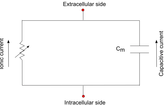
can be modeled as an electric circuit, with a capacitor in parallel to a resistor. The particular form of the ionic current is dictated by the particular model of the membrane under consideration and could be linear or nonlinear in the membrane potential, depending on the absence or presence respectively, of voltage-gated active channels (see Eqs. 1.2 and 1.3). . . 7 1.5 A schematic of the neuronal action potential showing the dierent

(15)

1.6 A schematic of a chemical synapse. An action potential in the presy-naptic axon terminal triggers the entry of calcium ions into the termi-nal, which in turn causes the exocytosis of the neurotransmitter in to the synaptic cleft. The neurotransmitter then triggers excitatory or inhibitory postsynaptic potentials. (Image from Nrets at en.wikipedia, URL: http://en.wikipedia.org/wiki/File:SynapseIllustration2.svg). . 13 1.7 A schematic of a gap junction. Allowing for direct passage of ions in

(16)

1.8 Polarization (induced membrane potential) of a passive cylindrical neuron (radius 2 µm and length 8 µm) in the presence of a uniform

electric eld of strength 1 V/m (steady-state eld is in the positive

z-axis direction i.e. bottom to top in the orientation of the above

gures). The color scheme represents the membrane potential, Vm=

Vi−Ve(in mVs) which is a measure of the charge accumulation on the capacitive membrane (withcmas the per unit area capacitance). The charge density in the bulk regions is zero (see above section 1.4). The results are derived using the nite-element scheme (section 2.5.2) a) Polarization due to the steady-state eld. The neuron end proximate to the positive terminal is hyperpolarised (positive charge outside and negative inside) whereas the neuron end proximate to the negative terminal is depolarised (negative charge outside and positive inside), as expected. b) Polarization due to oscillating eld (100 Hz) with oscillation phase of π. The eld polarity is reversed with respect to

a) and so is the polarization of the neuron. c) Polarization due to oscillating eld (100 Hz) with oscillation phase of π

4. d) Polarization due to oscillating eld (100 Hz) with oscillation phase of 3

(17)

1.9 Current ow in a eld-neuron system with a passive cylindrical neuron (radius 2 µm and length 8 µm) in the presence of a uniform electric

eld of strength 1 V/m (steady-state eld is in the positive z-axis

direction i.e. bottom to top in the orientation of the above gures). The arrows represent the direction and strength of the current density

J in the bulk regions (in A/m2_{). The contours are lines of constant} potential with the color scheme representing the intracellular (left colourbar) and the extracellular (right colourbar) potential (in mVs). The results are derived using the nite-element scheme (section 2.5.2) a) Current ow due to the steady-state eld. The current ows from the positive terminal to the negative one while diverting away from the high resistance membrane. b) Polarization due to oscillating eld (100 Hz) with oscillation phase ofπ. The current direction is reversed

with respect to a). c) Current ow due to oscillating eld (100 Hz) with oscillation phase of π

4. d) Current ow due to oscillating eld (100 Hz) with oscillation phase of 3

(18)

1.10 Two alternative ways of cell stimulation. (a) (Left) Current injection via whole cell patch-clamp: The membrane behaves isopotentially and the cell response is dependent on the membrane conductance and ca-pacitance, not on the extra and intracellular conductivities (Eq. 1.24). (Right) Membrane potential distribution on a spherical neuron of ra-dius 10µm in the presence of an electric eld oriented along thex-axis.

The membrane potential is dependent on the position on the cell as well as the extra and intracellular conductivities (Eq. 1.21). (b) Nor-malized membrane potential responses of a passive current-injected and a passive eld-stimulated spherical neuron (of radius 10 µm) to

sinusoidal stimulation at varying frequencies. The current-injected point-neuron response (Eq. 1.24) falls o at around 10 Hz stimula-tion frequency, whereas the eld-stimulated response (Eq. 1.21) is sustained up to kHz frequencies. Parameter values are as in table 1.1. 24

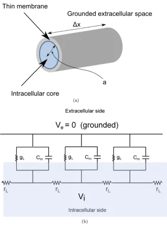
2.1 Schematic of a pyramidal neuron in an electric eld. In a typical ex-perimental setup, an in vitro neuronal slice is placed between parallel eld electrodes, which are used to apply an electric eld. The applied eld is uniform far away from the cell and is in general aligned with the axo-dendritic axis of the neuron. . . 29 2.2 The core conductor model for a dendrite. a) A small section of a

(19)

2.3 Steady-state membrane potential proles for sealed-end cable neurons of various electrotonic lengths (Le =0.5, 1, 2 and 4), in a uniform electric eld oriented along the cable length. Vm is plotted against the distance along the cable x (measured in units of λ), with x only

ranging from 0 to the cable half-length l, due to symmetry.

Elec-trotonically longer cables are more eccentrically polarized than the shorter ones and Vm takes on a linear prole near the center of the cable (x = 0) for all electrotonic lengths. The parameters used to

produce this gure are as given in table 1.1, with the cable radius

a= 2 µm and λ= 447.2 µm. . . 36

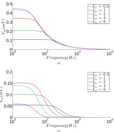
2.4 Electrotonically compact neurons remain responsive to high-frequency electric eld stimulation. a) Frequency response of cable neurons of various electrotonic lengths (box top right) to electric eld stimula-tion, with Vm measured at cable end (x = l). More compact neu-rons (Le = 0.5,1) exhibit a higher drop-o frequency indicating a shorter eective time constant (τcab) for membrane polarization. The

frequency response of all the neurons converges at high frequencies, with the response of the shorter neurons never signicantly exceed-ing that of the longer ones. b) Frequency response of cable neurons with Vm measured at x = ₂l. Frequency selectivity is observed with diering high-frequency asymptotes and the high-frequency response of the compact neurons (Le = 0.5,1) exceeds that of the elongated ones (Le = 4,8). The parameters used to produce these gures are as given in table 1.1, with the cable radius a= 2 µm and λ= 447.2

(20)

2.5 Steady-state Vm plotted against electrotonic length for various frac-tional positions (box top right) along the cable neuron exposed to a uniform eld. The non-monotonic proles indicate that due to the in-creasingly eccentric polarization proles of the longer cable neurons, a shorter neuron will give a larger response for the same o-end frac-tional position, which in turn leads to the high-frequency selectivity for the shorter cable neurons (g. 2.4). The parameters used to pro-duce this gure are as given in table 1.1, with the cable radius a= 2

µm and λ= 447.2 µm. The neurons considered have sealed ends. . . 44

2.6 A dierence in cable-end boundary conditions do not have a signicant impact on the frequency response of the cable neurons. Frequency response for cable neurons of electrotonic lengths Le = 0.5 and 2 for both sealed-end and conducting-end boundary conditions. The responses for the two boundary conditions are virtually superimposed at this resolution. The measurements are performed at x = l. The

parameters used to produce this gure are as given in table 1.1, with the cable radius a= 2 µm and λ= 447.2 µm. . . 48

(21)

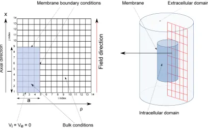
2.8 The nite-dierence grid for a cylindrical neuron exposed to a uniform electric eld, whereais the neuron radius,lis the neuron half-length,

ρ is the radial coordinate,zis the axial coordinate, andVi andVeare the intra and extracellular potentials respectively. Due to the axial symmetry of the cylindrical system only a two-dimensional grid is re-quired. Further symmetry conditions due to the uniform eld require only a quadrant of the eld-cell system to be simulated. Each point on the membrane boundary corresponds to two overlayed points, one in-tracellular and one exin-tracellular, both coupled through the membrane conductance, gL. . . 54

2.9 Steady-state membrane potential distribution on a eld-stimulated cylindrical neuron with a non-conductive membrane (nite-dierence results). The applied eld orientation is along the cylinder axis (x

-axis) a) Membrane potential distribution on the side of the cylinder,

Vx, plotted according to the linear t (Eq. 2.59). As expected, the

neuron is hyperpolarized at the positive eld end, while being depo-larized at the negative end. The cylinder is of size 2_×16 µm (b)

Variation of Vx along the axial direction for dierent cell shapes and sizes (nite-dierence). (c) Normalized variation in the axial direc-tion: Vx/l versus x/l. The plots for the dierent shapes and sizes converge for longer cylinders on to the function Vx =Ex. (d) Mem-brane potential distribution,Vρon the top of the cylinder (x=l= 16

µm), plotted according to the semi-analytical t (Eqs. 2.60 and 2.61). Vρ is axis-symmetric and highest at the center of the cylinder base. (e) Radial distribution of Vρ at x=l, plotted for cylinders of various shapes (numerical simulations). (f) Plots of (Vρ−El)/aVsρ/a eluci-dating the function f ρ_a

. Ana×lneuron corresponds to a cell with

(22)

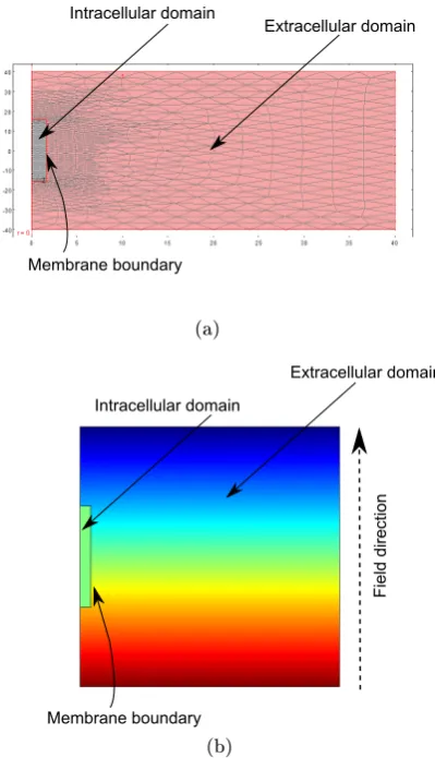
2.10 Results from the nite-element solution method (COMSOL Multi-physics). a) An example mesh for the two-dimensional axial sym-metric problem. The elements are triangular and the mesh resolution increases inside the neuron and around the membrane to take account of the higher eld strengths in those regions, in a computationally e-cient manner. b) A two-dimensional potential plot for the cylindrical neuron in a uniform eld. . . 59 2.11 Membrane potential versus gL comparison between nite-dierence,

nite-element and cable methods for a) 2_×4 µm and b) 2_×16 µm

(compact) cylindrical neurons. The nite-element and nite-dierence results agree very closely but both dier signicantly from the cable results with the dierence greater for the more compact2×4µm

neu-ron. The neurons considered have conducting ends. Vm is measured at the cable end (x = l) and the parameters used to produce these

gures are as given in table 1.1, with the cable radius a= 2 µm and

λ= 447.2µm. . . 61

2.12 Frequency response comparison between nite-dierence, nite-element and cable methods for a)2_×4µm and b)2_×16µm (compact)

cylindri-cal neurons. As in the steady-state case with gL-variation (g. 2.11)

the nite-dierence and nite-element methods agree closely but dif-fer from the cable results, with an increasing error for more compact neurons due to cell-to-eld feedback. The neurons considered have conducting ends. Vm is measured at the cable end (x = l) and the parameters used to produce these gures are as given in table 1.1, with the cable radius a= 2 µm andλ= 447.2 µm. An a×l neuron

(23)

2.13 Comparison between nite-element and and cable methods in ascer-taining the frequency response for cylindrical neurons of electrotonic lengths comparable to λ, in an oscillating electric eld. a) The

fre-quency responses of the Le = 0.5 and 2 neurons show close agree-ment between the eleagree-ment and the cable methods. The nite-element response slightly overtakes that of the cable method for both b) Le= 0.5 and c) Le = 2neurons at high frequencies. The neurons considered have conducting ends. Vm is measured at the cable end (x=l) and the parameters used to produce these gures are as given

in table 1.1, with the cable radiusa= 2µm and λ= 447.2 µm. . . 63

2.14 Comparison between the nite-element and cable methods in ascer-taining the frequency response for compact cylindrical neurons, in an oscillating electric eld. a) The frequency of responses for the l=10

and 20µm neurons dier signicantly between the nite-element and

the cable methods in the low-frequency limit. The log-log plots also reveal that the nite-element response falls slightly below that of the cable method for both b) 10_×10µm and c) 10_×20µm neurons at

high frequencies. The drop-o frequencies are identical for both mod-els. The neurons considered have conducting ends. Vm is measured at the cable end (x = l) and the parameters used to produce these

gures are as given in table 1.1, with the cable radiusa= 10µm and

λ = 1000 µm. An a_×l neuron corresponds to a cell with radius a

and half-length l. . . 64

(24)

3.1 Point-source stimulation of cylindrical neurons (cable neuron (right), and three-dimensional nite-element neuron (left)). Due to the asym-metry imposed by the point-source current, a full three-dimensional model of the neuron has to be considered for the nite-element method. We consider three measurement points on the three-dimensional cylin-der, proximate, middle and far. . . 71 3.2 Steady-state membrane potential proles of cable neurons of various

electrotonic lengths, under point-source stimulation, with the source aligned horizontally with one of the cable-ends (g. 3.1). Vmis plotted against x normalized to the cable length L. Two dierent values of

the source-to-neuron distance are considered, with I = 100 nA. a)

Illustration showing the positioning of the cable neuron with respect to the point source and the point of measurement. b) Plots ford= 0.1λ

and c) d = λ. A biphasic and asymmetric polarization is observed,

with the neutral point located nearer to the stimulation end of the cable. The membrane potential prole becomes more symmetric with smaller L

(25)

3.3 Comparison between the FEM and cable methods for the steady-state membrane potential proles of neurons under point-source stimulation (I = 100 nA) with a)Le = 0.5 andd= 0.1λb) Le = 2and d= 0.1λ c) Le = 0.5 and d=λ and Le = 2and d=λ. The source is aligned horizontally with one of the cable-ends (g. 3.1). Vmis plotted against

xnormalized to the cable lengthL. The cable proles match well with

the middle FEM proles. The dierence between the cable and the proximate / far proles arises due to the radial orientation of the eld at and near x = 0. The neurons considered have sealed ends.

The parameters used to produce these gures are as given in table 1.1, with the cable radius a= 2 µm andλ= 447.2µm. . . 79

3.4 Comparison between the FEM and cable methods for the steady-state membrane potential proles of a compact 10_×10 µm neuron

under point-source stimulation (I = 100 nA). The source is aligned

horizontally with one of the cable-ends (g. 3.1). a) The axial prole of Vm diers greatly between the proximate and far FEM results, and the cable results (∼95% increase inVm for the FEM model). Vm is plotted against x normalized to the cable length L. The neuron

considered has sealed ends. b) Radial variation of Vm across the top of the FEM three-dimensional cylindrical neuron (taking a line from the proximate to the far point), with conducting and sealed ends. The radial eld due to the point-source induces a radially varying membrane potential across the top of the cylinder. The parameters used to produce these gures are as given in table 1.1, with the cable radius a= 10µm andλ= 1000 µm. Ana×l neuron corresponds to

(26)

3.5 Electrotonically compact cable neurons remain responsive to high-frequency electric eld stimulation from a point-source (I = 100 nA

andVmis measured at the cable end proximate to the point-sourcex=

0). Frequency response of neurons of various electrotonic lengths (box

top right) to point-source electric eld stimulation, withVmmeasured at the cable end closest to the source. Like in the uniform eld case (g. 2.4), more compact neurons exhibit a higher drop-o frequency indicating a shorter time constant for membrane polarization. The frequency response of all the neurons converge at high frequencies, with the response of the shorter neurons never signicantly exceeding that of the longer ones. Two dierent values of d: a) 0.1λ and b) λ

are used. The neurons considered have sealed ends. The parameters used to produce these gures are as given in table 1.1, with the cable radius a= 2µm and λ= 447.2 µm. . . 82

3.6 Comparison between cable neurons under uniform and point-source eld stimulation withd= 0.1λ(I = 100nA andVmis measured at the cable end, x= 0). Neurons with two diering sizes: a) Le= 1 (with

a= 2µm andλ= 447.2µm) and b)10_×10µm (witha= 10µm and λ = 1000 µm) are considered. Both point and uniform stimulation

produce the same frequency drop-os. The neurons considered have sealed ends. The parameters used to produce these gures are as given in table 1.1. Ana_×l neuron corresponds to a cell with radiusaand

(27)

3.7 Comparison between nite-element and cable methods in ascertaining the frequency response for cylindrical neurons of electrotonic length

Le = 1, in an oscillating point-source electric eld (I = 100 nA and

Vm is measured at the cable end x= 0). The middle point for the FEM model matches well with the cable model for both a) d= 0.1λ

and b) d= λ. An additional high-frequency plateau is observed for

the FEM models. The measurement is performed at the cable end proximate to the source. The neurons considered have sealed ends. The parameters used to produce these gures are as given in table 1.1, with the cable radius a= 2 µm andλ= 447.2µm. . . 84

3.8 Comparison between nite-element and and cable methods in ascer-taining the frequency response for a compact cylindrical neuron of size

10_×10 µm , in an oscillating point-source electric eld (I = 100 nA

and the measurement is performed at the cable end proximate to the source x = 0). The FEM results for the proximate and far points

dier greatly from the cable model for both a)d= 0.1λand b)d=λ.

The dierence is caused by the radial prole of the extracellular eld for small L

d ratios. The neurons considered have sealed ends. The parameters used to produce these gures are as given in table 1.1, with the cable radius a= 10µm and λ= 1000µm. An a_×lneuron

(28)

3.9 The passive resonance is observed for o-end measurement of ca-ble neurons under point stimulation (with Vm measured at x = L₄). Frequency response of cable neurons of various electrotonic lengths (box top right) with a) d= 0.1λand b) d=λ. Frequency selectivity

is observed with diering frequency asymptotes and the high-frequency response of the compact neurons exceeds that of the elon-gated ones. Additionally strong and broad resonances are observed for Le=1, 2 and 4 in thed= 0.1λcase. The neurons considered have sealed ends and the parameters used to produce these gures are as given in table 1.1, with the cable radius a= 2 µm andλ= 447.2 µm. 87

3.10 Frequency response of cable neurons (of various electrotonic lengths (box top right)) under point stimulation, with Vm measured at the center x = L

2, with a) d = 0.1λ and b) d = λ. Frequency selec-tivity is observed with diering high-frequency asymptotes and the high-frequency response of the compact neurons exceeds that of the elongated ones. No resonance is observed. The neurons considered have sealed ends and the parameters used to produce these gures are as given in table 1.1, with the cable radiusa= 2µm andλ= 447.2µm. 88

3.11 Frequency response of cable neurons of various electrotonic lengths (box top right) under point stimulation, withVm measured atx= 3₄L, with a)d= 0.1λand b)d=λ. Frequency selectivity is observed with

(29)

3.12 Frequency response of cable neurons of various electrotonic lengths (box top right) under point stimulation, with Vm measured atx=L, with a)d= 0.1λand b)d=λ. Frequency selectivity is observed with

diering high-frequency asymptotes and the high-frequency response of the compact neurons exceeds that of the elongated ones. No reso-nance is observed. The neurons considered have sealed ends and the parameters used to produce these gures are as given in table 1.1, with the cable radius a= 2 µm and λ= 447.2 µm. . . 90

3.13 Development of the localized resonance through the length of the cable neuron from x= 0.1L to x= 0.5L. The neuron under consideration

is of sizeLe= 1and has sealed ends. The parameters used to produce these gures are as given in table 1.1, with the cable radiusa= 2 µm

and λ= 447.2µm. . . 92

3.14 Passive resonance is observed for the three-dimensional FEM models as well as for the cable models (measurement performed at x= 0.25L

with horizontal electrode-neuron distance d = 0.1λ). The neuron

under consideration is of sizeLe = 1. The high-frequency plateau for the FEM case is observed as in the cases where the measurements are performed at x =l above (g. 3.7). The neuron has sealed ends and

(30)

3.15 The passive resonance is observed for o-end point stimulation of cable neurons. Frequency response of cable neurons of various elec-trotonic lengths (box top right). The horizontal electrode-cell distance isd= 0.1λa) Point-source is placed next to the vertical center of the

neuron and the measurement is performed at x = 0. No resonance

is observed. b) Point-source is placed next to the vertical center of the neuron and the measurement is performed at x= 0.25L. No

res-onance is observed. c) Point-source is placed a quarter of the way up the length of the neuron (x= L

4) and the measurement is performed at x = 0. Strong and broad resonances are observed. The neurons

considered have sealed ends and the parameters used to produce these gures are as given in table 1.1, with the cable radius a= 2 µm and

λ= 447.2µm. . . 94

3.16 The passive resonance is observed for point stimulation of cable neurons with conductive ends (horizontal electrode-cell distance is

d = 0.1λ). Frequency response of cable neurons of various

electro-tonic lengths (box top right). a) Point-source is placed at x= 0 and

the measurement is performed at x = L

4. b) Point-source is placed at x = L

(31)

3.17 The dierent features of the frequency prole for the point-stimulated FEM cylindrical neuron. The FEM and cable plots are as in g. 3.7a for cylindrical neurons of electrotonic length Le= 1, in an oscillating point-source electric eld (I = 100 nA, d = 0.1λ and Vm is mea-sured at the cable end, x =l). In agreement with the cable plot, all

three FEM proles exhibit the low frequency plateau and the same frequency drop-o. In contrast with the cable plot, the proximate and far point proles also exhibit a high frequency plateau. This high frequency plateau is also seen in measurements with the passive resonance (g. 3.14). . . 98

4.1 Electric circuit models of active membranes. a) Representation of non-linearized two-component system with one type of voltage-gated channel. b) The LRC Circuit representing the the linearised form of the two-component system in a). The inductance,L= τn

κ and the con-ductances are given by κ=gn(Vm∗−En)dn_dV∞_m|V∗

m and gT =gL+gnn

∗_.

(32)

4.2 Frequency response for eld-stimulated neurons of various shapes (Spher-ical, nite-element and cable results) with quasi-active membranes in a uniform oscillating eld. a) Comparison between the current-injected neuron and the eld-stimulated spherical neuron of radius 10µm

(ana-lytical solutions in Eqs. 4.11 and 4.12 respectively). The subthreshold resonance is clearly evident in the current-injected case whereas it is eliminated in the eld-stimulated spherical neuron case. b-d) Com-parison between eld-stimulated cylindrical neurons of electrotonic lengths Le = 0.5, 1 and 2, respectively, with the measurement per-formed at the cable end (x=l). The resonance disappears for neurons

with low electrotonic lengths but is recovered for elongated neurons. Both the FEM and cable results agree well for the given neuron sizes. The cable neurons under consideration have sealed ends. The param-eters used to produce these gures are as given in table 4.1, with the cable radius a= 2 µm andλ= 447.2 µm. . . 105

4.3 The passive resonance in the Hodgkin Huxley Neuron. a) The res-onance prole for a passive cable neuron of size Le = 1, under point stimulation (I = 100 nA) at x = 0 and measured at x = 0.25L.

The horizontal electrode-cell distance is d = 0.1λ. The parameters

(33)

4.4 A point-stimulated, nite-element spiking neuron of size Le = 1 and

I = 100 nA (the stimulation and measurement points are as in g.

4.3). The rising amplitude due to the resonance can be seen going from a) 5 Hz to b) 10 Hz to c) 100 Hz with the 100 Hz neuron ring.

I = 2000 nA for all the models. The parameters are as given in table

4.2. The neurons considered have sealed ends with the cable radius

a= 2 µm and λ= 447.2 µm. . . 112

4.5 The semi-innite neuronal array a) A schematic of the 3-dimensional eld-stimulated neuronal array, simulated using the nite-element method. The periodic boundary conditions along the eld-perpendicular axes simulate an eectively innite number of neurons along these direc-tions. The cumulative height of cells is maintained at approximately 100 µm above and below the central observed cell. b) Normalized

steady-state membrane potential distribution, Vx/x for a 4×4×4 and 4_×4_×32µm passive array-embedded neuron exposed to a

non-oscillating electric eld oriented along the x-axis. The eld-coupling

for the array-embedded neuron is much greater than for the isolated case, with the magnitude of the induced membrane potential approx-imately twice that for an isolated neuron. The parameters used to produce b) are as given in table 1.1. Anw_×d_×lneuron corresponds

(34)

4.6 Frequency response for a passive array-embedded neuron exposed to an oscillating electric eld (the measurement is performed at the top-right corner of the central neuron). The array-embedded cell is com-pared with the monolayer-embedded and the isolated cases for cell sizes of a) 4_×4_×4µm and b)4_×4_×32µm. The drop-o frequency

decreases going from the isolated to the full array-embedded neuron, with the cells in the eld-perpendicular plane primarily contributing to the change as demonstrated by the monolayer case. The eect of cell elongation on the drop-o frequency is still apparent with the array-embedded neuron. The parameters used to produce these g-ures are as given in table 1.1. An w_×d_×l neuron corresponds to a

cell with width w, depthdand half-lengthl. . . 116

4.7 Frequency response for a quasi-active eld-stimulated neuron embed-ded in array and exposed to an oscillating electric eld (the measure-ment is performed at the top-right corner of the central neuron). The array-embedded cell is compared with the monolayer-embedded and the isolated cases for cell sizes of a)4_×4_×256µm and b)4_×4_×512

µm. Analogous to the isolated neuron case, the resonance reappears

for the longer neuron. Additionally the resonance amplitude increases going from the isolated case to the monolayer-embedded or the eld-embedded cases. The parameters used to produce these gures are as given in table 4.1. An w_×d_×l neuron corresponds to a cell with

(35)

Declarations

(36)

Chapter 1

Introduction

1.1 The neuron as a computational engine

The neuron is the fundamental biological component of the nervous system, the func-tionality of which provides for the information processing capability of the complex neuronal networks in the brain. Thus understanding the full functional capabilities of the single neuron is crucial towards gaining insight in to the long sought after questions about how cognition and sentience are mediated by the interconnected networks of some 86 billion neurons in the human brain.

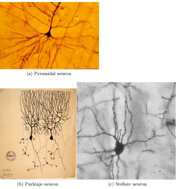
Neurons are widely dierentiated in terms of their size and shape, with cell bodies ranging from 5-120µm and shapes ranging from the pyramidal to the stellate

(37)

(a) Pyramidal neuron

[image:37.595.125.469.109.478.2]

(b) Purkinje neuron (c) Stellate neuron

(38)

The nerve cell can thus be thought of as the multiplex neuron as proposed by Waxman [1], where information processing occurs at distinct hierarchical levels of the cell; rstly in the dendrites through the spatiotemporal summation of exci-tatory and inhibitory synaptic inputs, secondly at the soma and the axon initial segment which can receive further synaptic inputs [25] and thirdly in the axonal tree and the end terminals with further synaptic inputs [6]. Thus the neuron is envisaged as analogous to a microelectronic chip rather than a gate [1, 7], a de-scription far removed from the point-neuron view of the nerve cell as employed by McCulloch and Pitts in their 1943 paper on neural computation [8], consisting of a threshold computing soma receiving linear preprocessed synaptic inputs. This description highlights the substantial information processing power available to the nervous system even at a single cell level. With the discovery of active channels in the dendrites, facilitating forward and back propagating action potentials [912], and axon transmission delays and branch point failures facilitated by axonal morphology and channel biophysics [13], the role of the dendrites and axons has been extended beyond the simple transmission of input and output signals. In short, investigators are nding the neural chip to be more and more complex [1316].

(39)

(40)

in the presence of extracellular electric elds. Finally, we highlight a discrepancy in the experimental literature considering eld-cell interactions, before going on to jus-tify the need for modeling extracellular electric eld interactions within the nervous system.

1.2 The membrane and the membrane potential

The biological membrane is a lipid bilayer embedded with functional protein com-plexes (g. 1.3), in general impermeable to most charged molecules and thus acts like a capacitor in separating charge on either side. The membrane allows current ow through embedded ion channels which provide for selective ion permeabilities. The essential variable which denes single neuron function is the membrane poten-tial, a dierence in potential which exists across the plasma membrane of all cells. For neurons at rest, this potential dierence arises because of the dierence in ionic concentrations (maintained by active ionic pumps) between the inside and outside of the cells with the membrane having dierent permeabilities for dierent ions. The membrane thus can be modeled by a simple electric circuit with a capacitor acting in parallel to a resistor (g. 1.4). This model implies a transmembrane current density

J =cm

∂

∂tVm+Iion(Vm) (1.1)

wherecm is the membrane capacitance per unit area,Vm is the membrane potential (inside minus outside) andtis the time. The rst term on the right hand side of Eq.

1.1 is the capacitive current density while Iion is the ionic current density through the channels. For subthreshold conditions when only the passive leak channels are open,Iion is commonly modeled as a linear function of the membrane potential [17]

(41)

Figure 1.3: A schematic of the biological membrane. The membrane consists of a lipid bilayer with embedded proteins. Acting as a selective barrier, separating the intracellular cytoplasm from the extracellular space, the membrane is impermeable to most charged molecules. The protein ion channels are selectively permeable across the membrane and can be leak, voltage-gated or ligand-gated (Image from Mariana Ruiz Villarreal at en.wikipedia, URL: http://en.wikipedia.org/wiki/File:Scheme_ facilitated_diusion_in_cell_membrane-en.svg).

where gL = Pgi is the leak conductance per unit area and EL =

P

giEi

gL is the resting membrane potential, withgi and Ei as the membrane conductance per unit area and the Nernst potential for theith ion, respectively.

(42)

Extracellular side

Intracellular side

Ioni

c

cu

rr

en

t

Ca

pa

citive

cu

rr

en

t

[image:42.595.124.459.104.319.2]

Cm

Figure 1.4: The electric circuit model of the neuronal membrane. The membrane can be modeled as an electric circuit, with a capacitor in parallel to a resistor. The particular form of the ionic current is dictated by the particular model of the membrane under consideration and could be linear or nonlinear in the membrane potential, depending on the absence or presence respectively, of voltage-gated active channels (see Eqs. 1.2 and 1.3).

these channels into the transmembrane current densityJ, we obtain

J =cm_∂t∂Vm+gL(Vm−EL) +gKn4(Vm−EK) +gN am3h(Vm−EN a) (1.3)

wheregK andgN aare the maximal conductances per unit area for the potassium and sodium ions respectively (they are the conductances per unit area if all the channels of the respective type are open),EK andEN aare the potassium and sodium reversal potentials respectively, andn, m and h are the gating variables described by their

respective rate equations.

Equation 1.3 represents the membrane currents as described by the Hodgkin Huxley model [18] and is an example of a conductance-based description of the membrane potential dynamics, where the current density through a particular ion channel is given by the product of the conductance per unit area and the driving force

(43)

hand side of equation 1.3 represent the capacitive and the leak currents, respectively as stated earlier. The last two terms in equation 1.3 describe the currents through the potassium and the sodium channels respectively, with voltage-gated conductances which are given by the product of the maximal conductances and the probabilities that the respective channel is open (given by the products of the gating variables). The voltage dependence arises becausen,mand h are dependent onVm and hence

t. For the persistent (noninactivating) potassium current density, the conductance

is given by gKn4, where n4 is the probability that the channel will be in an open state. The exponent of four for the gating variable n is essentially a functional

value, being also consistent with the four subunits comprising the potassium channel, acting independently (with the probability of a single subunit opening to ben). The

potassium conductance being noninactivating, only requires an activation gating variable (n), which increases with increasing depolarization.

For the transient sodium current density, the conductance is given bygN am3h, where now the probability of channel opening is given by the product of two gat-ing variables m3_h_{, to account for the transient nature of the conductance. Here}

m and h represent the activation and the inactivation gates of the sodium channel

respectively. With increasing depolarization, m increases and activates the channel

whereashdecreases and eventually inactivates the channel. It should be noted that

the channel opening probabilities (n4 _and _m3_h_{) represent the fractions of channels} (for potassium and sodium ions respectively) which are open at a particular time and arise from a deterministic description of the channel dynamics (justied by the large numbers of stochastically uctuating individual channels). The dynamics of the gating variables are described by equations of the form

dj

dt =αj(Vm)(1−j)−βj(Vm)j (1.4)

(44)

is the product of the closed probability and the opening rate and thus represents the probability that the subunit opens in a short time interval. Similarly, the rst term on the right hand side of Eq. 1.4 is the product of the open probability and the closing rate and thus represents the probability that the subunit closes in a short time interval. Thus the dierence of the two terms gives the rate of change of the open probability j. The rate functions are obtained by tting experimental data,

but the general form can be derived using thermodynamic arguments (see chapter 5 of [84]). The particular expressions for the rate functions used in this thesis, are given in section 4.2, where we model active neurons in the presence of extracellular electric elds.

The action potential is propagated along the axonal ber due to the excitation of downstream sodium channels through extracellular and intracellular local circuit currents which ow passively between the active zone and the oncoming dormant part of the axonal ber.

Traditional point-neuron models assume the transmembrane current and hence

Vm to be spatially independent, leaving a one-dimensional system of dierential equations to be solved. The development of linear cable theory in the late 1950s by Rall [19] allowed modelers to treat dendrites as one-dimensional core conductor cables surrounded by a passive membrane. In the majority of these modeling ap-proaches, assumptions are made which a priori exclude the possibility of realistic extracellular interaction. In the rst instance, the extracellular potential is assumed to be grounded at zero, implying that no injection of current occurs in the extra-cellular space, either from other neurons or an articial source. Secondly, when an extracellular potential is imposed, it is decoupled from the activity of the neuron itself.

(45)

(46)

allel nerve bers via extracellular ephaptic coupling were demonstrated as far back as 1940 [20,21]; Katz and Schmitt being the rst to do so using the crab limb nerve model [20]. Axo-axonal interactions have been proposed to occur in situations where the myelin sheath is compromised or the nerves are brought into unphysiological proximity, such as in multiple sclerosis or in crushed nerves [22]. In such a situation an action potential in one axon can change the excitability of or even cause an action potential in the neighboring axons through local extracellular currents. This type of ephaptic interaction is also hypothesized to occur in physiological conditions where the axons are tightly packed, increasing the extracellular resistance, such as in the mammalian olfactory nerve fascicles containing unmyelinated axons [23,24]. Another type of ephaptic communication is via the modulation of the spike threshold, where the extracellular potential around an axon hillock is modied through the action of other neurons. This type of communication, providing for fast local inhibition of the spike initiation zone has been shown to occur within specialized structures around the teleost Mauthner and the mammalian cerebellar Purkinje cells [25,26]; to date the only known cases of ephaptic coupling in non-pathological systems without articial electrical stimulation.

(47)

1.3 Synapses: How neurons communicate

For a neuron the input for the neuronal computations typically comes through the chemical synapses; highly specialized structures which provide for the main lines of communication between neurons within the nervous system (g. 1.6). Form-ing between the presynaptic axon terminal and a part of the postsynaptic neuron, chemical synapses can be axodendritic, axosomatic or axoaxonal and number around 240 trillion in the cerebral cortex [83]. Communication through the synapse occurs when an action potential arrives at a presynaptic terminal causing the activation of voltage-gated calcium channels leading to a rise in the intracellular calcium concen-tration within the terminal. This triggers the probabilistic release and diusion of neurotransmitters (packaged in synaptic vesicles within the terminal) into the synap-tic cleft due to calcium-dependent exocytosis. The neurotransmitter then binds to specic receptors on the postsynaptic membrane causing specic changes in ionic permeabilities leading to depolarization and excitation or hyperpolarization and in-hibition of the postsynaptic cell through postsynaptic potentials.

(48)

Figure 1.6: A schematic of a chemical synapse. An action potential in the presynaptic axon terminal triggers the entry of calcium ions into the terminal, which in turn causes the exocytosis of the neurotransmitter in to the synaptic cleft. The neurotransmitter then triggers excitatory or in-hibitory postsynaptic potentials. (Image from Nrets at en.wikipedia, URL: http://en.wikipedia.org/wiki/File:SynapseIllustration2.svg).

communication within the nervous system. Electrical synapses or gap junctions mediate electrical transmission between adjacent neurons. Constructed from con-nexons, arrays of paired hexameric ion channels, gap junctions (g. 1.7) allow small molecules to pass between the connected neurons, in turn allowing potentials (in-cluding action potentials) to spread between the cells at very short time scales. Gap junctions are known to play an important role in fast neuronal synchronization [45].

1.4 General equations - coupling the membrane to

elec-tric elds

(49)

(50)

domains is described by the simplied version of the Nernst-Planck equation

J=₋σ_∇V (1.5)

whereσis the conductivity andV is the potential. Application of charge conservation

gives the continuity equation

∂ρ

∂t +∇ ·J= 0 (1.6)

whereρis the charge density. Combining Eqs. 1.5 and 1.6 above gives

∂ρ ∂t =σ∇

2_V _(1.7)

Now utilizing the dierential form of Gauss' Law describing how the charge density inuences the electric eld

∇ ·E= ρ (1.8)

∇2_V ₌₋ρ

(1.9)

where we have used the denition of the electric potentialE =−∇V to obtain Eq.

1.9, withE as the electric eld andas the permittivity. Substituting from Eq. 1.9

in to Eq. 1.7 we get

∂ρ ∂t =−

σ

ρ (1.10)

Thus we see that the charge density in the bulk domains goes to zero with a time constant

σ. For our purely resistive model of the extracellular and intracellular domains we have

(51)

the system comes from the oscillating electric eld, and the membrane capacitance and voltage-gated conductances. This assumption is justied as the typical value of the time constant

σ is ~ 3 µs in tissue compared to the typical value of 10 ms for the membrane time constant. Withρ = ∂ρ_∂t = 0 in the bulk domains, the intra and

extracellular potentialsVi and Ve respectively, satisfy Laplace's equation [46,47]

∇2Vi=∇2Ve= 0 (1.11)

Thus in our theoretical framework we do not need to model the ionic charge distri-bution as is done in the Poisson-Boltzmann equation, and similarly considerations such as Debye screening can be ignored. To give the reader an intuitive picture of the charge distribution and current ow in a cell-eld system, we have plotted the membrane potentialVm(g. 1.8) and the current density (g. 1.9) for a eld-neuron system, with a steady-state and an oscillating eld (at dierent phases). Note the reversal of the current ow and the neuron polarization which occurs when the eld reverses orientation (at phases of π and 3₄π for a cosine oscillation).

The boundary conditions far away from the cell are determined by assuming that the cell is small compared to the extracellular region and is located away from the external boundaries, giving the extracellular potential

Ve(r, t) =E·r |r| → ∞ (1.12) wherer is the position where the potential is being calculated with respect to the

origin and E is the uniform applied electric eld. We assume that the potential

across the membrane is discontinuous, with Vm as the dierence between the intra and extracellular potentials. The transmembrane current density,J is given by

J =₋n_·(σi∇Vi) =cm

∂

(52)

wheren is a unit normal pointing outward from the membrane and σi and σe are the intra and extracellular conductivities respectively. Eq. 1.13 ensures that J is

continuous across the membrane and relates it to the membrane potential, resulting from the membrane and the bulk media properties.

1.5 Deriving the time-dependent solution from the

steady-state solution

Using the general boundary-value problem above (Eqs. 1.11-1.13), we can derive a simple recipe for converting the steady-state solution to the oscillatory time-dependent one, where the stimulating uniform external eld is given byEo+ ˆEeiωt, wherei=√−1andωis angular frequency of the sinusoidal eld oscillations in time.

If we assume the ansatz

Ve(r, t) =Veo(r) + ˆAe(r)eiωt r≥a (1.14)

Vi(r, t) =Vio(r) + ˆAi(r)eiωt r≤a (1.15) for the time-dependent oscillatory solution, applying the bulk Laplace equation (Eq. 1.11) to the above solution form, results in the Laplacians of Vo

e, Vio, Aˆe and Aˆi equaling zero independently. So the initial general forms forVo

e and Aˆe have to be identical to the initial general form of the steady-state solutionVe(r), and the initial general form for Vo

i and Aˆi have to be identical to the initial general form of the steady-state solutionVi(r).

A simple application of the far away boundary condition (Eq. 1.12) and the continuity boundary condition from Eq. 1.13 (i.e. −n_·(σi∇Vi) = −n·(σe∇Ve)), and matching the oscillatory and non-oscillatory components across equations, shows that the constraints onVo

(53)

(a) (b)

(c) (d)

Figure 1.8: Polarization (induced membrane potential) of a passive cylindrical neu-ron (radius 2 µm and length 8 µm) in the presence of a uniform electric eld of

strength1 V/m (steady-state eld is in the positive z-axis direction i.e. bottom to

top in the orientation of the above gures). The color scheme represents the mem-brane potential,Vm =Vi−Ve(in mVs) which is a measure of the charge accumulation on the capacitive membrane (withcm as the per unit area capacitance). The charge density in the bulk regions is zero (see above section 1.4). The results are derived using the nite-element scheme (section 2.5.2) a) Polarization due to the steady-state eld. The neuron end proximate to the positive terminal is hyperpolarised (positive charge outside and negative inside) whereas the neuron end proximate to the negative terminal is depolarised (negative charge outside and positive inside), as expected. b) Polarization due to oscillating eld (100 Hz) with oscillation phase of

π. The eld polarity is reversed with respect to a) and so is the polarization of the

neuron. c) Polarization due to oscillating eld (100 Hz) with oscillation phase of π 4. d) Polarization due to oscillating eld (100 Hz) with oscillation phase of 3

(54)

(a) (b)

[image:54.595.130.521.120.556.2]

(c) (d)

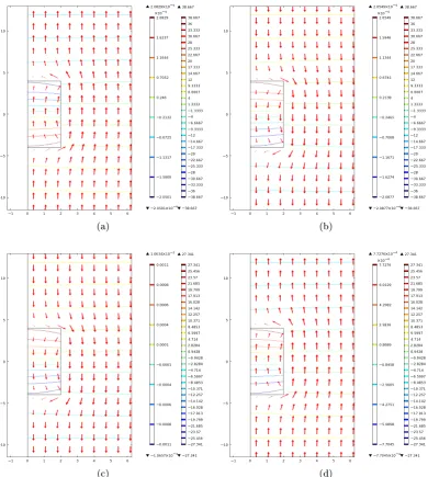
Figure 1.9: Current ow in a eld-neuron system with a passive cylindrical neuron (radius 2µm and length 8µm) in the presence of a uniform electric eld of strength 1V/m (steady-state eld is in the positivez-axis direction i.e. bottom to top in the

orientation of the above gures). The arrows represent the direction and strength of the current density J in the bulk regions (in A/m2_{). The contours are lines of} con-stant potential with the color scheme representing the intracellular (left colourbar) and the extracellular (right colourbar) potential (in mVs). The results are derived using the nite-element scheme (section 2.5.2) a) Current ow due to the steady-state eld. The current ows from the positive terminal to the negative one while diverting away from the high resistance membrane. b) Polarization due to oscillat-ing eld (100 Hz) with oscillation phase ofπ. The current direction is reversed with

(55)

Finally, applying the membrane boundary condition in Eq. 1.13, withIion =

gL(Vi−Ve−EL), we obtain

−σenˆ· ∇(Veo+ ˆAeeiωt) =gL

V_io−V_eo+Aˆi−Aˆe

eiωt−EL

(1.16)

+iωcm

ˆ Ai−Aˆe

eiωt r =a

Matching the non-oscillatory coecients, we obtain

−σeˆn· ∇Veo=gL(Vio−Veo−EL) r=a (1.17) This again implies the identical constraint as that imposed on the steady-state solu-tion by this boundary condisolu-tion. So we can conclude that the solusolu-tions for Vo

e and

Vo

i will be identical to the steady-state solutions with E replaced by Eo. Matching the oscillatory components, we obtain

−σeˆn· ∇Aˆe= (gL+iωcm)

ˆ Ai−Aˆe

r=a (1.18)

−σeˆn· ∇Ae= ˆgL

ˆ Ai−Aˆe

r=a (1.19)

wheregˆL = gL+iωcm. Here we see that the form of the constraint is exactly the same as that for the steady-state case, with the exception of gL → gˆL as well as the absence ofEL. Therefore we conclude that the the solutions forAˆe andAˆi will be identical to the respective steady-state solutions, withE replaced byEˆ, withgL replaced bygˆL and EL= 0.

1.6 Analytical modeling of eld eects on single neurons

- a discrepancy between theory and experiment

(56)

steady-state and dynamic eld interactions with neuronal structures of varying geometries and biophysically detailed membrane properties is needed. Specically, a knowledge of the induced membrane potentialVm, in response to a steady and oscillating electric

eld is a crucial rst step for probing this interaction. The analytical approach to solving this problem for a passive spherical cell exposed to a uniform electric eld was developed by Schwan [46, 47], which involves solving Laplace's potential equation over a domain consisting of highly polarizable intra and extracellular regions with conductivitiesσiand σerespectively, and a thin passive conductive membrane, yielding the expressions (as derived by Grosse and Schwan [47])

Vm =

3/2Eacosθ 1 +agL

1 σi +

1 2σe

static eld (1.20)

ˆ Vm =

3/2 ˆEacosθ 1 +a(gL+iωcm)

1 σi +

1 2σe

sinusoidally varying eld (1.21)

where E and Eˆ are the magnitudes of the static and sinusoidally varying electric

elds respectively,ais the cell radius, θis the polar angle measured from the center

of the cell with respect to the direction of the eld andω is angular frequency of the

oscillating eld (for a detailed derivation, see appendix D). In the physiological range (table 1.1), the expressionagL(_σ1_i+₂_σ1_e)1and thus Eq. 1.20 can be approximated by the original version of the Schwan equation [48]

Vm =

3

2Eacosθ (1.22)

(57)

to a uniform and oscillating electric eld. The resultant equations were simplied by Maswiwat [53,54] avoiding complex expressions for the depolarizing factors used in the original derivation.

It is interesting to contrast Eq. 1.21 with the expression forVm for a passive cell stimulated with direct current injection from an electrode, Iapp = ˆIappeiωt via whole-cell patch clamp (g. 1.10a). The resulting dierential equation is given by

cm

∂

∂tVm =gL(EL−Vm) +Iapp (1.23)

The oscillatory solution to the above equation is given by

ˆ Vm =

ˆ Iapp

gL+iωcm (1.24)

It is important to note that due to the large size of the electrode relative to the cell and the consequent uniform polarization, Eq. 1.24 is not spatially dependent. Both systems exhibit two regimes of behaviour. Firstly, the cell remains responsive up to the frequency given by the reciprocal of the respective time constant. Secondly, above this frequency the response starts to diminish with increasing frequency. The dierent time constants are characteristic of the time it takes for the cell to polarize in response to the stimulation. For the direct current injection case, the time constant is solely dependent on the membrane properties of the cell and is given byτm=cm/gL, which for physiological parameter values (table 1.1) is around 10 ms. In the case of a eld-stimulated spherical cell, the eective membrane time constant, now dependent on the cell radius and the intra and extracellular conductivities, is given by

τsph=

cm 2σe a1+2σe

σi +gL

= τm

1 + 2σe gLa

1+2σe

σi

(1.25)

For a 10µm cell and physiological values for the membrane and bulk media properties

(58)

spherical cell remains responsive to eld stimulation of∼100kHz frequency, whereas

in the current injection case the response drops o after about 10 Hz (g. 1.10b). This high-frequency response, predicted by the time-dependent version of the Schwan equation [46, 47] has been observed in vitro for eld stimulated spherical Murine myeloma cells [55]. The same response however, had not been seen in experiments with pyramidal cells in rat hippocampal slices exposed to AC electric elds [36]. These cells are not compact but are highly elongated, suggesting that the shape of the cell may be important in determining its frequency response to an oscillating electric eld.

Table 1.1: Parameters for the passive membrane. We have articially set the resting membrane potential EL to be zero for ease of notation. We note that for passive models, setting the resting potential to zero only osets the resulting membrane potential byEL and does not inuence the membrane dynamics.

Parameter Denotation value

Extracellular medium conductivity σe 0.2µSµm−1 Cytoplasmic conductivity σi 0.2µSµm−1 Membrane leak conductance gL 1×10−6 µSµm−2

Membrane capacitance cm 1×10−5 nFµm−2 Assumed leak reversal potential EL 0 mV

Membrane time constant τm 10 ms

1.7 The need for modeling electric eld eects

(59)

(a)

100−1 101 103 105 107 109 0.5

1

F requency(Hz)

N or m a li z ed a m p li tu d e ( m V ) Current injected F ield stimulated

(b)

Figure 1.10: Two alternative ways of cell stimulation. (a) (Left) Current injection via whole cell patch-clamp: The membrane behaves isopotentially and the cell response is dependent on the membrane conductance and capacitance, not on the extra and intracellular conductivities (Eq. 1.24). (Right) Membrane potential distribution on a spherical neuron of radius 10µm in the presence of an electric eld oriented along

thex-axis. The membrane potential is dependent on the position on the cell as well

as the extra and intracellular conductivities (Eq. 1.21). (b) Normalized membrane potential responses of a passive current-injected and a passive eld-stimulated spher-ical neuron (of radius10 µm) to sinusoidal stimulation at varying frequencies. The

current-injected point-neuron response (Eq. 1.24) falls o at around 10 Hz stimula-tion frequency, whereas the eld-stimulated response (Eq. 1.21) is sustained up to kHz frequencies. Parameter values are as in table 1.1.

not always fully taken into account as in the example of cable theory [19,56,57]. Our aim is to build three-dimensional, two-way coupled models which fully incorporate the feedback, which in reality exists between the neuron and the extracellular eld as demonstrated recently by Frohlich and McCormick [59]. This will provide for realistic modeling of eld eects on the nervous system in pathological, physiological and clinical contexts. The models will require a synthesis of two dierent modeling approaches used in two dierent elds; rst the nonlinear time-varying behaviour of the membrane characterized by the Hodgkin Huxley equations [18] used exten-sively in theoretical and computational neuroscience, secondly the volume conductor behaviour in the bulk media found by the solution of Maxwell's equations.

(60)

ship between the neuron shape and its response at varying eld frequencies. We use the nite-dierence and nite-element methods for solving the analytically awkward problem of a nite cylinder in an oscillating electric eld. We compare these results with those obtained through the extracellular cable equation and delineate the re-lationship between cellular shape, orientation and susceptibility to high-frequency electric elds. In particular we nd that the neurons stimulated by extracellular elds exhibit an eective membrane time constant dependent on their electrotonic length and thus resolve the discrepancy in the literature, highlighted in section 1.6. In the context of cable theory (see section 2.2), the electrotonic length, Le is the physical length of the neurite under consideration (L), measured in units of the

electrotonic length constant

λ=

r

a

2rLgL (1.26)

where a is the radius of the cable, rL is the intracellular resistivity and gL is the membrane leak conductance per unit area as before. λrepresents the distance over

which a current input in to the dendrite will spread and hence inuence the mem-brane potential. Physically, a larger a and a smaller rL would impose a smaller resistance to current spread (leading to a largerλ), whereas a larger gL would lead to more current escaping in to the extracellular space (and hence a smallerλ).

In chapter 3 we investigate the behaviour of the passive cylindrical cell un-der point-source stimulation. Deriving the cable results using Green's functions, we compare them against the results obtained through our nite-element model. Due to the breaking of the axial symmetry by the non-uniform point-source eld, a three-dimensional nite-element model is constructed. Both modeling methodologies reveal a novel form of localized frequency preference by the entirely passive neurons, the magnitude and frequency of which is dependent on the cell geometry and the distance between the neuron and the point-source. To our knowledge this passive resonance has not been reported in the literature before.

(61)

of a quasi-active membrane into our eld-neuron system known to lead to reso-nance at a characteristic stimulation frequency, manifesting itself as a peak in the induced voltage oscillations, when stimulated by current injection via whole-cell patch clamp [60,61]. This phenomenon, found in many parts of the central nervous system, including in neocortical neurons [6265] as well as hippocampal pyramidal cells [66,67] and interneurons [67], arises from an interplay between the passive and active neuronal properties. In particular, resonance requires voltage-gated currents, which slowly oppose membrane potential changes [60]. Here we apply the linearized quasi-active membrane model to the spherical and the cylindrical eld-neuron sys-tems, elucidating the relationship between the neuronal shape and its subthreshold resonance in the presence of an oscillating electric eld.

We then go on to construct a fully active eld-neuron nite-element model incorporating Hodgkin Huxley type channels into the membrane. A signicant and novel step towards modeling eld-neuron systems with full two-way feedback between the neuron and the eld, we use the spiking model to demonstrate that the passive resonance and high-frequency response of the passive neurons under point-source stimulation translates to the fully active neuron case.

Lastly, we go further and simulate the frequency response of passive neurons embedded in semi-innite arrays and exposed to extracellular elds, validating the results obtained for the case of isolated neurons.

(62)

(63)

Chapter 2

Modeling passive cylindrical

neurons in uniform electric elds

2.1 Introduction

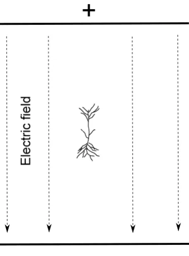
In section 1.6 we presented an apparent discrepancy in the literature with regards to the high-frequency response of cells exposed to oscillating electric elds. The analytical Schwan equation [46, 47] for spherical cells, predicts a membrane poten-tial response to elds oscillating at frequencies even in the kHz range (g. 1.10a). These results were experimentally veried by Marszalek et al [55] with experiments on murine myeloma cells exposed to electric elds generated with parallel plate plat-inum electrodes. Deans et al [36] conducted experiments on CA3 hippocampal slices exposed to oscillating elds generated through chlorided silver wire electrodes (g. 2.1). The cells, positioned so that the CA3 axo-dendritic axis was parallel to the direction of the applied eld, showed a point-neuron like behaviour with no high-frequency response (Eq. 1.24).

(64)

E

le

ct

ri

c

fie

ld

+

[image:64.595.123.310.104.357.2]

-Ag/AgCl stimulation electrode

Figure 2.1: Schematic of a pyramidal neuron in an electric eld. In a typical exper-imental setup, an in vitro neuronal slice is placed between parallel eld electrodes, which are used to apply an electric eld. The applied eld is uniform far away from the cell and is in general aligned with the axo-dendritic axis of the neuron.