Group Activity Recognition Using Channel State Information

(1)

Group Activity Recognition Using Channel State

Information

Heleen Visserman

University of Twente P.O. Box 217, 7500AE Enschede

The Netherlands

[email protected]

ABSTRACT

Activity recognition using WiFi signals can offer a good way to identify the activities of a group of performers on stage. Using device free activity recognition, the perfor-mance does not need to be recorded nor do the participants need to wear sensors to recognize the performed activities. Research has been performed regarding the recognition of single person activities using the channel state information (CSI) of WiFi signals. In this research it is shown to what extend one can identify what activity the biggest part of a group of people is performing using CSI. To answer this question, the performance of two different machine learn-ing algorithms, decision tree and support vector machine, are compared under different circumstances. The varying conditions are the percentage of the group performing the main activity, and the amount of nodes used to receive the WiFi signal. The results show that it is possible to track the activity of a group of participants using WiFi signals. The highest accuracy andF1 score of 98% and 0.94, respectively, were achieved using three nodes and the decision tree classifier, when 75% of the group was performing the main activity.

1. INTRODUCTION

In general, artificial intelligence and machine learning are of broad and current interest in the world of technology. One of the applications of this data analysis technology can be found in the recognition of activities. By combin-ing machine learncombin-ing and sensors, it is possible to identify activities performed by a person. Examples of this tech-nology can be found in mobile phones, smartwatches and the Fitbit [16]. Another activity recognition method is the use of video footage, as has been done by Htike et al. [9]. Artificial intelligence has been applied in many different fields, including the field of performing arts. For example, a computer model exists that wrote its own musical [2] and a chatbot has been created that can participate in impro-visational theatre [5]. However, what if there would not only exist a computer model that can help writing the play, but also a model that can understand what is happening on stage? This would make it possible for blind people to understand a play or dance performance by having a com-puter at their side to tell them what is happening. One

Permission to make digital or hard copies of all or part of this work for personal or classroom use is granted without fee provided that copies are not made or distributed for profit or commercial advantage and that copies bear this notice and the full citation on the first page. To copy oth-erwise, or republish, to post on servers or to redistribute to lists, requires prior specific permission and/or a fee.

30thTwente Student Conference on ITFebr. 1st, 2019, Enschede, The Netherlands.

can argue that this could be achieved with use of cameras. However, many plays are copyrighted, which makes it ille-gal to make camera recordings. Furthermore, the privacy of the performers on stage could be invaded with the use of cameras. If instead of cameras radio waves could be used to identify what is happening on stage, neither the play nor the artists would need to appear on camera against their will. To make this situation possible in the future, the technology involved needs to be developed further.

As described before, current activity recognition approaches often require occupants to wear devices, such as, mobile phones in the research of Mobark et al. [14] and Jia et al. [10] or smartwatches in the research of Kwon et al. [13]. Furthermore, current approaches usually require the de-ployment of extra infrastructure. These devices and in-frastructure can be expensive, intrusive and inconvenient. Device-free activity tracking overcomes these issues, as the occupants do not need to wear a device for the sys-tem to work. Examples of device-free activity tracking systems are the previously mentioned cameras and radio waves. This research focuses on the use of radio waves to track the activities of humans, as they are less privacy invasive then cameras. In particular, this research uses WiFi-signals, as they are already present in many loca-tions, which makes the deployment of extra infrastructure not necessary, which is an advantage over current activity recognition approaches.

When a WiFi signal travels from the transmitter to the re-ceiver, the signal is changed by reflection, diffraction and scattering caused by objects or persons in a room. Human actions change the phase and magnitude of the signal and are therefore reflected in the received signal phase and amplitude. Therefore, using the phase and amplitude of WiFi signals one can detect what a person is doing. Chan-nel state information (CSI) provides the phase and ampli-tude of all subcarriers for every receiver and transmitter antenna pair of a WiFi signal, which makes it usable for activity recognition. CSI is one of the most popular mea-surement units for this purpose of motion sensing, because it provides more fine-grained channel information than, for example, Received Signal Strength Indicator (RSSI) [19].

Previous research has gone into the tracking of human behaviour using CSI. This includes research performed by Wang et al. regarding the localization of up to two persons in a room [20] and research regarding the activity recog-nition of a single person, as in the research of Bagave, Du et al. and Zou et al. [1, 4, 21].

1.1 Problem Statement

(2)

multiple activities performed by multiple people at the same time with high accuracy [6].

Because of the little research involving multiple people at the same time, the research described in this paper focuses on group activity recognition using channel state informa-tion. The research does not focus on the recognition of individual activities of the people, as done by the previ-ously mentioned research by Feng et al., but it focuses on the recognition of the activity performed by the biggest part of a group of people. Knowing what a group of peo-ple is doing could not only be convenient for blind peopeo-ple at performances, but additionally for elderly people in re-tirement homes, children in kindergarten, or for visitors at big events.

1.2 Research Questions

The main research question addressed in this research is: To what extend can one recognize what activity the biggest part of a group of people is performing using channel state information? To answer this question we identify the fol-lowing subquestions:

1. What is the correlation between the amount of re-ceivers and the performance of the classifiers?

2. What is the effect of different percentages of the group performing the same activity on the perfor-mance of the classifiers?

3. To what extend can we measure the direction in which a group of people is moving?

4. What classifier has the highest performance when identifying the activity of the group?

2. RELATED WORK

As mentioned in Section 1, there has been done quite some research regarding the activity tracking of people using the channel state information of WiFi signals. A portion of this research is described in this Section.

Some research mainly focuses on the localization of a per-son in a room using CSI. For example, LiFS [20] is a system created by Wang et al. that can localize persons in a room with a median accuracy of 0.5m in line-of-sight and 1.1m in non-line-of-sight scenarios. To achieve this, the system makes use of CSI. During the research, Wang et al. find that in rich multipath environments not all subcarriers are equally affected by multipath. Therefore, LiFS only uses the least affected subcarriers to localize people.

Besides localization of a person in a room, the tracking of human activity is a popular subject for research. For example, DeepSense is the product of such a research by Zou et al. [21]. DeepSense is a scheme that can automati-cally identify common human activities, such as entering a room, sitting down and falling. The scheme makes use of deep learning technology with commercial WiFi-enabled Internet of Things devices. Zou et al. describe their de-sign of a novel OpenWrt-based IoT platform to collect CSI measurements. For the classification of the data, an au-toencoder, a convolutional neural network module and a long short-term memory module are combined. This sys-tem can sanitize the noise, extract high-level features and provide the dependencies among the data. As a result, DeepSense achieves an accuracy of 97.6%.

Another example of activity recognition has been per-formed by Bagave [1]. Her research goal is to determine whether it is possible to recognize static postures using the CSI of WiFi signals. In the research it is found that

the combination of data of several days negatively impacts the accuracy. This is probably caused by instability of the WiFi network over different days or movement of objects in the room. She concludes that dynamic activity recogni-tion is more reliable than static postures for activity recog-nition. In the same research Bagave tries to find whether it is possible to accurately recognize shapes drawn in the air with a hand. Using a decision tree classifier she achieves an accuracy of around 60-68%. Improper cropping of the data windows is said to be the cause of the low accuracy.

A more fine-grained approach of activity recognition has been created by Du et al. [4]. Their product, WiTalk, is a context-free fine-grained motion detection system that can classify the movements made by lips. The CSI is nor-malized and the noise is reduced before it is classified. They have created their own classifier that uses dynamic time warping to measure similarity between two tempo-ral sequences that could be varying in speed. As a result, WiTalk can distinguish a set of 12 syllables with an accu-racy of 92.3% and a short sentence up to 6 words with an accuracy of 74.3%.

Klein Brinke focuses on the training of a neural network in his research [11]. He compares current state-of-the-art systems with convolutional neural networks, by analyz-ing both static and dynamic activities. The goal of the research is to find out what the influence of multiple peo-ple and days is on CSI when classifying human activity through deep learning. The convolutional neural network achieves an accuracy of 98% for dynamic postures and an accuracy of 60% for static postures. Like Bagave, he con-cludes that the use of data of different days negatively in-fluences the accuracy, furthermore the training and testing of classifiers with data of different groups cannot achieve a high accuracy either.

The activity recognition papers described above focus on activity recognition of single persons. As stated in Sec-tion 1, Feng et al. claim to be the first to achieve a high ac-curacy on the recognition of multiple activities performed by multiple people. With their scheme named Multiple Activity Identification System (MAIS), they can achieve an accuracy of 98.04% for anomaly detection, 97.21% for predicting the number of people and 93.12% for predict-ing the activities they perform. To achieve this accuracy they made use of the k-nearest neighbors algorithm and a group size of between one and three people [6].

3. BACKGROUND

In this section the background knowledge is given for the research. Each subsection sheds a light on information that is useful for the understanding of this research.

3.1 Channel State Information

Channel state information provides us with information on the physical area between the transmitter and the re-ceiver of a given WiFi signal. The IEEE 801.11n WiFi standard that is used in this research, supports Multiple-Input Multiple-Output (MIMO) to transmit signals be-tween transmitters and receivers [1]. The WiFi standards make use of orthogonal frequency division multiplexing (OFDM) communication, which transmits multiple signals in parallel over different frequencies within the bandwidth to achieve this.

For a MIMO system, the narrowband flat-fading channel model is given by the following formula [19]:

(3)

Every transmitted signal vector X is convoluted with a channel state matrix H. The noise signal vector N is added to this to get the received signal vectorY [19]. CSI represents the estimation of the channel state matrix

H and describes the channel frequency response of each subcarrier. The dimensions of the matrix are given by

T×R×Cwhich are the number of transmitting antennas, receiving antennas and OFDM subcarriers, respectively. The matrix is represented as follows [19]:

H=



   

H11 H12 . . . H1R

H21 H22 . . . H2R .

.

. ... . .. ...

HT1 HT2 . . . HT R 

   

Each element Hij = (h1, h2, . . . , hC) of the matrix is a vector containing the channel statehk for eachk-th sub-carrier for every transmitting (i) and receiving (j) antenna pair [19]. The valuehk provides information on the am-plitude and phase of the corresponding subcarrier and can be expressed with the following formula, where|hk| repre-sents the amplitude andθrepresents the phase [19]:

hk=|hk|ejsinθ

From the amplitude and phase of the received signal one can find whether the signal was changed by human activity between transmitting and receiving and extract what type of activity the person was performing.

3.2 Classifiers

The classical machine learning methods used in this re-search to classify the data are support vector machine (SVM) and decision tree (DT). For each of the classifiers it is described how they work, what their advantages are and what should be taken into account.

3.2.1 Support Vector Machine

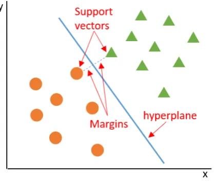
A support vector machine uses a hyperplane to separate two classes of data. It has been proven that the up-per bound of the generalization error of an SVM is low-ered if the margin is maximized [12]. The margin is the largest possible distance between the hyperplane and the instances on either side of this plane. A simplified example of an SVM can be found in Figure 1.

If the data would not be as perfectly spread as in Fig-ure 1, extra dimensions are added to be able to draw a hyperplane between the two possible classes. SVMs are binary and can only distinguish between two classes, how-ever, they can be used for multi-class problems. When an SVM is used for multi-class problems, the problem has to be reduced to a set of multiple binary classification prob-lems.

An advantage of SVMs is that they can handle a large number of features [12]. A few things to take into account with this classifier is that if there is data that was clas-sified wrongly or more noisy it could affect the accuracy negatively, as the drawing of a correct hyperplane will be-come more difficult, furthermore, the calculation/training time of a SVM can be very high.

3.2.2 Decision Tree

[image:3.595.324.533.59.236.2]

The decision tree algorithm generates a decision tree that classifies examples by sorting them based on their feature values [12]. Every node of a decision tree represents one of these features and every branch that comes from such

Figure 1. Simplified example of a support vector machine.

[image:3.595.312.543.409.520.2]

a node represents a possible value for that feature. Clas-sification of the examples starts at the top node of the tree, the root. Based on its feature values the example is then sorted to the leaves of the tree where it will be given a label. The features that contain the most information are placed near the root node. The efficiency of a decision tree is usually near-optimal and never completely optimal, because the production of the optimal decision tree is an NP-complete problem. An example of a decision tree can be seen in Figure 2.

Figure 2. Example of a decision tree

The advantages of the decision tree algorithm are that it is easy to comprehend and therefore quite fast, furthermore, decision trees work very well with discrete and categorical features. Something to take into account with this classi-fier is that if the features of the examples are numerical it can take a while for it to find the right threshold that decides when which branch of the tree is picked [12]. Fur-thermore, the decision tree is not very efficient when the number of examples is in the range of hundreds of thou-sands.

4. DATA COLLECTION

This section describes the collection of the data for this research.

4.1 Setup

(4)

all receiver and transmitter antenna pairs. The CSI tool worked with the 801.11n WiFi standard. A TP-LINK AC1750 Router was used, which worked with this WiFi standard. The receiver nodes that were used were created by Klein Brinke in his research [11]. The nodes were Giga-byte Brix IoTs, a type of mini PCs, of which the wireless cards of were replaced with the Intel Ultimate N Wi-Fi Link 5300, in order to make them work with the CSI tool. Both the router and the nodes had three antennas that could be used to transfer the CSI.

[image:4.595.326.522.49.491.2]

The layout of the setup of the experiment can be seen in Figure 6. The pictures in Figures 3, 4 and 5 show the position of the receiver nodes and the router in the room by means of pictures.

Figure 3. Setup experiment of day one.

4.2 Experiments

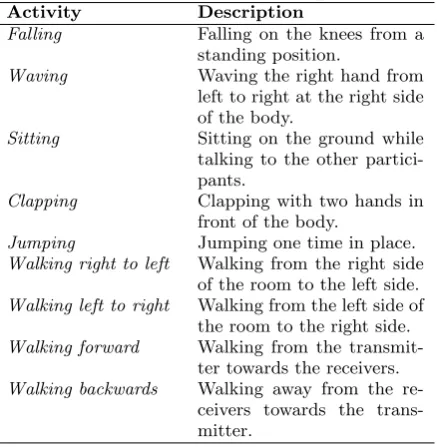
The experiments were divided over nine sessions which were divided over three days with three sessions each. For each session the general idea of the experiment consisted of a group of people performing the same activities at the same time in one room. The group would stand between a WiFi transmitter and one or more WiFi receivers. While the participants were performing the activities a stable WiFi signal between the router and the receivers would make sure that the CSI was collected and stored for later reference. For each session, there was a varying total group size of between four and seven participants, of which a per-centage of 50%, 75% or 100% of the group performed the same activity at the same time. All the participant groups consisted of different people, with some overlap between the groups. The groups performed the following activi-ties: falling, waving, sitting, clapping, jumping, walking from left to right, walking from right to left, walking for-ward and walking backfor-wards. A more detailed description of the activities can be found in Table 1. During each session every activity was repeated fifty times, to gather enough trials for the training of the classifiers in the data analysis process.

The stable WiFi signal mentioned, was needed to be able to see the change of the CSI over time. This stable signal was obtained by letting all the receiving nodes ping the router with an interval of 0.1 seconds during each trial. The CSI data was collected based on the packets that were sent back by the router to the receiver. For each trial of an activity, fifty of these ping messages were sent after each other by the receiver, making each trial last five seconds. The interval of 0.1 seconds was based on the re-search performed by Klein Brinke [11]. In his rere-search he used a ping interval of 0.05 seconds and every 100 packets would equal one trial. Because the research described in

Figure 4. Setup experiment of day two.

this paper worked with multiple nodes, the interval had to be increased. When running test experiments with two nodes, one of the nodes was removed from the network when both were sending ping messages at an interval of 0.05 seconds. When this interval was increased to 0.1 sec-onds, this did not happen anymore.

[image:4.595.72.267.216.364.2]

(5)

[image:5.595.71.267.51.200.2] [image:5.595.56.275.250.474.2]

Figure 5. Setup experiment of day three.

Table 1. Activities used in experiments

Activity Description

Falling Falling on the knees from a

standing position.

Waving Waving the right hand from

left to right at the right side of the body.

Sitting Sitting on the ground while

talking to the other partici-pants.

Clapping Clapping with two hands in

front of the body.

Jumping Jumping one time in place.

Walking right to left Walking from the right side of the room to the left side.

Walking left to right Walking from the left side of the room to the right side.

Walking forward Walking from the transmit-ter towards the receivers.

Walking backwards Walking away from the re-ceivers towards the trans-mitter.

positioned in the middle, stopped working.

Figure 6. Layouts of experiment setup.

The second aspect that was varied over the sessions was the percentage of the group that was actually performing the activity. This was done to find the effect of different percentages of the group performing the same activity on the performance of the classifiers (subquestion 2). The percentage of the group of participants performing the ac-tivities varied between 50%, 75% and 100%. In the case that not 100% of the group was performing the same activ-ity, the percentage of the group that was not performing the activity was walking in circles around the group per-forming the activities, to simulate disturbance of the WiFi signal by people performing different activities in real life. To illustrate, if the size of a participant group would be six and the percentage of the group performing the activ-ity would be fifty percent, then three participants would

perform the nine activities described above and the three other participants would walk around these participants. To answer the subquestion, the relation between the per-formance of the classifiers and the percentage of the group performing the same activity was analyzed in the classifi-cation process.

To find out to what extend one could measure the direction in which a group of people was moving (subquestion 3), the activities walking left to right, walking right to left,

walking forward and walking backwards were included in the research. By looking at the confusion matrices created in the classification process, it was possible to answer the question.

5. METHODOLOGY

For the analysis of the data the channel state matrices needed to be extracted from the packets that arrived at the receivers. This was done using the CSI tool released by Halperin et al. in 2011 [8]. This tool has been used in numerous research regarding activity classification using CSI [1, 4, 6, 20] and turned out to be a working software with extensive documentation.

The CSI was processed an classified using MATLAB [17]. MATLAB was used to train and test two classifiers: de-cision tree and support vector machine. These classifiers showed good results in previous research by Bagave [1] and Wang et al. [19] where they were used for single person ac-tivity recognition.

To find out what classifier had the highest performance when identifying the activity of a group of people (sub-question 4), the performances of the classifiers were com-pared in MATLAB. The performances were calculated us-ing the confusion matrices that resulted from the classifi-cation process. In MATLAB theF1score and accuracy of each classifier were calculated for every experiment session. By comparing the calculated performances the four sub-questions and the main research sub-questions were answered.

5.1 CSI extraction

It was not possible to immediately use the CSI values stored in the .dat files that were created by the third party CSI tool. The files first needed to be processed using meth-ods described on the website of the CSI tool [7]. To be able to get all the channel state matrices stored in a .dat file, the following method was called in MATLAB [17]:

read_bf_file(’name_of_csi_trace_file.dat’).

The variable created using this method,csi_trace, equalled a 1x302 cell array of which the first fifty entries were struc-tured arrays. Thesestructscontained the CSI data on the received packages for all the fifty frames used per trial of an activity. The remaining 252 cells that were created by the CSI tool contained no useful information and were therefore removed. One of the entries in thecsi_trace

file was inspected using the following code:

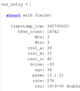
csi_entry = csi_trace{1}.

The value stored incsi_entryequalled a structured array with entries as can be seen in Figure 7.

[image:5.595.60.278.508.581.2]

(6)

[image:6.595.97.231.55.206.2]

Figure 7. The data stored on a package received by the receiver.

csi = abs(get_scaled_csi(csi_entry))

Thecsivariable obtained with this method was a 3x3x30 matrix that represented the MIMO channel state for this frame with positive values. The values of these CSI ma-trices were used to calculate the features.

5.2 Data preprocessing and cross validation

In the data preprocessing phase of the research, the chan-nel state matrices were used to calculate the features and compile tables that could serve as data sets for the classi-fiers. The following time domain features were selected for this research: the mean, the kurtosis, the standard devi-ation, the maximum, the minimum, the variance and the median. These features were calculated for every receiver antenna, transmitter antenna and subcarrier combination over the fifty frames that were collected for every trial. So, for every trial there were 3 * 3 * 30 =270 entries of which the features were calculated. To be able to reference each of these 270 instances back to one trial, every trial obtained a unique ID.

During the creation of these tables five-folds cross valida-tion was applied by creating five separate tables with equal amounts of data. For every activity, the trials were ran-domly divided over the five tables. For every experiment session, a separate set of tables was created containing the data with the features that were used to train the classi-fiers.

The result of the preprocessing were five tables per exper-iment session, with variables as represented in Table 2. In these tables all the unique combinations of Rx, Tx, Sub-carriers and Nodes had their own row.

5.3 Data classification

For the classification of the data the MATLAB templates were used for the support vector machine and the deci-sion tree classifiers. The parameters were kept at default values. The classification process was ran on a Lenovo Thinkpad T460s with an Intel Core i5 - 6200U proces-sor [18]. Because the high complexity of SVM and a large data set, it took very long for the laptop to train the SVM in a short time. Therefore, it was decided to train the clas-sifiers with one of training and testing set combinations for each experiment session. Furthermore, the classifiers were trained with 10 trials of the total number of 50 tri-als collected in the data collection process. When these trials were divided over the five tables, two trials per ac-tivity per table remained. After the training and testing

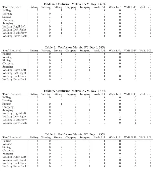
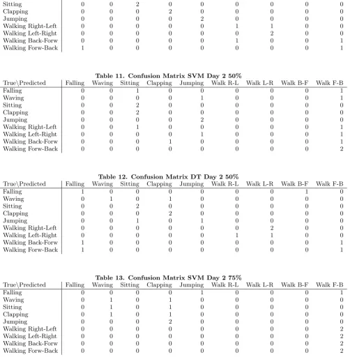
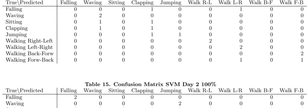
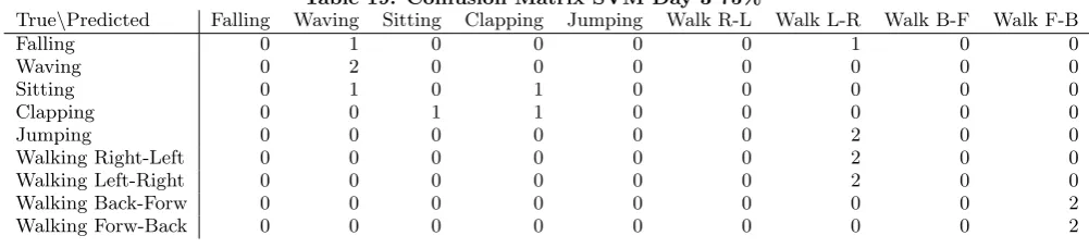
of the classifiers, confusion matrices were produced by the MATLAB script. These confusion matrices can be found in Section B.

5.4 Performance calculation

The performances of the classifiers was represented by the

F1 score and the accuracy of the confusion matrices that resulted from the testing phase of the classifiers. TheF1 score used the precision and recall of a confusion matrix and provided a balanced average of the two with a value between 0 and 1. To optimize the performance, the highest possible F1 score should be achieved. The F1 score was calculated using the following formula [15]:

F1= 2×

precision×recall precision+recall

The accuracy of the classifiers considers the true positives and negatives and the false positives and negatives to ob-tain a score between 0 and 1. The accuracy was repre-sented by the following formula:

Accuracy= tp+tn

tp+tn+f p+f n

To calculate theF1 scores and accuracies for the differ-ent classifiers for each experimdiffer-ent session, firstly the true positives, true negatives, false positives, false negatives, accuracy, precision, recall and F1 score were calculated for each of the individual activity classes. For the overall

F1 score and accuracy of an experiment session, the mean of the F1 scores and accuracies of the individual classes were calculated.

6. RESULTS AND DISCUSSION

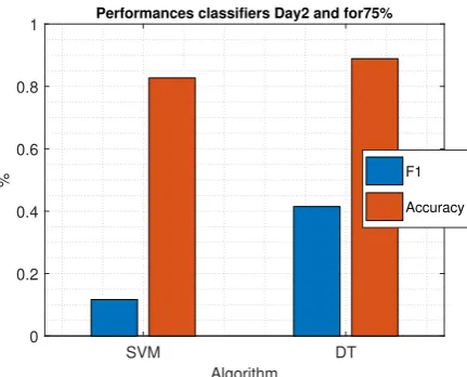
The training and testing of both the SVM and DT clas-sifiers with a data set consisting of 10 trials per activity class resulted in the accuracies displayed in Table 3 and the F1 scores displayed Table 4. The graphs displaying theF1 score and accuracy per classifier, per day and per percentage and the confusion matrices on which these per-formances are based can be found in appendix A and B, respectively. In the confusion matrices one could see that the different directions of walking could be distinguished from each other.

Overall the accuracy of an experiment session was above 80%, but almost all theF1scores were below 0.70. Which meant that the balance between the precision and recall of the classifiers was not optimal. The lowF1scores could be explained by extreme values in the precision and re-call. These extreme values in precision and recall could occur because there were 2 trials per activity in the testing dataset. This made the impact of one wrongly classified trial very big on the precision or recall.

(7)

Table 2. Table structure of the tables containing the training features

Label Trial Node Rx Tx Sub carrier Features...

Activity Label

The trial ID Receiving node

Receiver antenna

Transmitter antenna

Subcarrier used

One column for each of the features

Table 3. Accuracies of the classifiers for every combination of number of nodes and percentages

Percentage\Nodes 1 2 3

SVM DT SVM DT SVM DT

50 0.8272 0.9012 0.8519 0.8889 0.8519 0.9136 75 0.8889 0.9383 0.8272 0.8889 0.8642 0.9877 100 0.9383 0.9506 0.8889 0.9383 0.8765 0.9259

Table 4. F1 scores of the classifiers for every combination of number of nodes and percentages

Percentage\Nodes 1 2 3

SVM DT SVM DT SVM DT

50 0.1429 0.4778 0.179 0.4704 0.1983 0.6074 75 0.4196 0.6889 0.1166 0.4148 0.2531 0.9407 100 0.637 0.7333 0.4198 0.7 0.3333 0.6185

not run a test experiment to check whether the accuracy achieved by one participant group could be compared to another participant group. Another cause could be that the number of trials that were useds for the training of the classifiers was too little to see a clear influence in the performances for the classifiers.

The influence of the number of nodes on the performance of the classifiers was also expected to be higher, because data from more different angles would give the classifiers more information to work with and, thus, the possibility for higher performances. This influence being very minor, could have been caused by the amount of trials per class, as more data could potentially get better results. Fur-thermore, the different composition of all the participant groups could also be a cause of this, like for the influence of the percentage.

In general the decision tree had a higher accuracy andF1 score than the support vector machine and thus better results. Furthermore, the support vector machine algo-rithm had a very high complexity, which made it take hours to train the classification model, where the decision tree would take less than a minute. The support vec-tor machine might have been outperformed by decision tree, because SVMs require careful parameter selection as stated by Caruana et al. [3], and in this research these parameters were kept at their default values.

7. CONCLUSION AND FUTURE WORK

The main research question addressed in this research was: To what extend can one recognize what activity the biggest part of a group of people is performing using channel state information? To answer the main question of this paper, firstly the subquestions are answered.

The first subquestion was: What is the correlation be-tween the amount of receivers and the performance of the classifiers? By looking at Tables 3 and 4, one can deduce that the amount of nodes used for the experiments, does not explicitly influence the accuracy or theF1score of the classifiers. There appears to be no clear relation between the amount of nodes and the performance of the classifiers, however, no conclusions can be drawn for this subquestion from the results of this research, as the amount of data used in this research was not enough. More research is necessary in order to get more evident results.

The second subquestion was: What is the effect of different percentages of the group performing the same activity on the performance of the classifiers? By analyzing Tables 3 and 4 it becomes clear that the F1 score and the accu-racy of a session increases with the percentage of a group performing the same activity. However, there are some exceptions, for example, On day 3, the session where 75% of the people performed the main activity, the accuracy andF1 score were higher than the sessions where 50% and 100% of the people were performing the main activity.

The third subquestion was: To what extend can we mea-sure the direction in which a group of people is moving? This question can be answered by looking at the confu-sion matrices in Section B. From these confuconfu-sion matrices one can deduce that it is indeed possible for the classifier to identify in which direction the group of participants is moving. However, the amount of data that was collected in this research was not enough to get a very clear distinc-tion, but it appears to be possible.

The fourth subquestion was: What classifier has the high-est performance when identifying the activity of the group? The classifier with the highest performance is clearly the decision tree algorithm. It has a higherF1score and accu-racy than SVM in all of the test scenarios. Furthermore, the calculation time of the decision tree classifier was small in comparison to the one of support vector machine, which makes it even more preferred.

To conclude, it is possible to recognize activities performed by the biggest part of a group of people. The decision tree classifier gives good results and short computation time and can therefore be used for group activity recognition. It is possible to recognize the activity performed by only 50% of a group of people and it is possible to recognize the direction in which a group of people is moving. Regarding the number of nodes, no clear conclusion can be drawn, however, based on the current results there appears to be no clear relation between the number of nodes and the performance of the classifier.

(8)

the best for group activity recognition. Additionally, re-searchers could look deeper into the identification of the direction of a group of people with more data and even smaller percentages could be investigated regarding activ-ity recognition to see the effects on the performance of the classifiers.

8. REFERENCES

[1] P. Bagave. Unobtrusive sensing using wifi signals. August 2018.

[2] J. Beckett. Can a computer write a hit musical? thanks to machine learning, we’re about to find out.

https://blogs.nvidia.com/blog/2016/01/14/ musical-machine-learning-gpus/. Accessed: 2018-11-13.

[3] R. Caruana and A. Niculescu-Mizil. An empirical comparison of supervised learning algorithms. In

Proceedings of the 23rd international conference on Machine learning, pages 161–168, 2006.

[4] C. Du, X. Yuan, W. Lou, and Y. Thomas Hou. Context-free fine-grained motion sensing using wifi.

2018 15th Annual IEEE International Conference on Sensing, Communication, and Networking, SECON 2018, pages 1–9, 2018.

[5] I. Fadelli. Improbotics: Bringing machine intelligence into improvised theatre.

https://techxplore.com/news/

2018-09-improbotics-machine-intelligence-theatre. html. Accessed: 2018-11-13.

[6] C. Feng, S. Arshad, and Y. Liu. Mais: Multiple activity identification system using channel state information of wifi signals.Lecture Notes in

Computer Science (including subseries Lecture Notes in Artificial Intelligence and Lecture Notes in Bioinformatics), 10251 LNCS:419–432, 2017. [7] D. Halperin. FAQ, things to know, and

troubleshooting.https://dhalperi.github.io/ linux-80211n-csitool/installation.html. Accessed: 2019-01-19.

[8] D. Halperin, W. Hu, A. Sheth, and D. Wetherall. Tool release: Gathering 802.11n traces with channel state information.Computer Communication Review, 41(1):53, 2011.

[9] K. K. Htike, O. O. Khalifa, H. A. M. Ramli, and M. A. Abushariah. Human activity recognition for video surveillance using sequences of postures. In

3rd International Conference on e-Technologies and

Networks for Development, ICeND 2014, pages 79–82, 2014.

[10] B. Jia, J. Li, and H. Xu. Pshcar: A

position-irrelevant scene-aware human complex activities recognizing algorithm on mobile phones.

Communications in Computer and Information Science, 901:192–211, 2018.

[11] J. Klein Brinke. Device-free sensing and deep learning: Analysing human behaviour through csi using convolutional networks. 2018.

[12] S. B. Kotsiantis, I. Zaharakis, and P. Pintelas. Supervised machine learning: A review of classification techniques.Emerging artificial intelligence applications in computer engineering, 160:3–24, 2007.

[13] M. Kwon and S. Choi. Recognition of daily human activity using an artificial neural network and smartwatch.Wireless Communications and Mobile Computing, 2018.

[14] M. Mobark, S. Chuprat, T. Mantoro, and A. Azizan. Utilization of mobile phone sensors for complex human activity recognition.Advanced Science Letters, 23(6):5466–5471, 2017.

[15] Y. Sasaki. The truth of the f-measure. 2007. [16] Unknown. Fitbit.

https://www.fitbit.com/nl/home. Accessed: 2019-01-25.

[17] Unknown. Matlab.https:

//www.mathworks.com/products/matlab.html. Accessed: 2018-12-02.

[18] Unknown. Thinkpad t460s.https:

//www.lenovo.com/nl/nl/laptops/thinkpad/ t-series/ThinkPad-T460s/p/22TP2TT460S. Accessed: 2019-01-30.

[19] C. Wang, S. Chen, Y. Yang, F. Hu, F. Liu, and J. Wu. Literature review on wireless sensing-wi-fi signal-based recognition of human activities.

Tsinghua Science and Technology, 23(2):203–222, 2018.

[20] J. Wang, H. Jiang, J. Xiong, K. Jamieson, X. Chen, D. Fang, and B. Xie. Lifs: low human-effort, device-free localization with fine-grained subcarrier information. 0(1):243–256, 2016.

(9)

APPENDIX

A. PERFORMANCES

SVM DT

Algorithm 0

0.2 0.4 0.6 0.8 1

%

Performances classifiers Day1 and for50%

F1

[image:9.595.317.534.51.225.2]

Accuracy

Figure 8. Graph showing performance of the clas-sifiers on Day 1 with 50% of the participants

SVM DT

Algorithm 0

0.2 0.4 0.6 0.8 1

%

F1

[image:9.595.58.281.57.262.2]

Accuracy

SVM DT

Algorithm 0

0.2 0.4 0.6 0.8 1

%

F1

Accuracy

SVM DT

Algorithm 0

0.2 0.4 0.6 0.8 1

%

F1

[image:9.595.317.533.280.454.2]

Accuracy

SVM DT

Algorithm 0

0.2 0.4 0.6 0.8 1

%

F1

[image:9.595.62.281.313.488.2]

Accuracy

SVM DT

Algorithm 0

0.2 0.4 0.6 0.8 1

%

F1

Accuracy

[image:9.595.317.534.509.684.2] [image:9.595.62.281.541.713.2]

(10)

SVM DT Algorithm

0 0.2 0.4 0.6 0.8 1

%

F1

[image:10.595.318.533.51.225.2]

Accuracy

SVM DT

Algorithm 0

0.2 0.4 0.6 0.8 1

%

F1

[image:10.595.62.280.51.225.2]

Accuracy

SVM DT

Algorithm 0

0.2 0.4 0.6 0.8 1

%

F1

[image:10.595.62.280.278.452.2]

Accuracy

(11)

[image:11.595.51.554.73.640.2]

B. CONFUSION MATRICES

Table 5. Confusion Matrix SVM Day 1 50%

True\Predicted Falling Waving Sitting Clapping Jumping Walk R-L Walk L-R Walk B-F Walk F-B

Falling 0 1 1 0 0 0 0 0 0

Waving 0 0 0 1 0 1 0 0 0

Sitting 0 1 1 0 0 0 0 0 0

Clapping 0 1 0 1 0 0 0 0 0

Jumping 0 1 1 0 0 0 0 0 0

Walking RigH-Left 0 0 0 0 0 0 0 0 2

Walking Left-Right 0 0 1 0 0 0 0 0 1

Walking Back-Forw 0 0 1 0 0 0 0 0 1

Walking Forw-Back 0 0 0 0 0 0 0 0 2

Table 6. Confusion Matrix DT Day 1 50%

Falling 1 0 1 0 0 0 0 0 0

Waving 1 0 0 1 0 0 0 0 0

Sitting 0 0 1 0 1 0 0 0 0

Clapping 0 0 0 2 0 0 0 0 0

Jumping 0 0 0 0 2 0 0 0 0

Walking Right-Left 0 0 0 0 1 0 1 0 0

Falling 0 0 0 1 1 0 0 0 0

Waving 0 1 0 1 0 0 0 0 0

Sitting 0 0 1 1 0 0 0 0 0

Clapping 0 0 0 2 0 0 0 0 0

Jumping 0 0 0 0 1 0 0 1 0

Falling 2 0 0 0 0 0 0 0 0

Waving 0 2 0 0 0 0 0 0 0

Sitting 0 0 2 0 0 0 0 0 0

Clapping 0 0 0 2 0 0 0 0 0

Jumping 0 0 0 0 1 0 0 1 0

(12)

Falling 0 0 0 0 2 0 0 0 0

Waving 0 2 0 0 0 0 0 0 0

Sitting 0 1 1 0 0 0 0 0 0

Clapping 0 0 0 2 0 0 0 0 0

Jumping 0 0 0 0 2 0 0 0 0

Falling 2 0 0 0 0 0 0 0 0

Waving 0 2 0 0 0 0 0 0 0

Sitting 0 0 2 0 0 0 0 0 0

Clapping 0 0 0 2 0 0 0 0 0

Jumping 0 0 0 0 2 0 0 0 0

[image:12.595.55.555.255.778.2]

Falling 0 0 1 0 0 0 0 0 1

Waving 0 0 0 0 1 0 0 0 1

Sitting 0 0 2 0 0 0 0 0 0

Clapping 0 0 2 0 0 0 0 0 0

Jumping 0 0 0 0 2 0 0 0 0

Falling 1 0 0 0 0 0 0 1 0

Waving 0 1 0 1 0 0 0 0 0

Sitting 0 0 2 0 0 0 0 0 0

Clapping 0 0 0 2 0 0 0 0 0

Jumping 0 0 1 0 1 0 0 0 0

Falling 0 0 0 0 1 0 0 0 1

Waving 0 1 0 1 0 0 0 0 0

Sitting 0 1 0 1 0 0 0 0 0

Clapping 0 1 0 1 0 0 0 0 0

Jumping 0 0 0 2 0 0 0 0 0

(13)

[image:13.595.50.554.80.258.2]

Table 14. Confusin Matrix DT Day 2 75%

Falling 0 0 0 1 0 0 1 0 0

Waving 0 2 0 0 0 0 0 0 0

Sitting 0 1 0 1 0 0 0 0 0

Clapping 0 1 0 1 0 0 0 0 0

Jumping 0 0 0 1 1 0 0 0 0

[image:13.595.49.551.208.781.2]

Falling 2 0 0 0 0 0 0 0 0

Waving 0 0 0 0 2 0 0 0 0

Sitting 0 0 2 0 0 0 0 0 0

Clapping 0 0 1 1 0 0 0 0 0

Jumping 1 0 0 0 1 0 0 0 0

Falling 2 0 0 0 0 0 0 0 0

Waving 0 2 0 0 0 0 0 0 0

Sitting 0 0 2 0 0 0 0 0 0

Clapping 0 0 0 2 0 0 0 0 0

Jumping 0 0 0 0 2 0 0 0 0

Falling 0 0 0 0 0 0 0 0 2

Waving 0 2 0 0 0 0 0 0 0

Sitting 0 1 0 0 0 0 0 0 1

Clapping 0 0 1 0 1 0 0 0 0

Jumping 0 0 0 0 2 0 0 0 0

Falling 0 0 0 0 0 0 0 0 2

Waving 0 2 0 0 0 0 0 0 0

Sitting 0 1 1 0 0 0 0 0 0

Clapping 0 0 0 2 0 0 0 0 0

Jumping 0 0 0 0 2 0 0 0 0

(14)

[image:14.595.52.553.93.207.2]

Falling 0 1 0 0 0 0 1 0 0

Waving 0 2 0 0 0 0 0 0 0

Sitting 0 1 0 1 0 0 0 0 0

Clapping 0 0 1 1 0 0 0 0 0

Jumping 0 0 0 0 0 0 2 0 0

Falling 2 0 0 0 0 0 0 0 0

Waving 0 2 0 0 0 0 0 0 0

Sitting 0 0 2 0 0 0 0 0 0

Clapping 0 0 0 2 0 0 0 0 0

Jumping 0 0 0 0 2 0 0 0 0

Falling 0 0 0 0 0 0 2 0 0

Waving 0 0 2 0 0 0 0 0 0

Sitting 0 0 1 1 0 0 0 0 0

Clapping 0 0 1 1 0 0 0 0 0

Jumping 0 0 0 0 2 0 0 0 0

Falling 0 0 0 0 0 1 1 0 0

Waving 0 2 0 0 0 0 0 0 0

Sitting 0 0 2 0 0 0 0 0 0

Clapping 0 0 0 2 0 0 0 0 0

Jumping 0 0 0 0 2 0 0 0 0