University of Warwick institutional repository: http://go.warwick.ac.uk/wrap
This paper is made available online in accordance with publisher policies. Please scroll down to view the document itself. Please refer to the repository record for this item and our policy information available from the repository home page for further information.
To see the final version of this paper please visit the publisher’s website. Access to the published version may require a subscription.
Author(s): Mark Britten-Jones, Anthony Neuberger and Ingmar Nolte Article Title: Improved Inference and Estimation in Regression With Overlapping Observations
Year of publication: Forthcoming
Link to published version: Not yet published
Publisher statement: This article has been accepted for publication in
Improved Inference and Estimation in Regression With
Overlapping Observations
Mark Britten-Jones
∗BlackRock Global Investors
Anthony Neuberger
†Warwick Business School,
FERC, FORC
Ingmar Nolte
‡Warwick Business School,
FERC, CoFE
This version: March 3, 2010
∗Managing Director, BlackRock Global Investors, Murray House, 1 Royal Mint Court, London EC3N 4HH, United Kingdom. Phone +44-20-7668-8965, email: [email protected].
†Corresponding author: Warwick Business School, Finance Group, University of Warwick, CV4 7AL, Coventry, United Kingdom. Phone +44-24-765-22955, Fax -23779, email: [email protected].
Improved Inference and Estimation in Regression With
Overlapping Observations
Abstract
We present an improved method for inference in linear regressions with overlapping
observations. By aggregating the matrix of explanatory variables in a simple way, our
method transforms the original regression into an equivalent representation in which
the dependent variables are non-overlapping. This transformation removes that part
of the autocorrelation in the error terms which is induced by the overlapping scheme.
Our method can easily be applied within standard software packages since conventional
inference procedures (OLS-, White-, Newey-West- standard errors) are asymptotically
valid when applied to the transformed regression. Through Monte Carlo analysis we
show that they perform better in finite samples than the methods applied to the original
regression that are in common usage. We illustrate the significance of our method with
two empirical applications.
JEL classification: C20, G12
1
Introduction
Researchers in empirical finance often regress long-horizon returns onto explanatory variables.
Such regressions have been used to assess stock return predictability, to test the expectations
theory of the term structure of interest rates, to test the cross-sectional pricing implications of
the CAPM and consumption-CAPM, to investigate the forward premium puzzle, and to test
the efficiency of foreign exchange markets. These regressions involve overlapping observations
which raise econometric issues that are addressed in this paper.
Regressions with long horizon returns often show much higher R2’s than regressions with
one-period returns. But work by Valkanov (2003), Hjalmarsson (2006), and Boudoukh,
Richardson & Whitelaw (2008) suggests that long-horizon return regressions have no greater
statistical power to reject the null of no predictability than their short-horizon counterparts.
For testing predictability the use of long-horizon returns (as opposed to one-period returns)
would appear to be of little value.
Nonetheless, the analysis of long-horizon returns can contribute significantly to understanding
predictability (or dependence) and its economic significance. For example, one concern with
the interpretation of short-horizon regressions is measurement error. Cochrane & Piazzesi
(2005, p. 139) forecast annual bond returns using monthly data and claim that “to see the
core results you must look directly at the one-year horizon” and further find that estimating
a typical one-month return model “completely misses the single factor representation” due to
measurement error. Another reason for analyzing longer horizons is lengthy and uncertain
response times. A number of recent studies of the consumption-CAPM, including Daniel
& Marshall (1997), Parker (2001), Parker & Julliard (2005), Jagannathan & Wang (2005,
2007), and Malloy, Moskowitz & Vissing-Jorgensen (2005) measure consumption risk using
works better than the standard consumption-CAPM. If consumers face costs associated with
changing consumption, or if information acquisition is constrained, then consumption may
change more slowly than implied by the standard consumption-CAPM, and this justifies a
focus on returns and consumption growth measured over longer horizons.
Long-horizon return regressions potentially suffer from two econometric problems. The first
is bias in the usual OLS coefficient estimates. The bias is not caused by the presence of
over-lapping observations but arises when the predictor variable is persistent and its innovations
are strongly correlated with returns (see Gregory Mankiw & Shapiro (1986) and Stambaugh
(1999)). These conditions may also arise in short-horizon regressions.
Our paper does not address this problem of bias but focuses instead on the second problem,
one which is specific to overlapping observations: the strong autocorrelation pattern induced
by the overlapping scheme. It is now well known that commonly used methods to deal with
the autocorrelation are inadequate and can lead to misleading estimates of the confidence
intervals associated with coefficient estimates obtained from finite samples. Despite this,
many studies still resort to standard inference techniques such as applying White or common
Newey-West standard errors within an overlapping regression framework.1
This paper presents a simple procedure that can markedly improve inference in regressions
with overlapping observations. The beauty of our approach, for practical purposes, is that it
can be readily implemented in standard econometric software packages and no serious
pro-gramming is needed to obtain our inference statistics.
We consider an overlapping regression in which a multi-period return is regressed onto a set
1
of regressors, and for which observations are available each period. This regression is
trans-formed into a non-overlapping regression in which one-period returns are regressed onto a set
of transformed regressors. The OLS coefficient estimates from the original and transformed
regressions are numerically identical, but inference based on the transformed regression is
sim-plified because the autocorrelation induced by overlapping observations is no longer present.
The procedure is equally applicable to time-series regressions and to panel regressions. It can
be applied to both predictive (forecasting) and contemporaneous (explanatory) regressions.
We show that standard inference procedures, such as OLS, White (1980) and Newey &
West (1987), are asymptotically valid when applied to the transformed regression. To
as-sess the finite-sample performance of our procedure we run Monte Carlo simulations. These
show that the standard inference procedures perform substantially better when based on the
transformed regression rather than on the original specification. Indeed, simpler procedures,
such as OLS and White, when applied to the transformed regression, perform better than
more sophisticated techniques such as Hansen & Hodrick (1980) and Newey-West applied to
the original regression. The superior performance of our procedure is most marked when the
return horizon in the original specification is long in comparison to the sample length, and
Hansen-Hodrick and Newey-West standard errors tend to be severely biased down. The
stan-dard errors obtained from our transformed regression have much less bias and lower stanstan-dard
deviation. The result is that confidence intervals using our method have coverage
probabili-ties much closer to their nominal levels than confidence intervals constructed using standard
techniques.
Other papers have documented problems with conventional inference applied to long-horizon
regressions (for example Ang & Bekaert (2007), Nelson & Kim (1993), and Hodrick (1992))
litera-ture develops covariance estimators for specific cases, imposing additional struclitera-ture on the
serial correlation of moment conditions. These structured estimators generally have
excel-lent small-sample properties, but their applicability is limited. For example, the estimator
of Richardson and Smith (1991) provides valid inference only under the null hypothesis that
returns are serially uncorrelated, and only when the explanatory variables are past returns.
Even then, valid inference requires the unpalatable assumption (for asset returns) of
condi-tional homoscedasticity.
The methodology that is most similar to ours is Hodrick (1992). He presents a structured
co-variance estimator that generalizes Richardson & Smith (1991) in that regressors need not be
past returns and returns need not be conditionally homoscedastic. A drawback of Hodrick’s
derivation is that it is complex, and as a result his estimator has not gained widespread
acceptance. For example Campbell, Lo & MacKinlay (1997) do not mention it in their
well-known textbook, despite having a detailed discussion on statistical inference in long-horizon
regressions. It has also not been widely used in the empirical literature, with the exception of
Ang & Bekaert (2007). They use Hodrick (1992) standard errors and argue that much of the
empirical evidence for the time-series predictability of stock returns has been overstated in the
literature due, in part, to the use of OLS or Hansen & Hodrick (1980) standard errors which
they find ’lead to severe over-rejections of the null hypothesis’. Our method is not complex,
easy to implement and therefore is more likely to be adopted by empirical researchers.
Our method naturally extends to cases where the error term in short-horizon regressions is
autocorrelated. By transforming the regression equation, the autocorrelation in the error
term induced by the use of overlapping data is stripped out. The researcher can then focus
on addressing any remaining autocorrelation present in short-horizon returns by applying the
Jegadeesh (1991) and Cochrane (1991) advocate an approach which is similar in appearance
to ours. They bypass the problem of overlapping observations by regressing one-period
re-turns onto the sum of lags of the explanatory variable. However, this is strictly a procedure
for testing the null of no-predictability. It does not provide a coefficient estimate for a
long-horizon regression, and it is restricted to regressions with a single explanatory variable, so it
is of little use for understanding the sources of long-horizon predictability.
Our approach is particularly useful for panel data, where the complexity and size of the data
precludes some of the more sophisticated methods for dealing with overlapping observations
such as bootstrapping and the Hodrick (1992) procedure. The Fama-MacBeth methodology
is a simple approach that neatly accounts for cross-sectional correlation in errors. When
multi-period returns are involved, we can use our transformed regression approach in
com-bination with the Fama-MacBeth methodology to remove the serial correlation induced by
overlapping observations.
Section 2 develops the basic idea in the context of inference for a linear regression with
over-lapping observations. Section 3 presents results from Monte Carlo studies demonstrating the
advantages of our approach. Section 4 illustrates our approach with two empirical examples.
The first example analyses the predictability of long-horizon US stock market returns and the
second example analyses reversal in relative country stock index returns. Section 5 concludes.
2
Linear Regression with Overlapping Observations
Letrdenote theT×1 vector of one period log returns andAthe (T−k+ 1)×T matrix, that has entriesaij = 1 ifi≤j ≤i+k−1 and 0’s otherwise, withi= 1, . . . , T−k+ 1. Thus, A is
and 0’s otherwise. Hence,Ar is the (T−k+ 1)×1 vector ofkperiod log returns2. X denotes
the (T −k+ 1)×ℓ matrix of explanatory variables (with the first column of X consisting of 1’s). We consider the following (predictive) linear regression setup with overlapping returns
Ar=Xβ+u, (1)
in which u denotes the (T −k+ 1)×1 error term vector. The OLS parameter estimate ofβ
in equation (1) is given by
ˆ
β= (X′X)−1X′Ar. (2) It can be rewritten as
ˆ
β= (X′X)−1(A′X)′r, (3) which shows that the OLS estimate of β can be rewritten in terms of the original non-overlapping one period returns.
Moreover, ˆβ as given in equation (3) can be obtained from an associated transformed regres-sion
r = ˜Xβ+ ˜u, (4)
in which ˜X is the T ×ℓ matrix of transformed explanatory variables given by ˜
X ≡A′X(X′AA′X)−1X′X, (5) and ˜u is theT ×1 error term vector of this transformed regression.3 To see this, note that
2We assume that the single period returns as well as the overlapping long period returns are available to the
researcher. This is generally the case, though the Hansen & Hodrick (1980) study of the foreign exchange market is an exception since the returns in that case are on three month forward contracts, and the prices of one week forward contracts are not available.
3
the OLS estimate ofβ in equation (4) is given by ˆ
β = ( ˜X′X˜)−1X˜′r,
= (X′X(X′AA′X)−1X′AA′X(X′AA′X)−1X′X−1
X′X(X′AA′X)−1X′Ar,
= (X′X)−1X′Ar, (6)
which is indeed the same as the estimator in equation (2).
Substituting for Ar from (1) into (2), and for r from (4) into (6) gives the following pair of equations for the error in the estimate ofβ which conventional inference procedures are based on:
ˆ
β−β = (X′X)−1X′u, ˆ
β−β = (X′X)−1X′Au.˜ (7) The benefit of using the second formulation is that the error depends explicitly on the
autocor-relation structure of ˜u, the noise in the transformed, non-overlapping regression, rather than onu, the noise in the overlapping regression. The autocorrelation structure of ˜u is generally much simpler than the autocorrelation structure of u since that part of the autocorrelation in u induced by the deterministic aggregation scheme A is explicitly known and accounted for. The efficiency gain lies in accounting for a known dependence pattern explicitly, without
the need to estimate it in a noisy way.
We do not claim that either model (1) or model (4) is the true data generating process. If
model (1) is misspecified so will be model (4) and thus issues such as inconsistency, bias,
endogeneity and omitted variable problems, are not addressed and cannot be mitigated by
the use of our transformation. However, our transformation will be of particular help in
improving the accuracy of the standard errors when the model is misspecified, because the
deal with this autocorrelation by itself (as in the transformed regression) rather than to deal
with both it and the autocorrelation induced by the use of overlapping observations at the
same time.
2.1
Inference on
β
We now show how the asymptotic covariance matrix of ˆβderived from the overlapping regres-sion (1) is related to the asymptotic covariance matrix of ˆβ derived from the non-overlapping regression (4). Let ˆβ(T−k+1) denote the OLS estimate ofβfrom a data sample of size T−k+ 1
obtained from regression equation (1). Rearranging equation (1) yields
T −k+ 1
√
T −k+ 1
ˆ
β(T−k+1)−β
=
1
T −k+ 1X ′X
−1 1
√
T −k+ 1X ′u,
and under certain regularity conditions4 we obtain a central limit theorem of the following
form
D−(T1−/2k+1)βˆ(T−k+1)−β
asy
∼ N(0, Iℓ),
with
D(T−k+1) =
1
T −k+ 1Q −1
(T−k+1)S(T−k+1)Q−(T1−k+1),
whereQ(T−k+1) is given by
Q(T−k+1) ≡E
1
T −k+ 1X ′X
,
and S(T−k+1) is given by
S(T−k+1) ≡ V
1
√
T −k+ 1X ′u
= T
T −k+ 1V
1
√
T(A
′X)′u˜
= T
T −k+ 1S˜(T).
4
The second line follows by exploiting the relationship in (7), and it links the asymptotic
covariance matrix S(T−k+1) in the overlapping regression with its twin asymptotic
covari-ance matrix ˜S(T) in the non-overlapping regression in which the deterministic transformation
scheme A is explicitly visible. Under the assumption of consistent estimates ˆ˜S(T) for ˜S(T)
and ˆQ(T−k+1) estimated by ˆQ(T−k+1) = T−1k+1X′X, a consistent estimate for the asymptotic
covariance matrix of ˆβ can be obtained by ˆ˜
D(T−k+1) =
T
(T −k+ 1)2Qˆ
−1
(T−k+1)Sˆ˜(T)Qˆ −1
(T−k+1). (8) Alternatively it can be obtained under the assumption of consistent estimates ˆS(T−k+1) for
S(T−k+1) as
ˆ
D(T−k+1) =
1
T −k+ 1Qˆ −1
(T−k+1)Sˆ(T−k+1)Qˆ−(T1−k+1).
In this latter case, we do however lose the advantage of accounting for the deterministic
trans-formation scheme A a priori and the estimate ˆS(T−k+1) will not be as precise as the estimate ˆ˜
S(T).
The most common procedure to estimate the covariance matrix of ˆβ under the suspicion of an unknown autocorrelation pattern in the error terms of a linear regression is to resort to the
Newey-West HAC covariance matrix. The Newey-West covariance estimate of ˆ˜S(T) is given
by
ˆ˜
S(T)= ˆΓA′X(0) + J X
j=1
w(j, J)ΓˆA′X(j) + ˆΓA′X(j)′
, (9)
with
ˆ
ΓA′X(j)≡ T−j X
t=1
(A′X)′
tuˆ˜tuˆ˜t+j(A′X)t+j,
and
w(j, J)≡1− j
where J denotes the lag length and a subscript t denotes the tth row of a matrix. From the
definition of ˜X in equation (5) it can be seen that ˜
Xt(X′X)−1(X′AA′X) = (A′X)t,
so that
ˆ
ΓA′X(j) = (X′AA′X)(X′X)−1ΓˆX˜(j)(X′X)−1(X′AA′X).
Substituting this expression into equation (9) and afterwards into equation (8) yields
ˆ˜
D(T−k+1) =T( ˜X′X˜)−1 ΓˆX˜(0) +
J X
j=1
w(j, J)ΓˆX˜(j) + ˆΓX˜(j)′
!
( ˜X′X˜)−1, (10)
which is the standard Newey-West HAC covariance matrix for the transformed non-overlapping
regression. This estimator is simple, it is consistent and it is guaranteed to be positive
def-inite. Without further knowledge of the autocorrelation structure in the error terms that
remains after correcting for the autocorrelation induced by the transformation A, it is the most reliable estimator at hand.
The White heteroscedasticity consistent covariance matrix is obtained as a special case (J = 0) and can be used under the assumption of no further autocorrelation in the error terms ˜u. In this case equation (10) simplifies to
ˆ˜
D(T−k+1) =T( ˜X′X˜)−1ΓˆX˜(0)( ˜X′X˜)−1. (11)
Our result is of key interest for practical purposes, since it shows that reliable standard errors
in the case of regressions with overlapping observations can be obtained simply by i)
con-structing the transformed regressor matrix ˜X, ii) running regression (4) and iii) relying on conventional Newey-West HAC standard errors on the basis of this regression for parameter
inference. The beauty of this is that it can be achieved almost effortlessly in any standard
3
Monte Carlo Analysis
We have outlined the relationship between the asymptotic covariance ofβ in the transformed and the overlapping regression. We argued that accounting for a known transformation
scheme a priori as done by the transformed regression will yield more precise estimates of
the covariance ofβ than applying conventional methods such as Hansen-Hodrick or Newey-West directly to the overlapping regression. In this section we show that inference based
on the transformed regression has indeed better finite-sample properties than conventional
approaches based on the overlapping regression.
We run Monte Carlo simulations using a variety of values forkand for the length of the data
T. We compare the performance of procedures based on the transformed regression with the more conventional approaches based on Newey-West and Hansen-Hodrick estimators of the
covariance matrix ofβ applied to the overlapping data regression.5
An alternative approach to improving the inference in the presence of auto-correlated
er-rors is to use pre-whitening, as in Andrews & Monahan (1992) and Sul, Phillips & Choi
(2005). In our simulations, pre-whitening at best performs comparably with the
Newey-West and Hansen-Hodrick estimators applied also to the overlapping regressions. For the
shorter datasets we consider, the estimation of the pre-whitening VAR comes so close to
non-stationarity that the estimated standard error is unstable. In the interests of space,
the simulations with the four alternative HAC estimators and with pre-whitening are not
reported here but are available from the authors’ website.
5
Our main finding is that the transformation we propose does indeed lead to substantial
improvements in inference for small samples. Conventional OLS standard errors obtained
from the transformed regression provide the most accurate small-sample inference for
ho-moscedastic data generating processes. In the presence of heteroscedasticity, White (1980)
heteroscedasticity-consistent standard errors from the transformed regression provide the
most accurate inference in small samples. For the case of autocorrelated error terms in
the non-overlapping data Newey & West (1987) from the transformed regression performs
best. When the forecast return horizon is long in comparison to the sample period, and when
the regressors are strongly positively autocorrelated, the Newey-West and Hansen-Hodrick
procedures produce standard errors that are severely biased downwards.
The underlying data generating process for our simulations of the one period return process
takes the following form
rt+1 =α+γ1X1t+νt+1,
where X1t is a stationary AR(1) processes with unit variance and AR parameter 0.8. We
consider four particular cases:
1) In the base case (Table 1) there is no predictability at any horizon (γ1 = 0) and the error
termνt+1 ∼N(0,1).
2) In the second case (Table 2) there is no predictability as in 1), but the error termνt+1 is
heteroscedastic with νt+1 =X1tεt+1, where εt+1 ∼N(0,1).
3) In the third case (Table 3) returns are predictable (γ1 = 0.5) and the error term νt+1 ∼
4) The fourth case (Table 4) is included to show the implications of autocorrelation in the
non-overlapping observations. We induce the autocorrelation by using a misspecified model.
Returns are predictable as in 3), but instead ofX1t a false regressorX2t is used in the
regres-sions. X2t is mutually uncorrelated with X1t and also follows a stationary AR(1) processes
with unit variance and AR parameter 0.8.
We consider two scenarios for the choice of the sample length T and overlapping periods k. The first scenario isT = 250 and k= 3; and the second scenario isT = 100 and k= 12. The overlapping regression in equation (1) is estimated. The standard error on ˆβ1 is reported. For
each data generating process, and for each sample length and return horizon we present
re-sults for four conventional covariance estimators applied to the overlapping regression: ’OLS’
is the standard OLS covariance estimator, ’White’ is the White (1980)
heteroscedasticity-consistent covariance estimator, ’NW’ is the Newey & West (1987) heteroscedasticity and
autocorrelation consistent (HAC) estimator, and ’HH’ is the heteroscedasticity-consistent
version of Hansen & Hodrick (1980). The choice of bandwidth for HAC estimators depends
on the assumed correlation structure. With an overlapping regression it is conventional to
use a bandwidth equal to the overlap or twice the overlap (see for example Cochrane &
Pi-azzesi (2005)). Since there is no qualitative difference between the results for a lag length
equal to J =k or J = 2k we only report the first case ’NW(k)’. In addition, we also report Newey-West standard errors ’NW’ with the common lag length as suggested by Newey &
West (1987), which is J =j4 T
100
2/9k
.
We then present results for covariance estimators based on the transformed regression. We
consider the three estimators presented in the previous section: OLS, White, and Newey-West.
For each covariance estimator and each scenario we report the bias, standard deviation, and
95%, and 90% regression coefficient confidence intervals. 50000 simulations are used for each
scenario.
Table 1 shows that the OLS and White estimators from the overlapping regression are severely
biased down since they fail to account for serial correlation induced by the overlapping scheme.
However, the Newey-West and Hansen-Hodrick estimators also exhibit a downward bias,
which is particularly strong when the return horizon is long and the sample length short.
For example with a forecast return horizon of 12 and 100 observations the bias in the NW
and HH estimators is sufficiently large to result in the 99% confidence intervals from these
estimators having coverage frequencies below 88%.
In contrast, the estimators based on the transformed regression have much better
proper-ties. In particular, the standard OLS estimator of covariance obtained from the transformed
regression performs very well in this situation, exhibiting low bias and coverage frequencies
that are close to their nominal levels. Note however that the Newey-West estimator applied
to the transformed regression is also biased down, though not by as much as the
Newey-West estimator applied to the overlapping regression. The bias is induced by the fact that
the estimated error has zero mean, and this gives rise to a spurious negative
autocorrela-tion. The Newey-West estimator is also noisier than the White and standard OLS estimator
Obs. k Variance Est. Bias Std. RMSE 99% 95 % 90 % Overlapping Regression
250 3 OLS -0.019 0.003 0.020 89.4% 78.2% 70.0% White -0.020 0.004 0.020 88.8% 77.5% 69.3% NW(k) -0.008 0.008 0.011 96.8% 90.2% 83.5% NW -0.005 0.009 0.011 97.4% 91.5% 85.4% HH -0.007 0.009 0.011 97.0% 90.8% 84.4%
Transformed Regression
OLS 0.000 0.006 0.006 98.9% 94.9% 89.6% White -0.001 0.007 0.007 98.8% 94.5% 89.3% NW -0.002 0.009 0.010 98.1% 93.1% 87.6%
Overlapping Regression
100 12 OLS -0.629 0.077 0.634 71.0% 57.9% 49.9% White -0.643 0.079 0.648 67.7% 54.8% 47.2% NW(k) -0.386 0.293 0.485 88.2% 78.1% 70.5% NW -0.443 0.220 0.494 86.9% 75.9% 68.1% HH -0.442 0.222 0.495 86.8% 75.9% 68.1%
Transformed Regression
[image:18.595.117.487.69.336.2]OLS -0.020 0.223 0.224 98.8% 94.8% 89.6% White -0.033 0.259 0.261 98.6% 94.2% 88.7% NW -0.129 0.309 0.335 96.9% 91.0% 84.7%
Table 1:Monte Carlo simulations: No return predictability. Homoscedastic error terms.
For each estimator, the bias in the estimate, its standard error, its root mean square error and true confidence levels of 99%, 95% and 90% are shown.
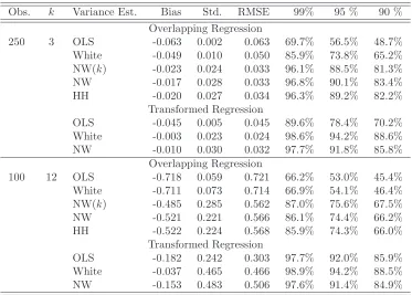
Obs. k Variance Est. Bias Std. RMSE 99% 95 % 90 % Overlapping Regression
250 3 OLS -0.063 0.002 0.063 69.7% 56.5% 48.7% White -0.049 0.010 0.050 85.9% 73.8% 65.2% NW(k) -0.023 0.024 0.033 96.1% 88.5% 81.3% NW -0.017 0.028 0.033 96.8% 90.1% 83.4% HH -0.020 0.027 0.034 96.3% 89.2% 82.2%
Transformed Regression
OLS -0.045 0.005 0.045 89.6% 78.4% 70.2% White -0.003 0.023 0.024 98.6% 94.2% 88.6% NW -0.010 0.030 0.032 97.7% 91.8% 85.8%
Overlapping Regression
100 12 OLS -0.718 0.059 0.721 66.2% 53.0% 45.4% White -0.711 0.073 0.714 66.9% 54.1% 46.4% NW(k) -0.485 0.285 0.562 87.0% 75.6% 67.5% NW -0.521 0.221 0.566 86.1% 74.4% 66.2% HH -0.522 0.224 0.568 85.9% 74.3% 66.0%
Transformed Regression
OLS -0.182 0.242 0.303 97.7% 92.0% 85.9% White -0.037 0.465 0.466 98.9% 94.2% 88.5% NW -0.153 0.483 0.506 97.6% 91.4% 84.9%
Table 2: Monte Carlo simulations: No return predictability. Heteroscedastic error
[image:18.595.116.489.430.697.2]Obs. k Variance Est. Bias Std. RMSE 99% 95 % 90 % Overlapping Regression
250 3 OLS -0.021 0.003 0.021 90.4% 79.2% 70.7% White -0.021 0.004 0.021 89.8% 78.4% 70.0% NW(k) -0.009 0.008 0.012 96.9% 90.5% 83.9% NW -0.006 0.010 0.011 97.5% 91.8% 85.8% HH -0.007 0.010 0.012 97.2% 91.1% 84.8%
Transformed Regression
OLS -0.002 0.006 0.006 98.9% 94.7% 89.4% White -0.002 0.007 0.007 98.7% 94.4% 89.1% NW -0.004 0.010 0.010 98.0% 92.8% 87.1%
Overlapping Regression
100 12 OLS -1.319 0.112 1.323 68.2% 55.4% 47.6% White -1.352 0.116 1.357 64.6% 51.9% 44.3% NW(k) -0.923 0.439 1.022 83.2% 72.7% 65.2% NW -0.973 0.335 1.029 84.4% 73.0% 65.1% HH -0.973 0.340 1.031 84.1% 72.8% 65.0%
Transformed Regression
[image:19.595.117.487.69.336.2]OLS -0.712 0.240 0.751 93.3% 83.5% 75.5% White -0.734 0.281 0.786 92.5% 82.4% 74.3% NW -0.638 0.431 0.770 92.4% 83.0% 75.6%
Table 3: Monte Carlo simulations: Return predictability. Homoscedastic error terms.
For each estimator, the bias in the estimate, its standard error, its root mean square error and true confidence levels of 99%, 95% and 90% are shown.
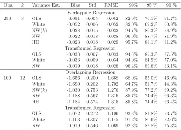
Obs. k Variance Est. Bias Std. RMSE 99% 95 % 90 % Overlapping Regression
250 3 OLS -0.051 0.005 0.052 82.9% 70.1% 61.7% White -0.052 0.006 0.052 82.0% 69.2% 60.8% NW(k) -0.028 0.015 0.032 94.7% 86.3% 78.9% NW -0.022 0.018 0.028 96.0% 88.7% 81.9% HH -0.023 0.018 0.029 95.7% 88.1% 81.2%
Transformed Regression
OLS -0.033 0.007 0.033 94.3% 85.3% 77.5% White -0.033 0.009 0.034 94.0% 84.9% 77.0% NW -0.019 0.018 0.026 96.4% 89.6% 83.1%
Overlapping Regression
100 12 OLS -1.656 0.200 1.668 68.0% 55.0% 46.9% White -1.690 0.202 1.702 64.7% 51.7% 44.3% NW(k) -1.030 0.753 1.276 87.9% 77.2% 69.2% NW -1.188 0.567 1.316 85.7% 74.4% 66.3% HH -1.184 0.574 1.315 85.8% 74.4% 66.4%
Transformed Regression
OLS -1.072 0.272 1.106 92.3% 81.8% 73.7% White -1.103 0.307 1.145 91.2% 80.6% 72.6% NW -0.919 0.546 1.069 92.3% 82.8% 75.3%
Table 4: Monte Carlo simulations: Misspecification. For each estimator, the bias in
[image:19.595.116.489.430.697.2]Table 2 reports results from simulations where the errors are conditionally heteroscedastic.
The presence of heteroscedasticity has a clear effect, significantly worsening the performance
of the OLS covariance estimates obtained from the transformed regression. Here, the White
(heteroscedasticity consistent) covariance estimate obtained from the transformed regression
performs very well and clearly better than the Hansen-Hodrick estimator in the overlapping
regression. The Newey-West estimator applied to the transformed regression is again inferior
to the White estimator, since there is no autocorrelation structure left that may be captured
by the Newey-West estimator.
Table 3 reports results from simulations where the regressors and errors follow the same
pro-cesses as in Table 1, but the actual returns are predictable with a one-period ahead R2- of
20% percent. The results are broadly similar to those in Table 1. Again the procedures based
on the transformed regression perform best, and the best performing estimator is again OLS
applied to the transformed regression. Note however that when returns are predictable, the
OLS covariance estimator applied to the transformed regression is biased down as it ignores
the serial correlation in one-period returns due to the predictability of returns. As in Table
1, the Newey-West estimator applied to the transformed regression is inferior to the OLS
estimator in respect of both noise and bias.
The data generating processes simulated so far have a noise term that is serially
uncorre-lated. Where there is some correlation structure in the noise, our approach should be helpful
in stripping out the autocorrelation induced by the overlapping scheme, making it easier to
account for any remaining underlying autocorrelation in estimating the standard error of the
parameter estimates. A very common cause of autocorrelated noise process is the use of a
misspecified regression model. To examine this case, we rely on the same data generating
The results, in Table 4, confirm our intuition. As in the previous tables, the covariance
estimators from the overlapping regression are severely biased downwards, with the use of
Newey-West and Hansen-Hodrick reducing but not eliminating the bias. The bias and
cover-age ratios are all much worse than in Table 1, the base case, because of the autocorrelation
in the error term. Again, the covariance estimators from the transformed regressions perform
better than ones from the original regressions, but the autocorrelation in the error term
in-duces significant bias in the OLS and White estimators. The biases are reduced by the use
of Newey-West, and the coverage ratios are closer to their nominal levels.
The broad conclusions drawn from these tables seem to be robust to the choice of parameters.
In particular, if the regressors are less persistent (AR parameter of 0.1 rather than 0.8)
simulations (not reported here) also show that the procedures performed on the transformed
regressions work best, with the Newey-West estimator being the best in presence of remaining
autocorrelation, the White estimator being the best in the presence of heteroscedasticity and
the OLS estimate being best otherwise.
4
Review of Two Financial Studies
Overlapping regressions have been central to the debate over the predictability of stock market
returns (Fama & French (1988); Campbell & Shiller (1988)). To illustrate the relevance of
our approach we conduct two analyses using real rather than simulated data. In the first
we re-examine the issue of the predictability of long-horizon US stock market returns using
Robert Shiller’s data on stock market returns and earnings. In the second we illustrate our
approach to Fama-MacBeth regressions by looking at the predictability of relative country
stock returns. Although we introduced our methodology only in the context of plain linear
It should be emphasised that the purpose of this analysis is to illustrate the approach to
overlapping regressions we have developed in this paper rather than to cast new light on
the debate over the predictability of stock prices. In particular, we have not attempted to
allow for other econometric issues raised by the use of a highly persistent regressor, or the
joint endogeneity of the dependent and independent variables. Here, we only show the effect
our methodology in terms of efficiency gains for standard errors under the same assumptions
under which they were originally derived in the literature.
4.1
US Stock Market Predictability
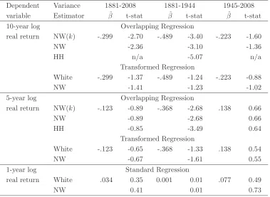
Taking data from Robert Shiller’s website (http://www.econ.yale.edu/ shiller/ data.htm) for
annual US stock returns (S&P 500) and price-earnings ratios from 1871 to 2008, we estimate
the regression
rt,t+k =βrt−k,t+ut+k
wherert,t+k is the k period log real return fromttot+k. The results are set out in Table 5.
Where the dependent variable is the ten-year return (k = 10), the standard approach, with either Newey-West or Hansen-Hodrick estimates of the covariance matrix, leads to severe
underestimates of the standard error, with corresponding over-estimates of the t-statistics,
in comparison to the analysis based on the transformed regression. This bias is observable
also in each of the sub-periods. The coefficient on the lagged return, which appears to be
significantly negative over the whole period and in the first half period, is indistinguishable
from zero when using the transformed regression. For the five year return, the position
is broadly similar except that the coefficient is not significantly different from zero in either
the standard or the transformed regression except when looking at the first half of the period.
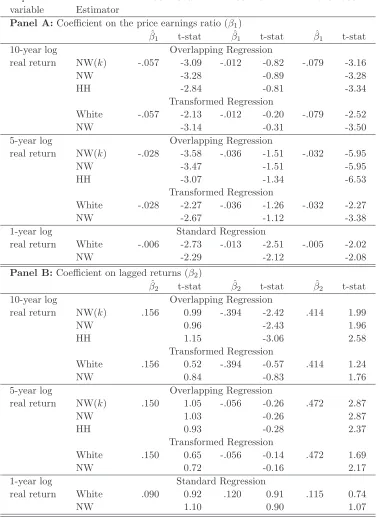
consider the regression
rt,t+k =β1Xt+β2rt−k,t+ut+k
where rt,t+k is the k period log real return from t to t+k and Xt the year t ratio of price
to smoothed earnings. The results are set out in Table 6. The results are similar to the
pre-vious regression in that the standard approach, with either Newey-West or Hansen-Hodrick
estimates of the covariance matrix, leads to severe underestimates of the standard error, with
corresponding over-estimates of the t-statistics, in comparison to the analysis based on the
transformed regression. This bias is observable also in each of the sub-periods. ’n/a’ indicates
cases in which the estimated Hansen-Hodrick covariance matrix is not positive definite. The
coefficient on the price earnings ratio is significantly negative at conventional significance
lev-els both over the period as a whole, and in the second half, under both the standard approach
and the transformed regression, but the standard errors are roughly doubled. This holds true
both for five and ten year rolling returns. The coefficient on lagged returns, which appears
to be significantly positive in the second half of the period for both 5 and 10 year returns,
and to be significantly negative in the first half for 10 year returns, turns out to be
insignifi-cantly different from zero when using the transformed variables. In almost every transformed
regression we observe the tendency that the Newey-West t-statistics are slightly higher than
the White ones, indicating that they are picking up some remaining autocorrelation pattern
Dependent Variance 1881-2008 1881-1944 1945-2008 variable Estimator βˆ t-stat βˆ t-stat βˆ t-stat 10-year log Overlapping Regression
real return NW(k) -.299 -2.70 -.489 -3.40 -.223 -1.60
NW -2.36 -3.10 -1.36
HH n/a -5.07 n/a
Transformed Regression
White -.299 -1.37 -.489 -1.24 -.223 -0.88
NW -1.41 -1.23 -1.02
5-year log Overlapping Regression
real return NW(k) -.123 -0.89 -.368 -2.68 .138 0.66
NW -0.89 -2.68 0.66
HH -0.85 -3.49 0.64
Transformed Regression
White -.123 -0.65 -.368 -1.33 .138 0.54
NW -0.67 -1.61 0.55
1-year log Standard Regression
real return White .034 0.35 0.001 0.01 .077 0.49
[image:24.595.110.489.72.349.2]NW 0.41 0.01 0.73
Table 5: Estimation results for regressionrt,t+k=rt−k,tβ+ut+k, wherert,t+k is thek-year
Dependent Variance 1881-2008 1881-1944 1945-2008 variable Estimator
Panel A:Coefficient on the price earnings ratio (β1)
ˆ
β1 t-stat βˆ1 t-stat βˆ1 t-stat
10-year log Overlapping Regression
real return NW(k) -.057 -3.09 -.012 -0.82 -.079 -3.16
NW -3.28 -0.89 -3.28
HH -2.84 -0.81 -3.34
Transformed Regression
White -.057 -2.13 -.012 -0.20 -.079 -2.52
NW -3.14 -0.31 -3.50
5-year log Overlapping Regression
real return NW(k) -.028 -3.58 -.036 -1.51 -.032 -5.95
NW -3.47 -1.51 -5.95
HH -3.07 -1.34 -6.53
Transformed Regression
White -.028 -2.27 -.036 -1.26 -.032 -2.27
NW -2.67 -1.12 -3.38
1-year log Standard Regression
real return White -.006 -2.73 -.013 -2.51 -.005 -2.02
NW -2.29 -2.12 -2.08
Panel B:Coefficient on lagged returns (β2)
ˆ
β2 t-stat βˆ2 t-stat βˆ2 t-stat
10-year log Overlapping Regression
real return NW(k) .156 0.99 -.394 -2.42 .414 1.99
NW 0.96 -2.43 1.96
HH 1.15 -3.06 2.58
Transformed Regression
White .156 0.52 -.394 -0.57 .414 1.24
NW 0.84 -0.83 1.76
5-year log Overlapping Regression
real return NW(k) .150 1.05 -.056 -0.26 .472 2.87
NW 1.03 -0.26 2.87
HH 0.93 -0.28 2.37
Transformed Regression
White .150 0.65 -.056 -0.14 .472 1.69
NW 0.72 -0.16 2.17
1-year log Standard Regression
real return White .090 0.92 .120 0.91 .115 0.74
[image:25.595.109.487.82.600.2]NW 1.10 0.90 1.07
Table 6: Estimation results for regressionrt,t+k =Xtβ1+rt−k,tβ2+ut+k, wherert,t+k is
4.2
Country Stock Returns
Since our approach can easily be generalized to Fama-MacBeth panel regressions we illustrate
its implications by analyzing return predictability in international equity indices. Richards
(1997) documents reversal in the relative returns of international equity indices. Countries
that have done relatively well in the past period tend to under-perform their peers in the
fu-ture. The reversal is strongest at the three year horizon. The finding is confirmed by Balvers,
Wu & Gilliland (2000).
A natural way of exploring the predictability of relative country returns at different horizons is
to follow the Fama-MacBeth procedure using country stock indices as the assets. Specifically
we run the following cross-sectional regressions for every montht
rt,t+k =rt−k,tβt+ut+k, (12) wherert,t+k is the vector ofk-month returns across different countries from month ttot+k.
We then test whether the estimated slope coefficient differs from 0. Like Richards (1997),
the country returns are the MSCI equity index returns less the return on the US market,
taken from Datastream. The period is January 1982 to May 2007, and the countries are
Austria, Australia, Belgium, Canada, Denmark, Germany, Hong Kong, Ireland, Italy, Japan,
Netherlands, Norway, Singapore, Sweden, Switzerland, and the UK. The results are shown
in Table 7.
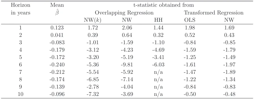
The point estimate of beta is positive at the one year horizon. This is consistent with the
findings of Bhojraj (2006), and suggests some momentum in returns at shorter horizons. The
value of beta goes negative at longer horizons, taking its largest negative values at around
the six year horizon. According to the untransformed regression, the beta is significantly less
than zero for horizons of four years or more (the reason that no Hansen-Hodrick t-statistics
to the transformed regression with simple OLS standard errors, however, the positive beta at
the one year horizon is just significant, but at all other horizons the beta does not significantly
differ from zero. Using Newey-West standard errors in the transformed regression suggests
that no beta is significantly different from zero.
Horizon Mean t-statistic obtained from
in years βˆ Overlapping Regression Transformed Regression
NW(k) NW HH OLS NW
1 0.123 1.72 2.06 1.44 1.98 1.69
2 0.041 0.39 0.64 0.32 0.52 0.43
[image:27.595.79.524.176.349.2]3 -0.083 -1.01 -1.59 -1.10 -0.84 -0.85 4 -0.179 -3.12 -4.23 -4.69 -1.59 -1.79 5 -0.172 -3.20 -5.19 -3.41 -1.25 -1.49 6 -0.240 -5.36 -9.81 -6.03 -1.61 -1.97 7 -0.212 -5.54 -5.92 n/a -1.47 -1.89 8 -0.174 -6.85 -7.14 n/a -1.22 -1.34 9 -0.139 -2.78 -4.04 n/a -0.84 -0.83 10 -0.096 -7.32 -3.69 n/a -0.50 -0.48
Table 7:The table shows the estimate of the regression coefficient of long horizon country index returns
on lagged returns. The basic regression isrt,t+k=rt−k,tβt+ut+k where rt,t+k is the vector ofk-month log returns (in excess of the US log return) across 22 different countries from montht tot+k, and the slope parameter estimates are then pooled and tested for whether the mean (’mean beta’) differs from zero. Since the regressions are done each month, the data are overlapping, so the t-statistics are adjusted for autocorrelation using a Newey-West (NW) or Hansen-Hodrick (HH) procedure. As an alternative the regression is transformed as described in the text and the standard error is calculated from the transformed regression (’transformed regression’). The data are from Datastream.
5
Conclusion
The main contribution of this paper is to introduce a simple transformation of the
regres-sor matrix which turns a long horizon regression with overlapping observations into a short
horizon regression with non-overlapping observations. This transformation greatly simplifies
parameter inference. We show that standard inference techniques such as OLS, White and
Newey-West parameter standard errors can be applied to the transformed regression and
perform better than more sophisticated methods utilized directly with the overlapping
We show, using Monte Carlo studies, that our method dominates conventional techniques
in all three cases of homoscedastic, heteroscedastic and autocorrelated error terms in small
samples. In the cases of homoscedastic and heteroscedastic error terms our method is
asymp-totically equivalent to Hansen-Hodrick type estimators, but when there is residual
autocor-relation (not induced by the overlapping scheme) our method dominates asymptotically as
well as in small samples.
The intuition behind the efficiency gain in our method is that we explicitly account for a
known deterministic aggregation pattern a priori and do not try to estimate it in a noisy
way, as for example through pre-whitening or through Hansen Hodrick or Newey-West type
approaches. The efficiency gain of our method in comparison to methods designed to account
only for the autocorrelation induced by the overlapping scheme (Hansen-Hodrick) is higher the
more autocorrelation structure is present in the error terms of the non-overlapping regression.
In this paper we introduce our methodology in the context of overlapping regressions, but
the methodology is applicable to a wider range of data aggregation schemes, as long as they
are deterministic and known to the researcher.
The importance of using more reliable standard errors have been shown by reviewing two
important empirical studies. The transformation of a long-horizon regression into a
References
Andrews, D. W. K. (1991): “Heteroskedasticity and Autocorrelation Consistent
Covari-ance Matrix Estimation,”Econometrica, 59 (3), 817–58.
Andrews, D. W. K. & J. C. Monahan (1992): “An Improved Heteroskedasticity and
Autocorrelation Consistent Covariance Matrix Estimator,”Econometrica, 60 (4), 953–66.
Ang, A. & G. Bekaert (2007): “Stock Return Predictability: Is it There?” Review of
Financial Studies, 20 (3), 651–707.
Bacchetta, P., E. Mertens, & E. van Wincoop (2009): “Predictability in Financial
Markets: What do Survey Expectations Tell us?” Journal of International Money and
Finance, 28 (3), 406 – 426.
Baker, M., R. Greenwood, & J. Wurgler(2003): “The Maturity of Debt Issues and
Predictable Variation in Bond Returns,”Journal of Financial Economics, 70 (2), 261 –
291.
Balvers, R., Y. Wu, & E. Gilliland (2000): “Mean Reversion across National Stock
Markets and Parametric Contrarian Investment Strategies,”Journal of Finance, 55 (2),
745–772.
Bhojraj, S. (2006): “Macromomentum: Returns Predictability in International Equity
Indices,”Journal of Business, 79 (1), 429–428.
Boudoukh, J., M. Richardson, & R. Whitelaw (2008): “The Myth of Long-Horizon
Predictability,”Review of Financial Studies, 21 (4), 1577–1605.
Campbell, J. Y. & R. J. Shiller (1988): “The Dividend-Price Ratio and Expectations
Campbell, J. Y., A. W. Lo, & A. C. MacKinlay(1997): The Econometrics of Financial
Markets, Princeton University Press.
Cochrane, J. H.(1991): “Volatility Tests and Efficient Markets : A Review Essay,”Journal
of Monetary Economics, 27 (3), 463–485.
Cochrane, J. H. & M. Piazzesi(2005): “Bond Risk Premia,”American Economic Review,
95 (1), 138–160.
Daniel, K. & D. Marshall(1997): “Equity-Premium and Risk-Free-Rate Puzzles at Long
Horizons,”Macroeconomic Dynamics, 1 (02), 452–484.
Evans, M. D. & R. K. Lyons(2005): “Meese-Rogoff Redux: Micro-Based Exchange-Rate
Forecasting,”American Economic Review, 95, 405–414.
Fama, E. F. & K. R. French (1988): “Dividend Yields and Expected Stock Returns,”
Journal of Financial Economics, 22 (1), 3–25.
Gregory Mankiw, N. & M. D. Shapiro (1986): “Do we Reject too Often? : Small
Sample Properties of Tests of Rational Expectations Models,”Economics Letters, 20 (2),
139–145.
Hansen, L. P. & R. J. Hodrick(1980): “Forward Exchange Rates as Optimal Predictors
of Future Spot Rates: An Econometric Analysis,”Journal of Political Economy, 88 (5),
829–53.
Hjalmarsson, E.(2006): “New Methods for Inference in Long-Run Predictive Regressions,”
International Finance Discussion Papers 853, Board of Governors of the Federal Reserve
System (U.S.).
Hodrick, R. J. (1992): “Dividend Yields and Expected Stock Returns: Alternative
Jagannathan, R. & Y. Wang(2005): “Consumption Risk and the Cost of Equity Capital,”
NBER Working Papers 11026, National Bureau of Economic Research.
—— (2007): “Lazy Investors, Discretionary Consumption, and the Cross-Section of Stock
Returns,”Journal of Finance, 62 (4), 1623–1661.
Jegadeesh, N.(1991): “Seasonality in Stock Price Mean Reversion: Evidence from the U.S.
and the U.K,”Journal of Finance, 46 (4), 1427–44.
Lamont, O. (1998): “Earnings and Expected Returns,” The Journal of Finance, 53 (5),
1563–1587.
Lettau, M. & S. Ludvigson (2001): “Consumption, Aggregate Wealth, and Expected
Stock Returns,”The Journal of Finance, 56 (3), 815–849.
Malloy, C., T. Moskowitz, & A. Vissing-Jorgensen(2005): “Consumption Risk and
the Cost of Equity Capital,” Working paper, GSB, University of Chicago.
Nelson, C. R. & M. J. Kim(1993): “Predictable Stock Returns: The Role of Small Sample
Bias,”Journal of Finance, 48 (2), 641–61.
Newey, W. K. & K. D. West (1987): “A Simple, Positive Semi-Definite,
Heteroskedas-ticity and Autocorrelation Consistent Covariance Matrix,”Econometrica, 55, 703–708.
Parker, J. (2001): “The Consumption Risk of the Stock Market,” Brookings Papers on
Economic Activity, 2, 179–348.
Parker, J. A. & C. Julliard (2005): “Consumption Risk and the Cross Section of
Ex-pected Returns,”Journal of Political Economy, 113 (1), 185–222.
Richards, A. J. (1997): “Winner-Loser Reversals in National Stock Market Indices: Can
Richardson, M. & T. Smith (1991): “Tests of Financial Models in the Presence of
Over-lapping Observations,”Review of Financial Studies, 4 (2), 227–54.
Stambaugh, R. F. (1999): “Predictive Regressions,” Journal of Financial Economics,
54 (3), 375–421.
Sul, D., P. C. B. Phillips, & C.-Y. Choi (2005): “Prewhitening Bias in HAC
Estima-tion,”Oxford Bulletin of Economics and Statistics, 67 (4), 517–546.
Valkanov, R. (2003): “Long-horizon Regressions: Theoretical Results and Applications,”
Journal of Financial Economics, 68 (2), 201–232.
White, H. (1980): “A Heteroskedasticity-Consistent Covariance Matrix Estimator and a
Direct Test for Heteroskedasticity,”Econometrica, 48 (4), 817–38.