Some topics in homogenization

(1)

University of Warwick institutional repository: http://go.warwick.ac.uk/wrap

A Thesis Submitted for the Degree of PhD at the University of Warwick

http://go.warwick.ac.uk/wrap/34600

This thesis is made available online and is protected by original copyright. Please scroll down to view the document itself.

(2)

Some topics in homogenization

by

Charles Manson

Thesis

Submitted to the University of Warwick

in partial fulfilment of the requirements

for admission to the degree of

Doctor of Philosophy

Mathematics Institute

(3)

Acknowledgments

Thanks for to my mother and brother for all their love and support. Thanks to my

supervisor, Martin Hairer for his help and encouragement. In addition I would

like to thank Warwick University for financial support via a Warwick Postgraduate

(7)

Declarations

(8)

Abstract

This thesis is mainly concerned with solving a new type of periodic

homogeniza-tion problem. A soluhomogeniza-tion of removing the Diophantine hypothesis on the

homog-enization problem where the interface sits at an irrational angle to the period is

attempted but is not yet complete. As an aside an oscillator problem is analyzed

(9)

Abbreviations

We will use the following notation,

R the real numbers,

N the natural numbers,

Td _the_d_{dimensional torus,}

B a Brownian motion,

(10)

Chapter 1 Foreword

The aim of this thesis is to extend existing results on periodic homogenization.

Fully periodic homogenization was initially investigated in the late 70s by

Ben-soussan, Lions and Papanicolaou [BLP78] and since then a large number of

varia-tions on the theme have emerged as have many applicavaria-tions in a diverse range of

fields. There are a number of standard techniques which have led to the study of

properties of solutions to certain PDEs, such as the solution to the Poisson

equa-tion, studied extensively in a series of papers. This particular equation is useful in

the production of a ”corrector term”, which will be explained fully in due course.

Initially, the assumptions were quite rigid, such as the diffusion coefficient was

assumed to be uniformly elliptic, and full periodicity was enforced, then ellipticity

was relaxed to hypoellipticity. Then recently in a paper by my supervisor and

Par-doux [HP08], the uniformly elliptic and hypoellipticity assumption was relaxed

al-lowing the diffusion matrix to vanish even on an open set. There are myriad other

ways in which the assumptions have been changed, or the techniques adapted to

new fields such as materials science since the seminal book [BLP78].

There are a number of papers that relax the periodicity in one set of spatial

vari-ables and average over the periodic fast varivari-ables to produce a diffusion with

”ho-mogenized” coefficients, that is, coefficients derived from the original coefficients,

(11)

quan-tity with respect to the invariant measure (on the torus) of the fast process.

Period-icity can also be relaxed with respect to the consideration of a reflected diffusion

process (the solution to an SDE involving a local time term). These two approaches

are even combined such as by Diakhaby and Ouknine in [DO06].

We allow two periodic regions where the drift is centered and periodic in each

region with a thickened hyperplane interface region in between these two periodic

regions. To show the weak convergence in one dimension to a rescaled skew

Brow-nian motion with a different scaling factor on either side of the interface, which

upon homogenization, has now reduced to a point (this only happens in one

di-mension, in general the interface becomes a hyperplane), we use a scheme first

employed by Freidlin and Wentzell [FW93] to perform averaging on a graph.

The end result in homogenization is weak convergence in the space of

probabil-ity distributions on a suitably chosen space, usually the space of continuous paths

or cadlag paths (right continuous paths with left hand limits). This is usually

achieved via a three or four step process of first showing ”tightness” and then

identifying the limit point, either by showing resolvent convergence or using the

tool of the martingale problem by showing that the solution must then satisfy a

particular martingale problem. If the martingale approach is utilized, then there

is the extra step of showing that the solution of the martingale problem is unique.

The final step, and a step not always taken or not relevant in some cases, is

charac-terizing the diffusion process corresponding to a particular resolvent or particular

martingale problem. This thesis does not deviate from the standard approach in

taking these steps when performing homogenization and we use the martingale

problem approach.

Chapter 2 is an introduction to the field in general, the main problem to be solved,

and techniques required to solve it. The subsequent chapter 3 is the proof of the

result in one dimension. Chapter 4 is the main result, the multidimensional result,

which is followed by an attempt to homogenize in the reflected periodic setting

(12)

final chapter 6 we study a homogenization inspired approach to a coupled

(13)

Chapter 2 Introduction

2.1 The machinery of homogenization

There are several important concepts that perhaps should be explained before we

proceed. At this point it is probably foremost to bear in mind that in

homogeniza-tion, through the variation of a parameter (such as ε above), the object of study

becomes a collection of probability distributions on an appropriate space, usually

the space of continuous or cadlag functions from an interval of R to a suitably

”nice” metric space. (In our case the space is that of continuous functions from

[0,∞) toRd.) We will now embark on a quick review of the background theory

to homogenization, the language of stochastic differential equations, semigroups

and such like. The first formal concept to be introduced, therefore, is tightness of a

family of probability distributions, establishment of which is usually the first step

in a typical probabilistic homogenization proof.

Definition 2.1.1(Tightness for a family of probability measures [Bil99]).

A family of probability measures, on a metric space (S,d), {Pi}I ⊆ P(S) (P(S)

the set of probability measures on S), for an arbitrary (possibly uncountable)

in-dexing set, is tight, if givenε >0, there exists a compact setK ⊆Ssuch that,

inf

i∈IPi(K) ≥1−ε.

This is then combined, when (S,d) is complete and separable, with

Pro-horov’s theorem. ProPro-horov’s theorem gives the equivalence of tightness and

(14)

nature of the Prohorov metric is not important in this context, just that in the case

Sis separable, convergence in the Prohorv metric is equivalent to (in a general

met-ric space this reduces to implies) weak convergence of probability measures [EK86,

Theorem 3.1 Chapter 3]. It is weak convergence that is the sought after property in

a lot of homogenization proofs and this is defined as follows,

Definition 2.1.2(Weak convergence [Bil99]).

Given a metric space (S,d), let Cb be the space of bounded continuous functions

with the supremum norm. A sequence{Pn}n converges weakly toP∈ P(S), if

lim n→∞

Z

f dPn =

Z

f dP, ∀f ∈ Cb(S).

Therefore, by showing tightness in a complete and separable metric space

and applying the Prohorov theorem we have that any subsequence from our

orig-inal collection of probability measures has a weakly convergent subsequence. The

tightness of the family of measures is usually shown on the space C([0,∞),Rd)

with the topology of uniform convergence on compact sets.

The second step is then to show that any weak limit of the family of probability

distributions either satisfies a particular martingale problem or possesses a

partic-ular resolvent. It is probably prudent at this point to define both these quantities.

Definition 2.1.3(Martingale problem).

The definition of the solution to a martingale problem according to [EK86] is as

follows.

Let B(S) denote bounded measurable real-valued functions on the metric space

S. Then given an operatorL : B(S) →B(S), a solution of the martingale problem

forLis a measurable stochastic processXdefined on a probability space(Ω,F,P)

with values in Ssuch that for f, g ∈ B(S) with f ∈ D(L) (f in the domain of L)

and g=Lf, we have that

f(X(t))−

Z t

0 g(X(s))ds,

is a martingale with respect to the filtration

?_FX

t =FtX∨σ

Z s

0 h(X(u)) : s

≤t, h∈ B(S)

(15)

for F_tX = σ(X(s) : s ≤ t), for a right continuous process ?F_tX = F_tX and in

general the difference between the two consists only of null sets.

Since we are dealing with martingale problems in spaces of continuous paths

we have ?F_tX = F_tX and hence the distinction between?F_tX and F_tXis ignored

from now on.

The concept of a resolvent belongs to the study of strongly continuous

semi-groups, so it is logical to define the resolvent in this setting and then to move onto

how this definition relates to the particular situation of homogenization of the

so-lutions to SDEs.

Definition 2.1.4(Strongly continuous semigroup [EK86]).

A one parameter family {S(t) : t ≥ 0} of bounded linear operators on a Banach

space Bis called a semigroup if S(0) = I and S(t+s) = S(t)S(s)for alls, t ≥ 0.

A semigroup{S(t)}onBis said to be strongly continuous if limt→0S(t)f = f, for

every f ∈ B.

The infinitesimal generator of a semigroup {S(t)} on B is the linear operator A

defined by

A f =lim t→0

1 t

S(t)f − f.

The domainD(A)ofAis the subspace of all f ∈ Bfor which the above limit exists.

It can be shown that the generator of a strongly continuous semigroup is

closed, i.e. that the graph of the generator, considered as a subset of B×B, is

closed, and thatD(A)is dense, see for instance [EK86, Corollary 1.6 Chapter 1].

Definition 2.1.5(Resolvent [EK86]).

Given a closed operator Aon the Banach spaceB, if, for a realλ, λI−A :=λ−A

is one-to-one, has a range equal to Band (λ−A)−1is a bounded linear operator

on B, then λ is said to belong to the resolvent set of A and the bounded linear

operator(λ−A)−1is called the resolvent of A.

In the particular case of an SDE with suitably nice coefficients (Lipschitz

(16)

as a Markov process. The semigroup on a closed subspace M⊆ B(S) correspond-ing to a Markov process is that given by,

E

f(X(t+s))|F_tX = EX(t)

f(X(s)) =

Z

SP(s,X(t),dy)f(y),

for all f ∈ M, and whereP(s,X(t),dy)is the measure corresponding to the Markov

transition kernel.

Where the Markov process is the solution of an SDE onRd, in order to obtain

the generator we look to It ˆo’s formula and take the expectation. For a real valued

C2(twice continuously differentiable) function, f onRn, we have, from a repeated

application of stochastic integration by parts followed by approximation argument

[RY91], It ˆo’s formula:

f(X(t)) =

Z t

0 ∂2f ∂xi∂xj

(X(s))dhXi,Xji(s) +

Z t

0 ∂f ∂xi

(X(s))dXi(s),

(2.1.1)

where the convention of summation over repeated indices (Einstein summation

convention as it’s otherwise known), is assumed to hold.

This finishes a brief introduction to the language of homogenization, in the

next section we will move onto a review of some classic homogenization problems.

2.2 A Classic Problem

In this section we will begin to show how homogenization techniques are

imple-mented in practice. We will begin with a classic problem that was solved in the

early days in the book [BLP78].

Let Bbe a standard Wiener process and in the classic problem it is assumed

that b : Rn → Rn_{, smooth, and periodic. In the homogenization problems we}

will study later,b : Rn → Rn_{, smooth, is periodic away from an ’interface’ region}

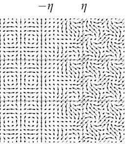
[−η,η], η ≥ 0. More precisely, we will assume that there exist periodic functions

bi : R →R,i =±, such thatbi(x+1) = bi(x)and such thatb(x) = b+(x−η)for

x > η and b(x) = b−(x+η) for x < −η. We study the solution of the stochastic

differential equation (SDE),

dX

dt =b(X(t)) + dB

(17)

in particular the weak convergence of the solution under a diffusive rescaling. This

SDE has a unique solution up to indistinguishability as the coefficientsband 1 are

Lipschitz [RY91, Theorem 2.1 Chapter IX]. Two processesY,Y0defined on the same

probability spaceΩ are indistinguishable if for almost allω ∈ Ω, Yt(ω) = Y_t0(ω)

for allt[RY91].

A diffusive rescaling is given by x 7→ εx and t 7→ ε2t, exactly the ratio of

pow-ers that preserves the Brownian motion component of the motion. This rescaling

gives the behavior of the process over large distances and large times. Applying

the aforementioned rescaling, what is really the object of study is the family of

solutions of the SDEs indexed byε,

dXε x dt =

1

εb

Xε x

ε

+dB

dt , Xε

x(0) = x. (2.2.1)

The above rescaled equation is arrived at by ignoring the initial condition and

considering the integrated form of the standard equation, given by, for,

X(t) =

Z t

0 b(Xx(s))ds+B(t) ,

setting,

Xε(_t) =

εX

t

ε2

.

We use the normal change of variables formula to exchangetfor t

ε2 in the integral

with respect todton the RHS, i.e. set ”new”sequalsε2times ”old”sin the integrals

and then end up with the rescaled equation except withεB

t ε2

as the second term

on the RHS,

Xε(_t) =

Z t

0

1

εb

Xε x(s)

ε

ds+εB

t

ε2

. (2.2.2)

As mentioned in passing above though, this term is another Brownian motion

courtesy of Levy’s characterization theorem [RY91], which states,

(18)

is an Ft-Brownian motion; (ii) X is a continuous local martingale andhXi,Xjit = δi jt for every 1 ≤ i, j ≤ d; (iii) X is a continuous local martingale and for every d-uple

f = (f1, . . . ,fd)of functions in L2(R+), the process

Eti j =exp

i

∑

k

Z t

0 fk(s)dX k s +

1

2

∑

_k

Z t

0 f 2 k(s)ds

,

is a complex martingale.

(Whereh·,·idenotes quadratic variation.)

So using parts (i) and (ii) of Levy’s characterization theorem, for the processεB(ε−2t),

this is, by definition ofB,F_ε−2_tadapted (notice the change of filtration), vanishes at

zero, continuous, and hashεB(ε−2t),εB(ε−2t)i = ε2hB(ε−2t),B(ε−2t)i = ε2ε−2t =

t. Therefore it is anF_ε−2_t Brownian motion.

In addition, in order for the scaling limit of the SDE (2.2.1) that we will consider, to

exist, we require thatb(or each of the two functionsbi, glued together to makeb),

satisfy a centering condition. The centering condition prevents the process from,

intuitively speaking, ”running off to infinity” by exhibiting an increasing overall

drift in a particular direction as the parameterεis reduced to zero. This condition

is used in the classic, fully periodic case to ensure existence of a weak limit (the

concept of a weak limit will be explained below, in the next section). The fact that

a weak limit exists [BLP78] with the centering condition implies that violation of

this condition results in a process that exhibits an increasing overall drift.

Explic-itly, the centering condition onbiis given by,

Z 1

0 bi(x)pi(x)dx=0 ,

where pi denotes the density of the invariant measure for the solution to the SDE

dX

dt =bi(X) + dB

dt , (2.2.3)

fori =±, considered as a diffusion on the torus, which satisfies the Fokker Planck

equation,

(19)

forLthe generator of (2.2.3) given byb∂x+ (1/2)∂2_xandL?its adjoint in a suitable

space (the Sobolev space H1 for instance) given by L?φ = −∂x(bφ) + (1/2)∂2xφ.

See [BLP78] for a proof of the existence of the density of the invariant measure as

the unique solution of the Fokker Planck equation using the Fredholm alternative.

If X(t) is the solution to the SDE onRd given by the integral equations for

i =1,. . . ,d,

Xi(t) = Xi(0) + r

∑

j=1

Z t

0 gi j X(s)

dBj(s) +

Z t

0 hi X(s)

ds,

for g and h measurable functions taking values in the d×r matrices and d

di-mensional vectors respectively, and the Bj are r standard independent Brownian

motions. Then applying It ˆo’s formula gives, for f ∈C2, a real valued function,

f(X(t)) =

Z t

0 ∂2f ∂xi∂xj

(X(s))gi k X(s)

gj k X(s)

ds

+Z t

0 ∂f ∂xi

(X(s))hi X(s)

ds

+Z t

0 ∂f ∂xi

(X(s))

∑

j

gi j X(s)

dBj(s)

.

Looking at the RHS of the above expression, observe the semimartingale structure

evident from the grouping of terms, the first two terms are of bounded variation

and the last term, by the martingale property of the It ˆo integral, is a martingale.

Hence, if the solution of the SDE were considered as a Markov process then the

generator would be given by gi kgj k ∂

2

∂xi∂xj +hi

∂

∂xi. Not all solutions to SDEs are

Markov Processes but under basic assumptions, such as g and h Lipschitz, we

have that the solution is a Markov Process, in fact with Lipschitz coefficients the

solution is a Feller process [RY91, Theorem 2.5 Chapter IX].

Now we have introduced It ˆo’s formula, we will show how it is used to define a

corrector term that facilitates homogenization in a simple case, by considering the

corrected process instead of the original process which is ”close” to the original

process but with a much nicer form of generator. The corrected process takes the

form, Xε+

εg(ε−1Xε), and what we aim to do with the additional term is remove

(20)

we are in the case of wholly periodic drift. In other words for the purposes of

the following discussion we will assume that b is fully periodic and satisfies the

centering condition. An application of It ˆo’s formula then gives the appropriate

g, in particular it shows that this is the case if g satisfies the Poisson equation for

b, Lg = −b, componentwise. Note that we will frequently denote the generator

of the semigroup corresponding to the solution of an SDE by L, and in this case

L =b.5+5.5. Applying It ˆo’s formula to Xε

x+εg(ε−1Xε)gives, Xε

x(t) = x+εg

x

ε

+Z t

0

1

εb

Xε x(s)

ε

ds+B(t)

+Z t

0

1

εbi

Xε x(s)

ε

∂g ∂xi

Xε x(s)

ε

ds

+Z t

0

1 2ε

∑

_i

∂2g ∂xi∂xi

Xε x(s)

ε

ds

+Z t

0 ∂g ∂xi

Xε x

ε

dBi(s)−εg

Xε

ε

,

where Bidenotes the components of theddimensional Brownian motion B. Thus

ifLg=−b, whereL =bi(x)_∂∂_x_i +1₂4is the generator of the non-rescaled process,

then the above equation becomes,

Xε

x(t) +εg

Xε

ε

= x+εg

x

ε

+B(t) +

Z t

0 ∂g ∂xi

Xε x(s)

ε

dBi(s)

= x+εg

x

ε

+Z t

0

∑

_i

1+ ∂g

∂xi

Xε x(s)

ε

dBi(s) .

(2.2.4)

Notice that the term of order ε−1 is now gone. With one extra lemma, 2.2.3, we

can finish the homogenization of this equation using the martingale central limit

theorem [EK86] which is as follows,

Theorem 2.2.2(Martingale Central Limit Theorem). For n=1,2,. . ., n, let(F_tn)be a filtration and let Mn be anF_tn-local martingale with sample paths in D_Rd[0,∞)(space

of cadlag paths) and Mn(0) = 0. Let Ai jn be a symmetric d×d matrix-valued process such that Ai jn has sample paths in DR[0,∞)and An(t)−An(s) is non-negative definite for t>s ≥0. Assume one of the following conditions holds:

(i) For each T >0,

lim n→∞E

sup t≤T

|Mn(t)−Mn(t−)|

(21)

and

Ai jn =hMin,M j ni .

(ii) For each T >0and i, j=1, 2,. . ., d, lim

n→∞E

sup t≤T

|Ai jn(t)−Ai jn(t−)|

=0 ,

lim n→∞E

sup t≤T

|Mn(t)−Mn(t−)|2

=0 ,

and for i, j =1,2,. . ., d,

Mi_n(t)Mnj(t)−Ai j(t),

is anFn-local martingale.

Suppose that C = ci j is a continuous, symmetric, d×d matrix-valued function, defined on[0,∞), satisfying C(0) =0and

∑

i j

ci j(t)−ci j(s)

ξiξj ≥0 ξ ∈ Rd, t>s ≥0 ,

and in addition, we have that for each t ≥0and i, j = 1, 2,. . ., d Ai jn(t) →ci j(t) ,

in probability. Then Mn ⇒ X, where X is the process with independent Gaussian incre-ments and covariance ci j(t). (The existence of which is ensured by [EK86, Theorem 1.1 Chapter 7].)

The lemma in question, remembering we are still in the fully periodic case

for the purposes of this discussion, is (see for example [BMP07, Proposition 2.4]),

Lemma 2.2.3. Let f ∈ L∞(Td,R), then for any t >0, we have the following convergence in probability,

Z t

0 f

Xε(_s)

ε

ds →t

Z

Td f(x)µ(dx) ,

(22)

The proof of this lemma is very similar to a lemma in the one dimensional

case of the problem we will be studying, so to avoid repetition, will be omitted.

Looking at the form of the RHS of (2.2.4) it is quite clear how we will apply the

martingale central limit theorem. Since the paths of the stochastic integral are

con-tinuous, both conditions (i) and (ii) from the martingale central limit theorem are

satisfied and we will use the lemma above to show convergence in probability of

the quadratic variation of the stochastic integral. The quadratic variation of the

stochastic integral on the RHS of (2.2.4) is given by,

Z t

0

∑

_k

1+ ∂gi

∂xk

Xε

ε

dBk(s),

Z t

0

∑

_k

1+ ∂gj

∂xk

Xε

ε

dBk(s)

=t

Z

Td

∑

k

1+ ∂gi

∂xk

Xε(_s)

ε

1+ ∂gj

∂xk

Xε(_s)

ε

ds .

Lemma 2.2.3 then gives the convergence in probability of the quadratic variation

to,

Z t

0

∑

_k

1+ ∂gi

∂xk

Xε(_s)

ε

1+ ∂gj

∂xk

Xε(_s)

ε

ds

→t

Z

Td

∑

k

1+ ∂gi

∂xk

(x)

1+ ∂gj

∂xk

(x)

µ(dx) = ci j(t) ,

and then the martingale central limit theorem gives the weak convergence of the

stochastic integral term to the process with independent Gaussian increments given

by ci j(t), which by an application of the Levy characterization theorem quoted

above componentwise, is a Brownian motion with a homogenized diffusion

coeffi-cient in front of it. Then once it has been noted that addition of the termεg(ε−1Xεx)

(using the Wasserstein metric) does not affect the weak limit, we have the weak

convergence of the process to the aforementioned limit.

To see that the addition of the termεg(ε−1Xε)and in fact any term that is bounded

above by a term that tends to zero as ε → 0 does not affect weak convergence

we will use the Wasserstein metric [Vil03]. This metrizes weak convergence on a

Polish space of bounded diameter, which is whatC([0,∞),Rd)is; uniform

(23)

by,

D(ω,ω0) =

∞

∑

n=1

1 2n

sup₀_≤_t_≤_n|ω(t)−ω0(t)|

1+sup₀_≤_t_≤_n|ω(t)−ω0(t)| .

This then gives that the corrected process will tend to the same weak limit as the

uncorrected process which is the rationale behind correcting in this fashion. The

Wasserstein metric is defined as follows,

Definition 2.2.4(Wasserstein Metric).

The Wasserstein metric is defined by, forµ1, µ2measures on a spaceΩ, the

corre-sponding distance between them is given by,

inf

(µ1,µ2)∈Γ

Z

|x1−x2|d(µ1,µ2),

where Γ is the set of all couplings of the measures µ1 and µ2. That is measures

on Ω×Ωthat have projection onto the first component µ1, and onto the second

component,µ2.

Consider the family of couplings indexed by εgiven by the push forward

onto C([0,∞),Rd)×C([0,∞),Rd) of µ1, the law of Xxε, by the map x 7→ (x,x+

εg(ε−1x)). The convergence of the two families of measures given by the corrected

and non-corrected processes to the same limit, considered as probability measures

on the spaceC([0,∞),Rd), is seen by taking this family of couplings indexed byε.

Then the Wasserstein distance between the limiting point of the family of corrected

processes and the distribution of the non-corrected process asε→0 is less than,

Z

D

x1,x1+εg

x1 ε

dµ1 ≤ εkgk∞ ,

which tends to zero as ε →0. Hence the measures given by the processes

consid-ered as probability measures on the spaceC([0,∞),Rd), converge weakly asε→0.

This is known as periodic homogenization, albeit a simple case, and the manner of

usage of the corrector term is similar to that used for the problems to be solved in

this thesis. In the next subsection we will introduce the slightly more complicated

(24)

theory, and this will be the starting point for a review of some of the research into

this theory.

The ”toy” example of the last subsection was a simplification of the

prob-lems investigated in fully periodic homogenization probprob-lems. The SDE to be

ho-mogenized usually has an extra drift term and the diffusion term is no longer a

constant equal to the identity. Such an SDE would for example be given by, in

integrated form,

Xε

x(t) =x+

Z t

0

1

εb

Xε x(s)

ε

ds+

Z t

0 c

Xε x(s)

ε

ds+

Z t

0 σ

Xε x(s)

ε

dB(s),

whereb,c : Rd →Rd_{are smooth vector valued functions and}

σ: Rd→Rd×Rdis

a smooth matrix valued function. Note that because of the extra term in the drift,

this equation does not come from a rescaling as the more simple example of the

previous chapter did. Without the extra drift term it would correspond again to a

rescaling.

In addition to an extra term and additional complexity of the diffusion term, there

is also in many homogenization problems the consideration of fast and slow

vari-ables. An example of this is known as locally periodic homogenization. In the case

of locally periodic homogenization where there are both fast and slow variables,

the drift is for example,

ε−1b(Xε_x(s),ε−1X_xε(s)) .

The variable Xε

x(s) is termed the slow variable whereas the variable ε−1Xεx(s) is

the fast variable. Obviously they are related, but the terminology comes from the

general strategy used to tackle such problems, namely treat the slow and fast

vari-ables as independent varivari-ables, and through the use of correctors and bounding

inequalities for the results, contrive a situation where averaging with respect to

the fast variables can be conducted. The full SDE in a typical locally periodic

ho-mogenization problem is of the form,

Xε

x(t) = x+

Z t

0

1

εb X

ε

x(s),ε−1Xεx(s)

+

c Xε

x(s),ε−1Xεx(s)

ds

+Z t

0 σ X

ε

x,ε−1Xεx(s)

(25)

Apart from the ”standard” assumptions of boundedness and differentiability with

bounded derivatives on the coefficients, the hypotheses on the drift in this case are

that, for fixed x, b(x,y) is periodic inyand centered, andc(x,y), σ(x,y) are

peri-odic iny. The regularity assumptions are made to avoid too many technical details

that detract from a presentation of the overall scheme. The concept of centering in

this situation clearly differs slightly from that considered above since the process

is no longer a diffusion on the torus. The operator Lx,y on R2d, obtained as the

generator of the diffusion process given in (2.2.5), except pretending the fast and

slow variables are now distinct spatial variables, for fixed x, is the generator of a

diffusion process onRd that can be considered as the generator of a diffusion

pro-cess on the torus. For fixed x, the driftb(x,y) is centered with respect tom(x,dy)

the invariant measure of the aforementioned diffusion on the torus. In what

fol-lows we assume smoothness to investigate the general principles and avoid a lot

of the details that arise when regularity assumptions are much looser. For example

in [BLP78] the coefficients are assumed to be, for the second variable fixed, twice

continuously differentiable in the first variable but in [BMP07] this assumption is

relaxed and although the basic structure of the proof is the same, the latter is

sig-nificantly heavier in technical detail.

In both of these cases, the use of a corrector term does not completely remove

the drift, but it does remove the term of order ε−1 from the equation and the

re-maining terms can be homogenized by a similar lemma to that used to show the

convergence in probability of the quadratic variation term in the simple case. We

will first deal with the simpler situation of periodic homogenization with the extra

drift termcas in [BLP78], then move onto outlining how a locally periodic

homog-enization result would proceed. Applying It ˆo’s formula to Xε

x(t) +εg(ε−1Xεx(t))

(the corrector term which we refer to as gis also commonly referred to as ˆb),

Xε

x(t) +εg

Xε x(t)

ε

=x+εg

x

ε

+Z t

0 (I+

5g)c

Xε x(s)

ε

ds

+Z t

0 (I+

5g)σ

Xε x(s)

ε

dW(s) ,

(26)

demonstrate weak convergence of, we have an additional integral term of bounded

variation. Remembering how convergence in probability of the quadratic variation

of the stochastic integral term was achieved, using the lemma (2.2.3) that gave

the convergence in probability of the quadratic variation term, we therefore also

have convergence in probability of the integral with respect tods. Convergence in

probability implies weak convergence, hence this lemma gives,

Z t

0 (I+5g)c

Xε x(s)

ε

ds⇒t

Z

Td(I+5g)c(y)µ(dy).

Therefore putting all parts together, we have the weak convergence ofXε

x(t)to the limit,

x+t

Z

Td(I+5g)c(y)µ(dy) +Z

Td(I+5g)σσ

T₍_I₊_5g₎T₍_y₎

µ(dy)

1₂

dB˜s,

where the exponent of the homogenized quadratic variation term denotes the unique

symmetricd×dmatrix that when composed with its transpose will give this

quan-tity and ˜Bdenotes addimensional Brownian motion.

Moving on now to locally periodic homogenization as in [BLP78]. This is far

more complicated than the cases considered previously due to the presence of the

process to be homogenized as an order 1 input term in the drift and diffusion

coef-ficients. Instead of just using a corrector and showing convergence in probability

of the SDE termwise, the procedure of homogenization at least on a general level

is more akin to the method we will employ. First tightness for the family of

proba-bility distributions onC([0,∞),Rd)is shown and then the limit point is identified.

This is a departure from the method of homogenization employed in the previous

simpler case. Originally in the proof of the simpler homogenization results

out-lined above in [BLP78], the proof did have a verification of tightness followed by

an argument to identify the limit, following the same general method as we will

outline in the case of locally periodic homogenization. Practically speaking,

tight-ness of the family{Pε_}

εis often shown by verifying that the following conditions

hold, firstly that, givenT <∞,η >0,

lim δ&0sup_ε P

ε

sup t2−t1<δ, 0≤t1<t2≤T

|x(t2)−x(t1)| <η

(27)

where we denote the evaluation map by x(·). The second condition is that, lim

M→∞sup_ε P ε

x(0) ≥M =

0 .

The first of these is basically asserting the existence of a uniform modulus of

con-tinuity over the whole family in a probabilistic sense. The second condition is a

measure of the uniform occupation by the initial conditions of a compact set, in

a probabilistic sense. This second condition in much of the homogenization that

will be outlined is trivial since we are seeking to demonstrate weak convergence of

the family of solutions (viewed as probability distributions) starting from the same

initial point. Therefore we only have to verify the first of these conditions with the

supremum over ε replaced by lim sup_ε→₀. In order to do this, a corrector term is

used, in fact the same one as above but with an additional slow component, call

the corrector gagain, which is therefore a smooth periodic vector-valued function

satisfying,

Lx,yg(x,y) = −b(x,y),

Z

Tdg(x,y)µ(x,dy) =0 .

WhereLx,yis the differential operator inygiven by,

Lx,y =bi(x,y) ∂

∂yi

+1

2ai,j(x,y)

∂2

∂yi∂yj ,

andm(x,dy)is the invariant measure of the process generated on the torus byLx,y.

We then apply It ˆo’s formula as standard toXε

x+εg(Xεx,ε−1Xεx), to give, fora=σσT as is common notation,

Xε

x(t) +εg

Xε x(t),

Xε x(t)

ε

=x+εg

x, x

ε

+Z t

0

1

εb+c ds

+Z t

0 σdB(s) + Z t

0 (∇xg+

1

ε∇yg)b ds

+Z t

0 (ε∇xg+∇yg)c ds+ Z t

0 (ε∇xg+∇yg)σdB(s)

+Z t

0

h

εtr(aHx(g)) + 1

εtr(aHy(g))

+tr a(∇x∇yg+∇y∇xg)

i

(28)

Where Hx(g) and Hy(g) are the matrices of second order derivatives of g with

respect toxandyrespectively. Now, the terms of order 1_ε cancel since Lx,yg=−b.

In fact in [BLP78] they show tightness for the non-corrected process by adding

the corrector term and its expansion from the It ˆo formula on the same side of the

equality. In keeping with the what follows we have done the opposite. Now, to

verify tightness we look at sup_|_t₁₋_t₂_|<δ|Xε

x(t1)−Xxε(t2)|. Since the integrands in

the expression above with respect to ds are bounded due to the assumption of

bounded derivatives, for |t1−t2| < δ, andε < 1, these integrals are bounded by

C1δ. Since the only other non-fixed quantities are the stochastic integral terms. The

integrand in the quadratic variation of the stochastic integral term (collecting them

into one term) is bounded forε < 1, byCsay, hence the quadratic variation up to

time T is bounded by CT. Then to produce the same type of inequality as that

produced in [BLP78], we use Chebychev’s inequality which is frequently used in

bounding arguments on the stochastic integral term and note the bounds on the

integrals of bounded variation. Chebychev’s inequality is as follows,

Definition 2.2.5(Chebychev’s Inequality).

For any positive random variableYandk >0, we have that,

P[Y >k] ≤ E[Y] k .

There are many forms of this inequality, but this is the one we will use most

frequently and is very general in its formulation.

So using this inequality, and denoting the stochastic integral term byS(t), we have

that, forδsufficiently small,

Ph sup

|t1−t2|<δ,t1,t2<T

|Xε

x(t1)−Xεx(t2)| ≥ η

i

≤Ph sup |t1−t2|<δ,t1,t2<T

|S(t1)−S(t2)| ≥η−C1δ

i

=Ph sup |t1−t2|<δ,t1,t2<T

|S(t1)−S(t2)|2 ≥(η−C1δ)2

i

≤ CTδ

(29)

Where Chebychev’s inequality is used in the last inequality. We then clearly have,

lim

δ&0lim sup_ε→₀ P

h

sup t2−t1<δ, 0≤t1<t2≤T

|Xε

x(t2)−Xεx(t1)| ≥ η

i

=0 ,

and hence tightness.

So now the second (and last) stage in a large number of homogenization

proofs, but usually the most difficult, is identifying any limit point of the

fam-ily of probability measure as one particular probability measure for all

conver-gent subsequences. The rationale behind this is as follows, by Prohorov’s theorem,

tightness is equivalent to weak relative compactness, i.e. for any subsequence of

measures in a tight family of probability measures, there is a further subsequence

that converges weakly to a probability measure. Thus, if it is possible to identify

the limit of any convergent subsequence as a particular measure then this must

be the limit point of any subsequence and therefore the unique limit point of the

entire family. In a proof of locally periodic homogenization or in fact any

homog-enization, a common type of lemma to see is the following where L2convergence

is commonly substituted for convergence in probability as in the corresponding

result for fully periodic homogenization investigated earlier, or even convergence

in a Sobolev space. This is because as the diffusion part of the limiting process is

no longer Gaussian but a variable stochastic integral with respect to a Gaussian

process (Brownian motion) so we are no longer using the Martingale Central Limit

Theorem and instead just showing the convergence of the appropriate conditional

expectations for which we only need L1 convergence. The stochastic part of the

limiting process is no longer a Gaussian since the dependence of the diffusion

co-efficient on the slow variable remains.

Lemma 2.2.6. Let h(x,y)be a function which is C2in x, C1in y, with all partial deriva-tives continuous and bounded globally in x, y. Suppose also that h is periodic in y for fixed x and satisfies,

Z

Td h(x,y)µ(x,dy) =0 , ∀x.

Then we have that,

E

Z t

s h

Xε(_u)_, X ε(_u)

ε

du

2

Fs

(30)

Proof. The following method of proof is quite common for showing such conver-gence. Take the periodic solution of

Lx,yh˜ =h. Then we apply It ˆo’s formula to,

ε2h˜

Xε(_t)_, X ε(_t)

ε

−ε2h˜

Xε(_s)_, X ε(_s)

ε

=Z t

s (ε∇x ˜

h+∇yh˜)b ds+

Z t

s (ε 2_∇

xh˜+ε∇yh˜)c ds

+Z t

s (ε 2_∇

xh˜+ε∇yh˜)σdB(s)

+Z t

s ε

2_tr₍_aH

x(h˜)) +tr(aHy(h˜)) +εtr a(∇x∇yh˜ +∇y∇xh˜)ds .

Upon doing so, we then note that the only constant order terms areLx,yh˜ =h. For

bounded t,s, the rest of the integral terms multiplied by εto some positive power

are bounded thus we have,

E

Z t

s h

Xε(_u)_, X ε(_u)

ε du 2 Fs

= (O(ε) +O(ε2))2 =O(ε2)

Thus showing the required L2convergence.

The next step in identifying the limit is to adopt the same approach as [BLP78]

and use the tool of the martingale problem mentioned above with the corrected

process. Denote Xε

x(t) +εg(Xεx(t),ε−1Xxε(t)) by Zε(s) for ease of notation. Let

φ ∈ C∞₀ (Rd)(the space of smooth real valued functions onRd with compact

sup-port), and using It ˆo’s formula with the semimartingale expression for the corrected

process derived by It ˆo’s formula above gives forφ(Zε),

φ Zε(s)+ Z t

s

∇xφ Zε(s)

c+∇xg b+ε∇xg c+∇yg c

+εtr(aHx(g)) +tr(a(∇x∇yg+∇y∇xg))

du

+Z t

s

∇xφ(Zε(s))

σ+∇ygσ+ε∇xgσ

dB(u)

+Z t

s tr

H(φ) (σ+∇ygσ+ε∇xgσ)(σ+∇ygσ+ε∇xgσ)Tdu.

Now we introduce the averaged coefficients (vector-valued and matrix-valued,

(31)

that will be coefficients of the generator of the weak limit point of the family to be

homogenized,

r(x) =

Z

Tdc(x,y) +∇xg(x,y)b(x,y)

+∇yg(x,y)c(x,y) +2tr(a(x,y)∇x∇yg(x,y))µ(dy)

=Z

Tdr(x,y)µ(dy),

q(x) =

Z

Td(I+∇yg(x,y))a(x,y)(I+∇yg(x,y))

T

µ(dy)

=Z

Tdq(x,y)µ(dy),

for r(x,y) and q(x,y) the two integrands. So what we do now is take φ(Xεx(s) +

εg(Xε_x(s),ε−1Xε_x(s)))and subtract the generator of the process given by r(x) and

q(x) above applied to φ and take conditional expectation of both sides, apply

Lemma 2.2.6 and then take expectation of both sides. Since all derivatives are

bounded we can make the substitution of Xε(_t) _for _Zε(_t) _{in all the terms of finite}

variation at a cost ofKεin total, for some constantK,

Ex

φ(Xε(t))−φ(Xε(s))− Z t

s

∇φr(Xε(u))du

−

Z t

s H(φ)q(X

ε(_u))_du

Fs

=Ex

Z t

s ∇φ r(X ε(_u)_,

ε−1Xε(u))−r(Xε(u))du

+Z t

s H(φ). q(X ε(_u)_,

ε−1Xε(u))−q(Xε(u))du+K0ε

Fs

(2.2.7)

since all the stochastic integral terms vanish after taking conditional expectation

with respect toFs(which is traditionally what stochastic integral terms of the form

Rt

s . . . dM(u), forMa martingale, do when expectation with respect toFsis taken

under appropriate bounding assumptions). Taking the expectation of the modulus

of both sides of (2.2.7) and then using the Cauchy Schwarz inequality together with

(2.2.6) and Jensen’s inequality on the right hand side gives that the left hand side

tends to zero in L1 as ε → 0. We have convergence of probability distributions

weakly at least along a subsequence. Thus, taking the limit of (2.2.7) along such

(32)

which gives that any limiting measure in the sense of weak convergence is the

solution to the martingale problem given by the operator ¯L,

¯

L =r(x).∇+q(x).∇∇ (2.2.8)

It is at this point that things get slightly more complicated than the previous

ex-ample since we no longer have the martingale central limit theorem to do all the

work for us. Although we now know that any weak limit point of the family of

measure indexed byεmust satisfy the martingale problem given by (2.2.8), we do

not know that the solution to this martingale problem started from a particular

point is unique. In other words we still do not know that the family of probability

measures converges to any specific measure as yet. If we could show that there is

only one solution to the martingale problem given a particular initial point then

we would have done just that. Looking at the form of the limiting solution of the

martingale problem given in (2.2.8) it is clear to see this is of the same form as

martingale problems solved by the solutions to SDEs and a theorem from [SV69]

is used to show uniqueness of the solutions to such martingale problems

corre-sponding to the solution of SDEs.

2.3 Associated benefits of homogenizing SDEs

The probabilistic homogenization of an SDE leads to homogenization in an

ap-propriate sense of the Dirichlet problem. For instance in conducting the locally

periodic homogenization discussed above, Bensoussan, Lions and Papanicolaou

[BLP78] were not just studying homogenization of SDEs as a problem in itself,

once you have homogenized an SDE like the one just previously, you get for free

the limiting solution to the set of Dirichlet problems, for continuous f,

−a_ijx, x

ε

_∂uε

∂xij −1

εbi

x, x

ε

_∂uε

∂xi

−cx, x

ε

_∂uε

∂xi

+a0

x, x

ε

uε = f(x), f|_Γ ≡0 ,

as ε → 0. The Dirichlet problem is considered in a domain O with boundary Γ,

(33)

connection between the SDE and the solution to the Dirichlet problem is given by

the explicit formula for the solution to the Dirichlet problem,

Ex

Z τ_Oε

0 f(X

ε(_t))_exp

−

Z t

0 a0

Xε(_s)_,X ε(_s)

ε ds dt , (2.3.1)

where τ_Oε is the escape time from the domain O by the process Xε. Then as a

result of the weak convergence of the laws of the stochastic differential equations

corresponding to Xε _{we have} _uε(_x) _→ _u(_x) _{for all}_x _∈ O _as

ε → 0 where u(x)is

the solution to the Dirichlet problem,

−qij(x) ∂u

∂xij

−ri(x)∂u

∂xi

+a¯0(x)u= f(x), f|Γ ≡0,

for,

¯

a0(x) = Z

Tda(x,y)µ(x,dy),

The problem term in the expression (2.3.1) is the order ε−1 argument of a0 in the

expression (2.3.1), since the most obvious route to the convergence is to apply the

weak convergence that has just been outlined to get the pointwise convergence of

solutions. We get round this by swappinga0for its averaged version and

demon-strating that the cost of doing so tends to zero asε→0. We have,

Ex

Z τ_Oε

0 f(X

ε(_t))_exp

−

Z t

0 a0

Xε(_s)_, X ε(_s)

ε ds dt

−Ex

Z τ_Oε

0 f(X

ε(_t))_exp

−

Z t

0 a¯0(X

ε(_s))_ds

dt

≤CEx

Z ∞ 0 exp − Z t

0 a0

Xε(_s)_, X ε(_s)

ε ds −exp − Z t

0 a¯0(X

ε(_s))_ds

dt ,

forCbounding the supremum norm of f on O. With the hypothesis of strict

pos-itivity on a0, we have the convergence of the RHS of this expression to zero by

Lemma 2.2.6. By the positivity ofa0, the second term on the LHS of the above

ex-pression is a continuous bounded function on the space of continuous paths, hence

tends to, by weak convergence ofXε

x,

Ex

Z _τε

O

0 f(

¯

X(t))exp

−

Z t

0 a¯0(

¯

X(s))ds

dt

,

denoting the solution to the martingale problem corresponding to the differential

(34)

2.4 Homogenization in random media

The remaining large field in probabilistic homogenization is known as

homoge-nization in random media. It can be briefly summarized as follows. A particularly

accessible introduction can be found in [Oll94]. The original, seminal text in this

field is by Papanicolaou and Varadhan [PV81].

For homogenization in random media the typical set up [Rho09a] is that

we have a random medium given by a probability space(Ω,G,µ)and a group of

measure preserving{τx : x ∈Rd}transformations acting ergodically onΩ:

• ∀A∈ G,x ∈Rd_,

µ(τx(A)) =µ(A),

• If for anyx ∈ Rd_,

τx(A) = A, thenµ(A) = 1 or 0,

• For any measurable functiongon (Ω,G,µ), the function(x,ω) → g(τxω)is

a measurable function on(Rd×Ω,B(Rd₎_{× G}₎_.

Then there are a number of different avenues to explore in terms of how this

trans-lates into a homogenization problem, the classic case is explored in [PV81], given

by the diffusion corresponding to the martingale problem with uniformly elliptic

operator,

1

2∂i(a(τ−xεω)∂j) .

Although most of this paper is approaching the problem from the direction of the

convergence of the corresponding PDE. An example of another quite classic

prob-lem can be found in [Oll94], where the probprob-lem under consideration is that of the

homogenization of SDEs of the form,

X(t) =

Z t

0

−DV(τ−X(s)(ω))ds+W . (2.4.1)

W is a Brownian motion independent of the random medium and V : Ω → Ris

a random potential, andDV(ω)is then defined as the differential inxof the

func-tion x 7→ V(τ−x(ω)). It is assumed that V and DV are bounded and in addition,

stochastic continuity can be shown from the properties of the random medium

(35)

Remark 2.4.1. In private communication with R´emi Rhodes it was brought to my attention that the three properties of the random medium given above, by a proof

constructed by himself and F. Delarue, together imply stochastic continuity,

Definition2.4.2 (Stochastic continuity). ForThf(ω) = f(τ−hω), lim

h→0µ(|Thf(ω)− f(ω)| ≥ δ) = 0, ∀δ >0, f ∈ L 2₍

µ)

Stochastic continuity is used to give density of the domain of the

infinitesi-mal generator D, ofTx inL2(µ) from [EK86, Corollary 1.1.6] as the generator of a

strongly continuous semigroup. Ultimately the density of the domain is used to

show convergence of the resolvent equation via the spectral theorem that will be

our surrogate corrector in the random environment case. We will make this precise

shortly.

Under these hypotheses, as one would expect, the question is that of the

weak convergence ofεX(ε−2t)asε→0.

An extension of the classic problem explored in this article [Oll94] is that of

a particle moving in a free divergence random field,

X(t) =

Z t

0 F(τX(s)ω)ds+W(t),

forWas above and F =D.Hfor all anti-symmetric matrix H. In the case of a free

divergence random field there is no longer reversibility to simplify the analysis

slightly, as there is in the case of (2.4.1), as far as the weak convergence ofεX(ε−2t).

Extending this scenario in the manner in which periodic homogenization

was extended, results in situations akin to those explored above for periodic

ho-mogenization. Such homogenization problems have been explored in a number

of papers by Rhodes. In [Rho09a], the locally periodic homogenization mentioned

previously is extended to the random medium case. We have a family of SDEs of

the form,

Xε(_t) =_x+

Z t

0 b

ω,X

ε(_s)

ε ,X

ε(_s)

ds+

Z t

0 c

ω, X

ε(_s)

ε ,X

ε(_s)

ds

+Z t

0 σ

ω,X

ε(_s)

ε ,X

ε(_s)

dB(s) ,

for B as above and ω from the random medium again. In addition we have

(36)

of the standard form f(ω,x,y) = f(τyω,x). The assumption of uniform ellipticity

(ΛI ≤ σσ ≤ Λ−1I for some Λ > 0) of the diffusion coefficient is made together

with ability of the generator ofX to be written in divergence form (for the matrix

a+H, asymmetric, H antisymmetric in this case) and regularity assumptions on

the coefficients. The potentially degenerate case is dealt with in another paper by

Rhodes, [Rho09b]. The uniform ellipticity is used to provide local ergodicity of

the process and also to provide uniform (over the random environment)

(Aron-son type) estimates on the density to give tightness. Lack of uniform ellipticity

in [Rho09b] with regard to local ergodicity is countered with weak local

ergodic-ity assumptions which are enforced through a reference matrix which controls the

degeneracies of the diffusion coefficient.

Then in [Rho09c], we have a corresponding homogenization problem for a

reflected diffusion process,

Xε(_t) =

Z t

0 b(τX

ε(_s)(ω))ds+

Z t

0 σ(τX

ε(_s)(ω))dB(s)

+Z t

0 γ(τX

ε(_s)(ω))dL(t)ε,

where the situation is as before except Lε _{is the local time of} _Xε(_t) _and

γ1 = 1 as

is required for a reflected diffusion process and the matrix that is used to give the

generator of the process in divergence form is symmetric this time. The

restric-tions on the coefficients are so made to enable certain calcularestric-tions to be carried out

regarding the auxiliary problems mentioned below.

Reflecting for a minute on the generic method one must employ to

success-fully carry out the proof of homogenization, it becomes apparent that the

tradi-tional notion of a corrector is no longer applicable since we do not have an

af-firmative answer to the existence of a corrector with boundedness or sufficiently

slow growth properties. In every classical type random medium homogenization

problem we have a result of the form,

Proposition 2.4.3. The solution to the resolvent equation (componentwise inRd),

(λI−L)ui_λ =bi ,

has the property, for someζ ∈ L2(µ),

(37)

where the subscript 2 denotes the L2norm with respect toµ.

This is used to compensate for the lack of a corrector in the traditional sense

and is the corresponding auxiliary problem in this type of homogenization. It still

retains the philosophy of a corrector though since it is used to cancel highly

oscil-latory terms at the expense of introducing convergent quantities. Although in one

version of the proof presented in [PV81] this result is not taken to hold strongly.

Another possible issue that cannot be resolved as in the periodic case is

com-pactness in the space of continuous paths. This is because in the random case

generically we want tightness over the random medium as well as over the family

of diffusion processes in some sense (tightness of the annealed law), this is either

arrived at as in [PV81, Rho09a] where we obtain tightness on the space of

con-tinuous paths for the family of measures given by Pε_{, for all} _x _{in a compact set,}

ω,

Pε(_F) =

Z

F(ζ(·))Qεx(dζ,ω(·)),

for Fa real valued function on path space and Qε

x(·,ω)the measure on the space

of paths induced byXε

xwithω as the realization of the random environment. The

tightness with respect to the family of annealed laws ¯Pε =

µ(dω)×λ(dx)Pε for

a suitable measure on Rd, λ(dx), can also be obtained directly, see for instance

[Rho09c, Rho09b]. One method of achieving this is using the

Garsia-Rodemich-Rumsey inequality via the Feynman Kac formula to show tightness directly as in

[Oll94] and [Rho09c]. Another alternative is to make estimates on the density using

Nash’s estimates [PV81] or Aronson estimates [Rho09a] to obtain bounds above on

the density that are uniform over the random environment to obtain tightness as

in [PV81].

After obtaining tightness and a result akin to that of Proposition 2.4.3, the

homogenization can then be achieved directly through bounding error terms (in

the PDE framework) [PV81]. Alternatively it is achieved using an ergodic result

(or existence of an ergodic invariant measure [Oll94]) to obtain convergence of the

coefficients/quadratic variation to their averaged form, analogous to those used

(38)

(dependent on the situation in question), this type of result is usually something

similar to,

lim ε→0

¯

Eε x

sup

0≤t≤T

Z t

0 Ψ(X

ε(_s)_,

τ_Xε(_s)/_ε(ω))−Ψ¯(Xε(s))ds

=0 , (2.4.3)

where ¯Eε

xdenotes expectation with respect to the measure ¯Pεi.e. the annealed

ver-sion ofPε_{and ¯}Ψ(_·) =R

Ψ(·,ω)µ(dω). Then proceeding as before except working

in a suitable (annealed) L2 space and using the limit of the ”corrector” as λ = ε2

tends to zero i.e. using the properties of both terms in (2.4.2). This is a slight

over-simplification of the more complicated cases, for instance in [Rho09c] there is a

local time term that must be dealt with. This means that also required are ergodic

results for local time integrals of the form corresponding to that in (2.4.3), tightness

of the local time terms Lε _{and in addition after identifying the limit ¯}_L_{, it is}

neces-sary to show that ¯Lis the local time of the limiting process. This follows from the

fact that ¯Lcan be shown to be associated to the Skorohod problem of the limiting

process and that we have uniqueness in law for the solution of the corresponding

Skorohod problem [LS84] which has a local time solution. By saying ¯Lis associated

to the Skorohod problem of the limiting process ¯Xwe mean that it is an increasing

process and its points of increase are contained within the set{_X¯ ₌₀}. In [Rho09a]

there is the problem of the dependence of the solution to the resolvent equation on

the slow variable which emerges through the difficulty in dealing with the term

b∂yuε2 necessitating an addition ergodic result, Theorem 6.3.

Hopefully the above (brief) summary of homogenization in a random

en-vironment serves to illustrate the prevalence of corrector based approaches even

when there is no existence of correctors in the tradition sense, and additionally to

emphasize the breadth of homogenization literature.

This completes a review of the most accessible and classic cases of

proba-bilistic homogenization. It is at this point that we take stock of non-probaproba-bilistic

methods to analyze the convergence of solutions in the simplest cases such as the

(39)

2.5 Multiscale methods for the homogenization of SDEs

This section is a quick summary of the method of multiscale expansions which is

often applied to similar homogenization problems to the ones we will be dealing

with. For a more detailed exposition of this section see the book by Pavliotis and

Stuart, Multiscale Methods [PS08].

Here instead of a corrector we have the solution to the cell problem that

features prominently and occupies the corresponding position in the method. If

we work through the problem we wish to solve given by (2.2.1) in the fully

peri-odic case again from this perspective and see how the probabilistic methodology

is mirrored in terms of the corrector function by the cell problem. There are a wide

range of different forms of problems that the multiscale expansion method can be

applied to; multiscale expansions is an analytical PDE method that can be applied

to many different classes of PDEs not just those that correspond to SDEs. We will

outline the breadth of the scope of the method of multiscale expansions in due

course. The hypotheses are once again, that the drift b is fully periodic and

cen-tered over the whole ofRdand hence we can consider the process as a process on

Td_for

ε =1. In the multiscale method setting the problem is recast from (2.2.1) to

homogenization of the Cauchy problem,

∂tuε(x,t) =

∆

2 +

b(ε−1x)

ε .5

uε(_x_,_t)_,

uε(_x_{, 0}) = _f(_x)_, _x _∈ Rd_, _(2.5.1)

for f ∈ C₀∞(Rd). This corresponds to the equation satisfied by Ex[f(Xε(t))], for

the SDE with drift ε−1b(ε−1·) and diffusion coefficient 1 on Rd. Using the

rig-orous mathematical background in [PS08], we have the convergence of the

solu-tions to (2.5.1) in L∞(Rd×(0,T)). This is sufficient after verifying tightness in

C([0,∞),Rd) for weak convergence since then convergence of Ex[f(Xε(t))] (the

finite dimensional distributions) in L∞(Rd×(0,T)) implies that the weak limit is

unique.

The basic methodology behind a multiscale expansion is to split the process

into two scales, a slow, macroscopic scale given byx and a fast, microscopic scale

Some topics in homogenization

Some topics in homogenization

Charles Manson

Thesis

Doctor of Philosophy

Mathematics Institute

Contents

Acknowledgments

Declarations

Abstract

Abbreviations

Chapter 1

Foreword

Chapter 2

Introduction

2.1

The machinery of homogenization

2.2

A Classic Problem

∑

∑

∑

∑

∑

∑

∑

∑

∑

∑

∑

∑

∑

2.3

Associated benefits of homogenizing SDEs

2.4

Homogenization in random media

2.5

Multiscale methods for the homogenization of SDEs