An analysis of processor resource models for use in performance prediction

Original citation:

Papaefstathiou, E., Kerbyson, D. J., Nudd, G. R. and Atherton, T. J. (1994) An analysis of processor resource models for use in performance prediction. University of Warwick. Department of Computer Science. (Department of Computer Science Research Report). (Unpublished) CS-RR-279

Permanent WRAP url:

http://wrap.warwick.ac.uk/60952

Copyright and reuse:

The Warwick Research Archive Portal (WRAP) makes this work by researchers of the University of Warwick available open access under the following conditions. Copyright © and all moral rights to the version of the paper presented here belong to the individual author(s) and/or other copyright owners. To the extent reasonable and practicable the material made available in WRAP has been checked for eligibility before being made available.

Copies of full items can be used for personal research or study, educational, or not-for-profit purposes without prior permission or charge. Provided that the authors, title and full bibliographic details are credited, a hyperlink and/or URL is given for the original metadata page and the content is not changed in any way.

A note on versions:

The version presented in WRAP is the published version or, version of record, and may be cited as it appears here.For more information, please contact the WRAP Team at:

An Analysis of Processor Resource Models for Use

in Performance Prediction

E. Papaefstathiou, D.J. Kerbyson, G.R. Nudd, T.J. Atherton

Parallel Systems Group, Department of Computer Science, University of Warwick, Coventry, UK

Abstract

With the increasing sophistication of both software and hardware systems, methodologies to analyse and predict system performance is a topic of vital interest. This is particularly true for parallel systems where there is currently a wide choice of both architectural and parallelisation options; and where the costs are likely to be high. Performance data is vital to a diffuse range of users including; system developers, application programmers and tuning experts. However, the level of sophistication and accuracy required by each of these users is substantially different.

In this paper characterisation based technique is described (considering both application and hardware resources) which addresses these issues directly. Initially, a framework is described for characterisation based approaches. A classification scheme is used to illustrate differences in the level of sophistication and detail in which the underlying resource models are specified. Finally, verification is provided of the characterisation techniques applied to several application kernels on a MIMD system. The performance predictions and error bounds resulting from the level of resource specification are also discussed.

1. Introduction

Performance evaluation is an active area of interest especially within the parallel systems community [18, 26, 34]. It is of interest to all parties involved including machine manufactures, algorithm designers, application developers, application users, and performance analysts. Performance evaluation strategies have been proposed and utilised to allow analysis to take place at various stages of application code development. Prediction techniques can be used to produce performance estimates in advance of porting code. For fine tuning of performance after implementation, monitoring information can be gathered to analyse where performance has effectively been lost when compared with idealised system performance.

Characterisation includes a multitude of techniques for the description of the underlying operations. These range from high-level descriptions, such as a complexity style analysis, down to a detailed low-level description of the analysis of the instruction stream within a processor. The level of detail at which the system is characterised effects the accuracy of the resulting models. In addition the accessibility to system components effects the characterisation that can be performed, e.g. the instruction stream cannot be analysed without having a compiler available which in turn needs access to source code.

Substantial analysis has been carried out for traditional workload characterisation which are used in capacity planning and performance tuning studies [14, 21, 8]. Workload characterisation can only be performed when all components of the system are in place, and thus all measurements can be obtained. However, in the case of the characterisation of parallel systems most performance studies are required before all the system components are available, or before porting codes to individual systems. The characterisation techniques considered in the scope of this work can be used when not all the system components are in place, thus forming predictive characterisation techniques.

There has been little work to date that has provided comparative studies of the different predictive characterisation methods. Further, no classification of the different characterisation methods is in common use. The work presented here aims to overcome this shortfall by suggesting a classification scheme for characterisation techniques, and also to provide comparisons between the characterisation methods. The results presented here show that the level of detail used within the characterisation models substantially effect the accuracy of performance predictions.

In the analysis that is presented here a characterisation framework for parallel systems has been used. This framework consists of separate characterisation of the software, the hardware, and the parallelisation aspects. This framework has been used to a number of performance studies [28, 30, 43]. The analysis that is performed here concentrates on the different characterisation models that can be used for the functional elements of the processors.

In Section 2 the characterisation framework is described. The different characterisation models in common use and a taxonomy for their classification is presented in Section 3. In Section 4 several application kernels are described along with the description of the characterisation models for a distributed memory MIMD system. Predicted and measured results for several characterisation models are given in Section 5 and also analysed to show the prediction error statistics of the different techniques.

Sub-Task Layer

Parallel Template

Hardware Layer Application Layer

Performance Predictions Software

Execution Graphs

Parallelisation Strategy

Communication Structure

Resource Model

Communication Model

2. Characterisation Framework

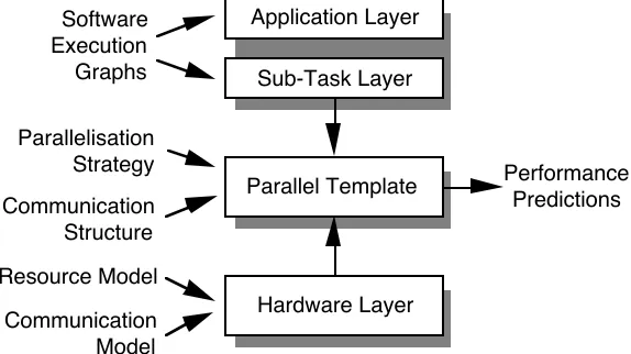
A framework in which characterisation studies can be performed for parallel systems has been proposed and also applied in several studies [28, 30, 43]. This framework consists of several layers, each encompassing different aspects of parallel systems. The four layers contained within this framework as shown in Figure 1. These are:

• An Application layer, which describes the control flow of an application in terms of a sequence of sub-tasks using the software execution graph notation (taken from Software Performance Engineering [38]).

• An Application task layer which describes the sequential part of every sub-task.

• A parallel template layer which describes the parallelisation strategy and communication structure for each task in the application layer.

• A hardware layer which describes the hardware characteristics including CPU, communication operation, and I/O subsystems etc.

The framework has been designed to be modular, such that a parallel template may be interchanged for a given application task. Similarly, the hardware model may be changed to represent a different architecture. This modularity enables characterisation models for each of the parallel templates and hardware resource models to be developed and re-used in further characterisation studies.

Application Stages

Parallelisation Strategies

Hardware Models

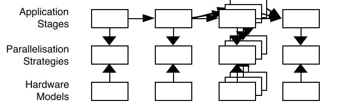
Figure 2 - Schematic example of application tasks with associated parallel templates and hardware models

An example of the use of the layered characterisation framework is shown schematically in Figure 2. Here the application is shown as a sequence of tasks which can either be a set of functions within an application code, or a threaded control sequence through a number of computational kernels (this is the approach being taken within the ESPRIT PEPS characterisation work [29]). For each of the application tasks, a separate parallel template can be used for mapping the task onto a target architecture, and similarly a separate hardware model may be used for each task. It should be noted that the hardware model may be different for each application task (having different resource models for the same hardware), or, as in the case of heterogeneous environments, be hardware models that represent different parallel systems perhaps interconnected through high speed networks such as HiPPi [15].

in Figure 3. Here, a resource model that describes the hardware is chosen, and the associated RUV needs to be obtained for each application component.

Application Stage

Parallel Template

Hardware Layer Resource Usage

Vectors (RUV's)

Resource Models

Resource 1 Resource 2 Resource 3

Figure 3 - Resource models and associated RUV's within the characterisation framework

The RUV for each application component is combined with the resource model, to give predicted execution times for each task, and further the timing information for all task can be combined.

An expression can be developed which captures the control flow of an application. Evaluation of such expressions can provide performance indications for each software component. These expressions are commonly referred to as either time formulas [10], cost functions [2], or performance formulas [16]. Within this paper the term timing formulas will be used. Timing formulas contain both parameters that depend on the nature of data, and also on the resource usage of the system. The data dependent parameters might include loop iteration counts and branch probabilities.

A commonly used method for obtaining timing formulas for complex software structures is the development of control flow graphs [1, 5, 7, 37]. These graphs are often referred to as computation structure models [36], control flow graphs, application abstraction models [31], or software execution graphs [38]. Each node of the graph includes both data dependent parameters and resource usage information. By using graph analysis algorithms, a timing formula can be obtained from it.

max = arr[0]

max=arr[i] max<arr[i]

Nelement

True

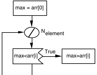
Figure 4 - Software execution graph describing the Find_Max code segment

In this paper Software Execution Graphs (SEG), introduced by Software Performance Engineering, are used [38]. An example of a software execution graph for a serial maximum finding procedure is shown in Figure 4. Computational segments are shown as rectangles, loops as circles with a diagonal line, and conditional branches as a rectangle with a corrugated edge.

t_x =t

(

)

(

( )

( )

(

)

)

where v_assign, v_loop, and v_if are the RUVs for each component of the software execution graph, and the function, t(), takes the specific RUV as a parameter which it expands in terms of the resource model to provide execution time predictions. The number of loop iterations (N_element) and the probability of finding the maximum value (P_max) are data dependent parameters (dependent on the size of the array and the distribution of data).

There are a number of different ways, corresponding to different levels of complexity, in which the resource usage information can be described. This description is coupled with the resource model used for the hardware, and is the subject of the next section.

3. Resource Models within Characterisation Studies

The characterisation techniques in common use involves a description of the software and uses an underlying resource model. The techniques range from high level descriptions, dealing with only a few resource descriptors, through to a detailed micro-analysis concerning an instruction level micro-analysis. The characterisation techniques described are as follows:

• Design Based Characterisation (DBC) - undertaken before software implementation

• Principal Operation Characterisation (POC) - a macro-analysis technique considering only principal operations

• High Level Language Characterisation (HLLC) - a micro-analysis considering constructs within a programming language

• Intermediate Code Characterisation (IntCC) - considers the intermediate code as output by a compiler

• Instruction Code Characterisation (ICC) - examines the actual assembly code that executes on the target system

• Component Timing (CT) - uses actual measurements of the software obtained from a monitoring tool running on the target system

The different resource models contained in the above characterisation techniques are described and compared in this section. Two classification schemes for the different types of the resource models are first introduced below. The important features of the resource models are identified and a detailed examination is given for those contained in the above characterisation techniques.

3.1 Classification of resource models

3.1.1Classification based on the detail of the resource model

The techniques to obtain RUVs have been classified by Cohen [10] into two main categories based on the number and size of operations measured (or predicted):

1.ּ Macro Analysis: These techniques focus on the dominant operations in an algorithm. An example of a macro type analysis is to consider floating point operations while ignoring all others.

2. Micro Analysis: Micro analysis include the techniques that measure all the operations that are performed in a program. This includes a range of techniques from a high level characterisation to a low level instruction characterisation.

3.1.2 Classification based on access to software/system

A further way in which to classify the resource models is based on the access to software/hardware components, e.g. if software is unavailable, or if it is available but a parallel port has not yet been performed. Using this as a basis for classification, the following categories can be used:

1. Abstract Characterisation: This category includes the characterisation methods that can be used in the initial stages of the software development by analysing the algorithms (or designs) being considered.

2. Software Based Characterisation: The methods in this category require the existence of the software source code, and resource usage information which is hardware independent.

3. System Based Characterisation: Finally the characterisation techniques that are system dependent (i.e. both software and hardware dependent) are contained in this category. These methods are used mainly in capacity planning and tuning style performance studies that require high accuracy on a given system.

The two classification schemes described above are complementary, and as such, a particular method may be placed in a category of both classification schemes without overlap. That is, the resource model may be dependent upon available software, but is also considered as a micro-analysis.

3.2 Resource model attributes

The selection of the appropriate resource model for a performance study is dependent on a number of requirements including: the prediction accuracy; the effort required to obtain the RUVs; the status and availability of software; the access to the target system and compiler; and also in the portability of the resource models. These attributes are as follows:

1. System Component Accessibility : Factors that influence the selection of the resource model are the availability of the source code, the compiler, and the hardware system. For example in some cases, the source code may be available, but a compiler and the hardware system are unavailable. Consequently, it would not be possible to measure the performance of each part of the software execution graph using actual measured timing information, or to analyse the output of the compiler.

Finally in post-development stages where tuning and capacity planning is required, actual timing information can be obtained.

3. Portability: A number of resource models are applicable to many hardware platforms while others are specific to a single system.

4. Accuracy: The resultant accuracy, required from the predictions of a characterisation study is another criteria for selecting the appropriate resource model. High accuracy of the results often requires more effort in obtaining the RUVs, and also may be less portable.

5. Effort: The effort involved in obtaining the RUVs is a further factor which should be considered. Typically when low effort is spent the descriptors are either system dependent or the prediction results will be of poor accuracy while high effort may result with high accuracy or high portability. It should be noted however, that obtaining resource usage information can be automated in many cases.

3.3 Description of resource models

The characterisation techniques are placed within the two classification schemes proposed earlier and their properties, according to the list above, are described. Each technique and the associated resource model is described below.

3.3.1Design based characterisation (DBC)

Design based characterisation is performed in the initial stages of software development when source code does not yet exist. The output of this characterisation technique is similar to the RUVs as in the high level language characterisation and the instruction level characterisation described below. However, the procedure used to obtain the RUVs is not based on the analysis of the source code, and the resulting accuracy is substantially different.

Software Performance Engineering suggests an engineering based methodology that allows early performance predictions of a software system, termed performance walkthroughts [38]. The purpose of this technique is to develop the software execution graph of the application, define representative workloads, and estimate the RUV information for each software component. To obtain the RUVs a performance engineer make estimates based on previous experience. The descriptors in SPE studies are presented in terms of CPU execution time, number of I/O calls, number of system calls etc. [37, 38].

Other techniques and tools exist that allow development of control flow graphs in the initial stages of software development including GQUE [22], and QNAP2 [41]. A tool that allows the user to develop computational structure models and define resource usage descriptors in terms of principal high level language operators has also been developed [1].

Design based characterisation conforms to the abstract and macro classifications discussed earlier. Since the characterisation is performed in the early stages of software development, the resulting predictions typically have a low accuracy.

3.3.2 Principal operation characterisation (POC)

possible to make initial predictions of the performance, by identifying the principal operations.

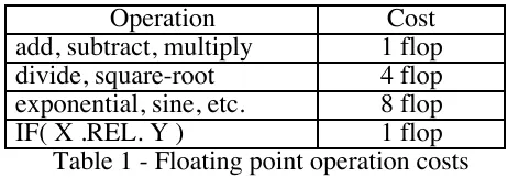
An example of principal operation characterisation in the performance studies of scientific applications are those based on floating point operations (or flops) [12, 16, 19]. The number of flops, that are to be credited for different types of floating point operations can be based on the scheme suggested by McMahon [25]. Using Table 1 one can use flops as the RUV for each node of the software execution graph. Then by using the flop rate (Mflop/s) of a specific system the execution time can be estimated.

Operation Cost

add, subtract, multiply 1 flop divide, square-root 4 flop exponential, sine, etc. 8 flop

IF( X .REL. Y ) 1 flop

Table 1 - Floating point operation costs

Principal operation characterisation conforms to an abstract based, macro classification methodology. It can be used at various stages of software development. The main advantages of this characterisation method is its high portability and the low effort required to obtain the principal operations. The main disadvantages of this method is its resulting low accuracy, and the limited applicability to applications that don't use the type of operations that have been selected, e.g. in non floating point intensive applications where flops has been selected as the principal operation.

3.3.3 High level language characterisation (HLLC)

Here the resource information is described through an analysis of the operations used in a high level language. An n-value vector is defined where each component represents the performance of a particular language operation. The components of the vector are a set of primitive operations that are found in a high level language, e.g.:

c=

(

)

where c is the operation cost vector, t_intadd, t_intsub, t_intdiv are the times required for an integer addition, subtraction, and division respectively, t_loop is the overhead for a loop operation, and t_if is the time overhead for an if statement and so on. The number of operations represented by this vector depends on the language, and the detail of analysis required.

The values of these parameters can be measured by a benchmarking procedure which isolates, and measures the performance of each operation. Each node of the software execution graph can be represented in terms of these primitive operations by analysing the source code of the program that corresponds to the graph node. A RUV is generated corresponding to the operation cost vector above that contains the frequency of each operation, e.g.:

f =

(

)

where f is the RUV, fintadd, fintsub, fintdiv are the frequencies of the integer addition,

The execution time, t_x, of each node of the software execution graph is given by the inner product of the operation cost vector and the RUV:

t_x =cT⋅f (4)

High level language characterisation has been used in many performance studies, e.g. [3, 10, 31, 34]. Languages that have been characterised in this way include FORTRAN [3, 31], and Pascal [34].

The generation of control flow graphs and automatic estimation of resource usage in terms of the high level language constructs was first described by Cohen [10]. A more pragmatic approach was followed in [3] where the performance of FORTRAN scientific programs is analysed using high level language characterisation for a range of systems from workstations, up to supercomputers each having a different operation cost vector. In [34] a micro time cost analysis methodology is presented for parallel computations. A sub-set of PASCAL was used as the target language and a tool (TCAS) described that allows the automatic generation of control flow graphs of the program and automatic estimation of RUVs. Finally in [31] an interpretative framework for application performance prediction is presented targeted mainly on heterogeneous high performance computing systems. A tool is presented that can estimate HPF FORTRAN programs automatically. As in the TCAS tool part of the interpretative performance tool includes the estimation of the RUVs in terms of HPF FORTRAN constructs.

Although these last two tools describe parallel system characterisations, the TCAS tool is limited to a shared memory system where no-contention in accessing memories is considered (an idealised system), and the HPF-FORTRAN was analysed through its implicit data-parallelism. Thus their applicability to general parallel systems is yet to be developed.

High level language characterisation is an attractive methodology because it allows the software characterisation to be performed in a system independent fashion. Since the software is characterised in terms of RUVs, the performance can be predicted for any system by using the system dependent operation cost vector. Another advantage of the method is that it only requires the source code of the program for estimating the resource usage without the need of a compiler for the system under investigation or the actual system to obtain measurements. The effort required in obtaining the frequency of operations is relatively small and can be performed automatically in many cases. However, the operation cost vector approach considers non-overlapping independent operations and does not lend itself readily to optimising compilers and to super-scalar processors (which allow multiple operations to take place simultaneously).

3.3.4 Intermediate code characterisation (IntCC)

Another characterisation approach similar to the high level language is intermediate code characterisation. Instead of analysing the high level language operations, intermediate code as output from a compiler is examined. Since the intermediate code is closer to the assembly language, more detailed hardware models can be used which include parameters such as cache misses, branch behaviour, main memory access frequency etc. This methodology has been used for sequential benchmark characterisation [11].

hardware system model. It conforms to the micro and software based classifications presented earlier.

3.3.5 Instruction code characterisation (ICC)

Instruction code analysis is based on the statistical examination of the assembly code that is produced as the final output from a compiler. The result of this procedure is the derivation of a frequency table of the instructions that are executed within each node of the software execution graph. From the instruction frequency table, a RUV can be derived that can be used as input to a detailed resource model.

Examples of such resource models are the number of clock cycles for task execution, main memory references, cache hit ratios etc. A number of instruction code characterisations have been detailed previously, e.g. [13, 18, 23, 33, 42].

Instruction code analysis does not require the execution of the code on the target system, but requires only the system compiler. Predictions are obtained by evaluating the resource model with the RUV derived from the instruction frequency tables and provides higher accuracy than the other characterisation techniques described here. The main disadvantages of this method is that it requires relatively high effort in obtaining the RUVs, although tools can be used to accelerate the procedure (e.g. [42]), and the portability of the results obtained is low. Portability only across systems which contain the same processor component is possible. The resource model is applicable across a number of systems, but the parameters contained within it are system specific, (e.g. cycle time, pipeline length).

Instruction code analysis is a system based and a micro type characterisation method. It requires the measurement of all the operations produced as output by the compiler, and thus is software and processor dependent. However, its advantages is that it has the scope in producing the most accurate predictions from all characterisation methods described.

3.3.6 Component Timing (CT)

The last characterisation method is to actually measure the time required to execute each node of the software execution graph on the target system. This can be performed when the source code and the system are both available. Component timing is most appropriate for performance tuning, capacity planning, and when studying the effects of data dependent parameters.

Monitoring tools are widely available that allow the measurement of the execution time of each node of the software execution graph. Some examples of monitoring tools that can be used for this purpose are IPS-2 [26], PABLO [35], and PEPS monitoring tool [24]. Because of the available tools it is easy to perform performance studies using component timing as resource information and will result with high accuracy. However, component timing can only be used in the last stage of the software development when the source code and system are both available. Another disadvantage is that the timing information cannot be used on other systems.

Component timing cannot be considered as micro or macro analysis, since it does not involve the measurement of any operations, but can be classified as a system based characterisation.

3.4 Summary of characterisation resource models

examples. The design based and principal operation characterisation methods provide a systematic approach to approximate resource usage information for software from an algorithm or from the software design. They do not require the existence of source code, compiler, or the system itself, but the resulting accuracy is low.

The high level language characterisation and intermediate code analysis provides two system independent methods to predict performance. The accuracy obtained is high and different degrees of effort is required to obtain the resource usage information.

Finally, instruction code analysis and component timing can be used for system dependent studies, where the source code, compiler, and system are available. The accuracy of the predictions is typically high. The effort required for the instruction code analysis is typically high but for the component timing is typically low.

Method Classifications Requirements Phase of Portability Accuracy Effort Code Compiler System Develop.

DBC Macro,

Abstract

Design ***† * ***

POC Macro,

Abstract

Algorithm Design

Code

*** * *

HLLC Micro,

Software Based

✓ Code *** ** **

IntCC Micro, Software Based

✓ Code ** *** ***

ICC Micro,

System Based

✓ ✓ Code * *** ***

CT Monitoring, System Based

✓ ✓ ✓ Code None *** *

† _{* low, ** medium, *** high}

Table 2 - Overview of resource usage characterisation methods

4. Example Application Kernels

For the analysis of the different characterisation techniques three application kernels are used. These kernels have been implemented on a Parsytec MIMD parallel system and have been characterised using the layered characterisation framework, described in Section 2. A number of different resource models have been analysed on each kernel. The kernel applications are described below in terms of their software execution graphs and parallelisation strategies. This is followed by a description of the communication model and resource models.

4.1 Kernel descriptions

The kernel applications have been selected to represent commonly used operations that occur within many application processing domains. They can be considered as separate operations which have being individually analysed. The kernel applications were selected from the results of a study of the processing operations that commonly occur across many application domains [29].

iteration count, a conditional branch has a probability value of each branch occurring, and a RUV is used for each of the processing stages.

N

N P_edge

!P_edge

edge

power

power

vinit

ivals

srf

result

Surface Estimation Numerical Integration

Kernel

vinit

N_merge

merge

tail

copy

N_tail

N_copy

Merge Function Parallel Sort

N_cols

N_rows

dtpr

Dot Product Matrix Multiplication

v

v

v

v

v

v v v v

v

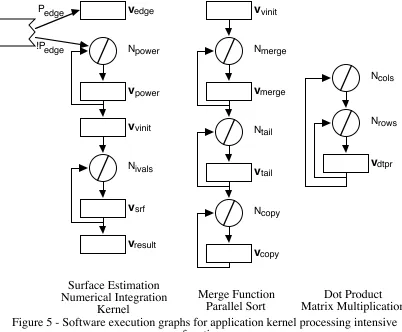
Figure 5 - Software execution graphs for application kernel processing intensive functions

It can be seen in Figure 5, that the surface estimation of the numerical integration kernel consists of 5 processing stages, 1 conditional branch, and 2 loops, whereas the dot product operation from the matrix multiplication kernel consists of a single processing stage embedded within a double nested loop.

The timing formula for the software execution graphs of each application kernel is shown in Table 3. This formula is simply the summation of the time taken for each of the processing stages, multiplied by their probability of occurring and by any loop iteration counts. Note that the function t() provides the execution time for the processing stages and represents the resource model.

Kernel Function Timing Formula

Integration Surface

Estimation tx =Pedge⋅t

( )

(

)

N_power⋅t

(

)

(

)

( )

(

)

(

)

Sorting Merge _t

x =t

( )

(

)

( )

N_copy⋅t

( )

Matrix

Multiplication

Dot Product

t_x =N_cols⋅N_rows⋅t

( )

The descriptions of the kernel applications above are within the application layer of the characterisation framework. The parallelisation aspects of these kernels are contained within the parallel template layer. This describes the computation and communication patterns that result from mapping the kernels onto the target parallel system. For the kernels used here the parallelisation methods used was a domain decomposition with different communication patterns for each kernel. In the case of the numerical integration this consisted of a multiphase structure [17], for the sorting kernel a butterfly style structure was used [4], and for the matrix multiplication a standard row-column broadcast structure was used [27]. A detailed description of the characterisation of the computation-communication patterns within the parallel template is out of the scope of this paper.

4.2 Hardware models for the Parsytec SuperCluster

The hardware system used in this study is a Parsytec SuperCluster with 128 T800 (25Mhz) transputer nodes. This system supports grid style topologies, uses a micro-kernel operating system (PARIX 1.2), and is hosted by a SUN workstation. In obtaining parameters for the hardware models and measurements for the kernel applications sole use of the systems was possible (i.e. there were no multi-user effects).

Four of the characterisation resource techniques previously described have been used to obtain performance predictions. The resource models cover a wide range of characterisation techniques ranging from design based, macro type analysis techniques to detailed, system based, micro type analysis techniques. The techniques considered are: principal operation characterisation (using flops as the principal operation), high level language characterisation (using C constructs), instruction level characterisation (using the T800 assembly code), and component timing of code segments (obtained from the PABLO monitoring tool).

The effects of the communication are considered separately from the computation components of the kernel applications. The underlying model used for the communication is the same across all characterisation techniques considered and thus it has been isolated to emphasise the differences in the resource models. The communication model encompasses part of the parallelism cost in contrast to the software execution graph that considers the serial parts of the application.

The model used for the Parsytec system is based upon a linear model parametrised in terms of inter-processor communication node distance, and message length (bytes). The model also contains values for communication start-up time, packet size, bandwidth etc. This model is based on the work done by Bomans [6] and has been extended for packet switching routing by Tron [40], and has not been modified here. The inaccuracies contained within the communication model are not of interest here and are separated out in the analysis that follows. The communication model is as follows:

t_com(l,d)=

α +d⋅

(

(

)

)

α +d⋅

(

)

 



⋅

(

)

   

(5)

where l is the message size, d distance between source and destination nodes, h is the size of the packet header, p the size of the packet, α is the time to prepare the message,

The parameters in this model are obtained through the regression of a set of measurements obtained for different values of l (from 100 to 20000 bytes) and d (from 1 to 10 node distances).

The resource models within the four characterisation techniques being considered are described in detail below. It is described which parameters within these resource models are required and whether they are obtained from measurements or system specifications. Note however, that there is no resource model when component timing is used.

4.2.1Principal operation characterisation

The principal operation characterisation used here, considers only floating point operations (flops). The RUV for each node of the software execution graph contains the type and frequencies of floating point operations. Using McMachon's weighting function, Table 1, a single value is calculated that represents the total number of flops. The resource model is this case consists of only the floating point rate of the processor, when combined with the flops value provides the predicted execution time, t_x:

t_x = Nflops

R_fpu (6)

where Nflops is the flops value for this node and Rfpu is the sustained Mflop/s rate of the processor. The Rfpu can be obtained from the specifications of the processor, or through benchmark measurements. In the case here, the value of this was taken to be 1.5 Mflop/s [20].

4.2.2 High level language characterisation

The resource model within the High Level Language Characterisation considered the construct that occur in the C programming language. A full set of these was not defined however a sub-set which encompassed all necessary constructs for the three application kernels was used.

In total 28 constructs were considered grouped into integer operations, floating point operations, double precision floating point operations, control flow statements, and local/global variable memory references. The time cost of each operation was measured using a benchmark routine taking the average of 1x104ּrepetitions while isolating the effects of loop overheads. The benchmarking process was based on a suggestion given by Barrera [3].

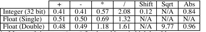
The time cost measured for most arithmetic operations is shown in Table 4 (NB not all operations are applicable to all types). Some of these measurements are not as expected (e.g. single floating point add/subtract compared with double floating point add/subtract). However, an understanding of these arithmetic costs is not required as long as an understood benchmarking process is used.

+ - * / Shift Sqrt Abs

Integer (32 bit) 0.41 0.41 0.57 2.08 0.12 N/A 0.84 Float (Single) 0.51 0.50 0.69 1.32 N/A N/A N/A Float (Double) 0.48 0.49 1.18 1.61 N/A 9.77 0.96

frequency of each operation. The execution time txfor each component of the software execution graph is calculated as in Equation 4.

4.2.3 Instruction level characterisation

The hardware model of the Instruction Level Characterisation is more complex than those in the other characterisation techniques analysed here. The model includes parameters concerned with instruction cycle counts, memory references, and overlapped operation between the transputer FPU and ALU. The model used here is based on that described in [43]:

t_x =

(

)

where nex is the total number of clock cycles for instruction execution, nin_mem is the number of internal memory references, nex_mem is the number of external memory references, ninst is the total number of instructions, nfpu_ovr is the number of cycles in which FPU and ALU are overlapped, tcyc is the processor cycle time, and e is an off-chip memory cost factor. For the Parsytec SuperCluster the value of e was taken to be 5 cycles and tcyc was 40ns.

The RUV for this model consists of the five parameters (Equation 7). They are obtained by the analysis of the assembly code output of the ACE C compiler. The value of nex is taken to be the sum of the frequency of each instruction multiplied by the cycle count for it. The parameters nin_mem and nex_mem are calculated from the number of memory references (and their addresses) in the operands of load and store instructions. The parameter ninst is taken to be the number of instructions executed and nfpu_ovr is calculated by the examination of the sequence of instructions performed. These parameters are obtained for each node of the software execution graph and the execution time, tx, is then calculated using the above hardware instruction level model.

5. Results

Presented here are prediction results and measurements for the three application kernels described earlier. For each, results are given for the characterisation techniques described in Section 4. The results were obtained from the implementation of the characterisation models within the Mathematica programming environment. This has also been used in previous characterisation and modelling studies [30, 32].

5.1 Comparison of measurements and characterisation predictions

The measurements and predictions have been obtained for the Parsytec SuperCluster. To measure elapsed time, a short assembly code routine was used that takes 6.5µsec to execute. For each of the application kernels (integration, sorting, and matrix multiplication) results are given for the four characterisation techniques, principal operation (flops), high level language (C language constructs), instruction level (transputer assembly), and component timing. These four methods are compared with the elapsed time measured for the complete kernel.

Node _CT† _ICC‡ _HLLC* _POC**

Surface Estimation - Integration

t_edge 37.0 37.1 29.6 12.0

t_power 3.1 3.6 2.1 0.0

t_vinit 8.8 10.4 7.0 5.4

t_srf 23.0 22.9 19.4 11.5

t_result 7.0 7.9 6.0 6.2

Merge - Sort

t_vinit 1.5 1.2 0.5 0.0

t_merge 12.1 10.8 9.2 0.8

t_tail 6.0 8 3.9 0.0

t_copy 8.9 9.2 5.6 0.0

Dot Product - Matrix Multiplication

t_dtpr 6.5 6.4 6.9 1.5

† _{Component Timing,} ‡ _{Instruction Code Characterisation,} * _{High Level Language Characterisation,} **ּ_{Principal Operation Characterisation}

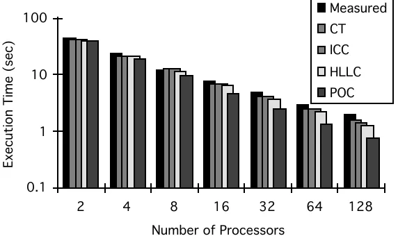
Table 6 - Software execution graph node predicted execution times (µsec) The measured and predicted total execution times are shown in Figures 6, 7, 8. These are for a range of processor numbers but on a fix sized data set. The data size for the sorting kernel was 128K floating point data elements, the matrix multiplication kernels for matrices of size 256x256, and in the integration kernel the integration interval was 0 to 100 of a fifth order polynomial with a final allowable precision of 1x10-10_.

Number of Processors

Execution Time (sec)

0.1 1 10

2 4 8 16 32 64 128

Measured CT ICC HLLC POC

Figure 6 - Measured and predicted times for the integration application kernel

Number of Processors

Execution Time (sec)

0.1 1 10 100

2 4 8 16 32 64 128

Measured CT ICC HLLC POC

Number of Processors

Execution Time (sec)

0.1 1 10 100

2 4 8 16 32 64 128

Measured CT ICC HLLC POC

Figure 8 - Measured and predicted times for matrix multiplication application kernel

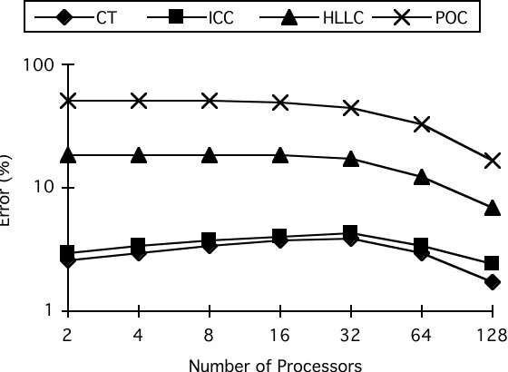
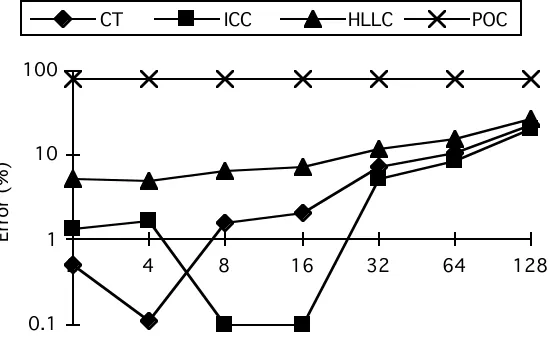
The difference between each of the predictions and the measurements has been calculated and shown in Figures 9, 10, 11 for each of the kernels. This can be considered as the overall error in each of the characterisation techniques. This error includes the parallel template, communication, software execution graph approximations, and the effect of the different resource usage techniques. These effects are separated out and discussed in the next section.

Number of Processors

Error (%)

1 10 100

2 4 8 16 32 64 128

CT ICC HLLC POC

Figure 9 - The error (%) between measured and predicted total execution times for the integration kernel

5.2 Discussion of results

• Resource Models: Errors due to the assumptions within the different techniques for characterising the resources.

• Software Execution Graph Approximations: Errors due to software control flow approximations.

• Parallel Template: Approximations made in the modelling of the parallelisation strategies.

• Communication Model: Inaccuracies in the communication model (e.g. network contention, synchronisation overheads).

• Other Effects: These include errors due to other characterisation and modelling techniques embedded into the framework, e.g. regression models that represent the performance of software and hardware components that cannot be otherwise characterised.

Number of Processor

Error (%)

0.1 1 10 100

2 4 8 16 32 64 128

CT ICC HLLC POC

Figure 10 - The error (%) between measured and predicted total execution times for the sorting kernel

Number of Processor

Error (%)

0.1 1 10 100

2 4 8 16 32 64 128

CT ICC HLLC POC

Within the analysis here only the errors due to the different resource usage models are of interest. These can be separated out from the overall errors presented in section 4 as follows.

The errors associated with the last four categories are the same for the characterisation techniques used. However, the first category depends upon the resource model in the characterisation technique (in the case of component timing this is zero). Thus by subtracting the resulting errors in the component timing from the errors in the predicted times of the other characterisation techniques, the errors only due to the resource models can be separated. The errors due only to the resource model within the characterisation techniques are shown in Table 6 for the three kernels.

Integration Sorting Matrix Multiplication

Processors _ICC† _HLLC‡ _POC* ICC HLLC POC ICC HLLC POC

2 0.3% 15.5% 48.6% 0.4% 1.4% 4.8% 0.8% 4.8% 80.5%

4 0.4% 15.4% 48.4% 0.5% 3.7% 12.4% 1.6% 4.9% 79.9%

8 0.3% 15.2% 47.7% 0.6% 5.3% 21.4% 1.5% 4.9% 79.2%

16 0.3% 14.7% 46.1% 0.3% 9.0% 29.4% 2.0% 5.1% 78.0%

32 0.4% 13.2% 41.1% 0.1% 12.3% 40.0% 1.8% 4.8% 72.8%

64 0.5% 9.5% 29.8% 0.1% 12.5% 40.6% 1.9% 5.2% 69.0%

128 0.7% 5.1% 15.1% 0.7% 5.1% 15.1% 1.6% 4.3% 57.2%

† _{Instruction Code Characterisation,} ‡ _{High Level Language Characterisation,} * _{Principal Operation}

Characterisation

Table 6 - Error in Predictions due to Resource Models

It can be seen from this table that the error increases between the instruction level characterisation to the high level characterisation and similarly between the high level characterisation to the principal operation characterisation. This is as expected due to the increase of complexity in the resource models and RUVs between the more abstract methods and the detailed instruction level characterisation. These effects where discussed in Section 3 but can now be quantified.

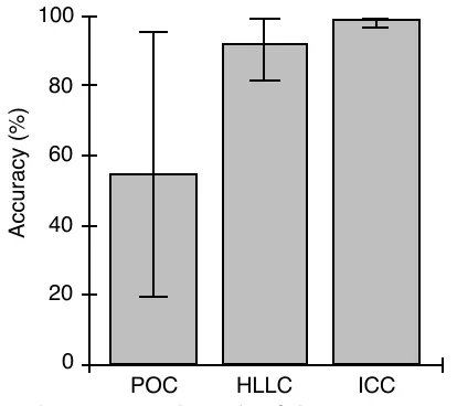
The variation in Table 6 for different processor numbers is due to different weightings that are placed on the components of each software execution graph such as the looping iterations, and the conditional branches which are parametrised in terms of the number of processors. In the case of the multiplication kernel it can be seen that errors in the principal operation characterisation are large. This is due to the core computation (the dot product calculation) consisting of a single multiply - accumulate operation nested within a double loop. The principal operation characterisation does not considers the looping overheads (consisting of only integer operations). The accuracy bounds for each of the resource models in the characterisation techniques are shown in Figure 12. It is clearly shown here the different bounds in accuracy that each of these methods produced for the kernels analysed. The values of the mean error (%), standard deviation, minimum and maximum errors, and the 90% confidence interval of the mean are tabulated in Table 7.

Method Mean

Standard Deviation

Error Bounds (Min, Max)

90% Confidence Interval of Mean

ICC† 0.80 0.64 (0.10, 2.00) (0.57, 1.030)

HLLC‡ 8.19 4.65 (1.40, 15.50) (6.52, 9.85)

POC* 45.58 24.31 (4.80, 80.50) (36.86, 54.3)

† _{Instruction Code Characterisation,} ‡ _{High Level Language Characterisation,} * _{Principal Operation}

Characterisation

20 40 60 80 100

0

Accuracy (%)

POC HLLC ICC

Figure 12 - Accuracy bounds of the resource models

6. Summary

In this paper, characterisation techniques have been examined and classified into a number of categories depending upon the complexity of the resource models. Commonly, each characterisation technique involves a description of the underlying hardware which is combined with resource usage information to enable predictions of the execution time to be made. The emphasis on the analysis of the resource models has been to quantify their effects when applied to parallel systems. For this purpose this analysis has been performed within a characterisation framework which also encompasses aspects of parallel systems. The effects that the framework have on the accuracy of resulting predictions is separated so that the full effect of the resource models can be quantified.

The characterisation techniques in common use range from abstract levels involving little resource information through to detailed low level information. These were: abstract characterisation, principal operation characterisation, high level language characterisation, intermediate language characterisation, instruction code characterisation, and component timing characterisation. The advantages and disadvantages of each technique was discussed.

Representative characterisation techniques were used on three application kernels (integration, sorting, matrix multiplication) to demonstrate and compare the accuracy of each method. The characterisation techniques used were principal operation (flop), high level language (C constructs), instruction level (transputer assembly), and component timing analysis (obtained from monitoring information).

The results obtained for the different resource models have illustrated that the more detailed the resource model used is then the more accurate the resulting predictions are. For the software kernels and the hardware considered the error bounds due only to resource usage information in each of the characterisation techniques ranged between 0.1-2.0%, 1.4-15.5%, 4.8-80.5% for the instruction level characterisation, high level language characterisation, and principal operation characterisation respectively.

Acknowledgements

This work is funded in part by the ESPRIT project 6942 (PEPS) - Performance Evaluation of Parallel Systems. The authors wish to thank the members of the Parallel Systems Group for their support and discussions on this work.

References

[1] R.A. Ammar, J. Wang, and H.A. Sholl, Graphic modelling technique for software execution time estimation, Information and Software Technology33 (2) (1991) 151-156.

[2] R.A. Ammar, Experimental-analytic approach to derive software performance, Information and Software Technology34 (4) (1992) 229-238.

[3] R.H. Saavedra-Barrera, A.J. Smith, and E. Miya, Machine characterisation based on an abstract high-level language machine, IEEE Trans. on Computers38 (12) (1989) 1659-1679.

[4] K. Batcher, Sorting networks and their applications, in: Proc. AFIPS Spring Joint Summer Computer Conf. (1968) 307-314.

[5] B. Beizer, Software performance, in: C.R. Vick and C.V. Ramamoorthy, eds., Handbook of Software Engineering (New York, 1984) 413-436.

[6] I. Bomans and D. Roose, Benchmarking the iPSC/2 hypercube multicomputer, Concurrency: Practice and Experience1 (1) (1989) 3-18.

[7] T.L. Booth, Use of computation structure models to measure computation performance, in: Proc. Conference on Simulation, Measurement and Modeling of Computer Systems, USA (1979). [8] M. Calzarossa and G. Serazzi, Workload characterisation: a survey, Proceeding of the IEEE81 (8)

(1993) 1136-1150.

[9] P.P. Chang, S.A. Mahlke, W.Y. Warter, W.W. Hwu, IMPACTּ-ּAn architectural framework for multiple-instruction-issue processors, in: Proc of the 18th Annual International Symposium on Computer Architecture, Toronto, Canada (1991) 266-275.

[10] J. Cohen, Computer-assisted microanalysis of programs, Communications of the ACM 25 (10) (1982) 724-733.

[11] T.M. Conte, W.W. Hwu, Benchmark characterisation, IEEE Computer24 (1) (1991) 48-56. [12] J.J. Dongarra, Performance of various computers using standard linear equations software,

Technical Report CS-89-85, University of Tennessee, USA, 1992.

[13] J.S. Emer and D.W. Clark, A characterization of processor performance in the VAX-11/780, in:

Proc. of the 11th Annual Internation Symosium on Computer Architecture (1984) 301-310. [14] D. Ferrari, G. Serazzi, and A. Zeigner, Measurement and Tuning of Computer Systems

(Prentice-Hall, New Jersey, 1983).

[15] R.F. Freund and H.J. Siegel, Heterogeneous processing, IEEE Computer26 (6) (1993) 13-17. [16] V. Getov, 1-Dimensional parallel FFT benchmark on SUPRENUM, in: D. Etiemble and J.C. Syre,

eds., PARLE'92, Lecture Notes in Computer Science, Vol. 605 (Springer-Verlag, 1992) 163-174. [17] E.F. Gehringer, D.P. Siewiorek, and Z. Segall, Parallel Processing: The CM* Experience (Digital

Press, 1989).

[18] J.L. Hennessy and D.A. Patterson, Computer Architecture: A Quantitative Approach (Morgan Kaufmann Publishers, 1990).

[19] R.W. Hockney, Performance parameters and benchmarking of supercomputers, in: J.J. Dongarra and W. Gentzsch, eds., Computer Benchmarks (Elsevier Science Publishers, Holland, 1993) 41-63. [20] M. Homewood, D. May, D. Shepherd, and R. Shepherd, The IMS T800 transputer, IEEE Micro 7

(5) (1987) 10-26.

[21] R. Jain, The Art of Computer Systems Performance Analysis (John Wiley & Son, New York, 1991).

[22] T. Jennings and C.U. Smith, GQUE: Using workstation power for software design assessment, Technical Report, L&S Computer Technology Inc., USA, 1987.

(Addison-[24] A. Marconi, M.R. Nazzarelli, and S. Sabina, Design issues in performance monitoring of parallel systems: the PEPS approach, in: Proc. of Performance Evaluation of Parallel Systems, Coventry, U.K. (1993) 59-66.

[25] F.H. McMahon, The Livermore Fortran Kernels test of the numerical performance range, in: J.L. Martin, eds., Performance Evaluation of Supercomputers (North Holland, Amsterdam, 1988) 143-186.

[26] B.P. Miller, M. Clark, J. Hollingsworth, S. Kierstead, S.S. Lim, and T. Torewski, IPS-2: The second generation of a parallel program measurement system, IEEE Trans. on Parallel and Distributed Systems1 (2) (1990) 206-217.

[27] J.J. Modi, Parallel Algorithms and Matrix Computation (Clarendon Press, Oxford, 1988).

[28] G.R. Nudd, E. Papaefstathiou, Y. Papay, et. al., A layered approach to the characterisation of parallel systems for performance prediction, in: Proc. of Performance Evaluation of Parallel Systems, Coventry, U.K. (1993) 26-34.

[29] G.R. Nudd, T.J. Atherton, D.J. Kerbyson, et.al., Characterisation of processing needs, Document D5.1, Esprit III Project 6942 (PEPS), University of Warwick, U.K., 1993.

[30] E. Papaefstathiou, D.J. Kerbyson, G.R. Nudd, A layered approach to parallel software performance prediction: A case study, in: J.C. Zuidervaart and L. Dekker, eds., Proc. of the 1994 EUROSIM Conf. on Massively Parallel Processing (Elsevier, 1994).

[31] M. Parashar, S. Hariri, T. Haupt, and G.C. Fox, An interpretive framework for application performance prediction, Technical Report SCCS-479, Syracuse University, USA, 1993.

[32] M.N. Patel, Structuring analytical performance models using Mathematica, in: R. Pooley and J. Hillston, eds., Proc. of the 6th International Conf. on Modelling Techniques and Tools for Computer Performance Evaluation (1992) 273-286.

[33] B.L. Peuto and L.J. Shustek, An instruction timing model of CPU performance, in: Proc. of the 4th Annual Symposium on Computer Architecture (1977) 165-178.

[34] B. Qin, H.A. Sholl, R.A. Ammar, Micro time cost analysis of parallel computations, IEEE Trans. on Computers40 (5) (1991) 613-626.

[35] D.A. Reed, R.Aydt, T.M. Madhyastha, R.J. Nose, K.A. Shields, and B.W. Schwartz, An overview of the Pablo performance analysis environment, Technical Report, University of Illinois, U.S.A., 1992.

[36] H. Sholl and T. Booth, Software performance modeling using computation structures, IEEE Trans. Software Eng.SE-1 (4) (1975).

[37] C.U. Smith, The prediction and evaluation of the performance of software from extended design specifications, Ph.D. Thesis, University of Texas at Austin, USA, 1980.

[38] C.U. Smith, Performance Engineering of Software Systems (Addison-Wesley Publishing Co., Inc., 1990).

[39] R.M. Stallman, Using and porting Gnu CC, Technical Report, Free Software Foundation, Cambridge, Mass., USA, 1989.

[40] C. Tron and B. Plateau, Modelling communication in parallel machines within the ALPES project, in: Performance Evaluation of Parallel Systems, Coventry, U.K. (1993) 110-117.

[41] M. Veran and D. Potier, QNAP2: A portable environment for queueing systems modelling, in:

Proc. of International Conference on Modelling Techniques and Tools for Performance Analysis, Paris, France (1984).

[42] M.J. Zemerly, E. Papaefstathiou, T.J. Atherton, D.J. Kerbyson, and G.R. Nudd, Characterising computational kernels, in: Proc of the Performance Evaluation of Parallel Systems Conference, Coventry, U.K. (1993) 231-237.