An efficient sparse regularity concept

Original citation:

Coja-Oghlan, Amin, Cooper, Colin and Frieze, Alan. (2010) An efficient sparse regularity

concept. SIAM Journal on Discrete Mathematics, Vol.23 (No.4). pp. 2000-2034. ISSN

0895-4801

Permanent WRAP url:

http://wrap.warwick.ac.uk/5351

Copyright and reuse:

The Warwick Research Archive Portal (WRAP) makes this work by researchers of the

University of Warwick available open access under the following conditions. Copyright ©

and all moral rights to the version of the paper presented here belong to the individual

author(s) and/or other copyright owners. To the extent reasonable and practicable the

material made available in WRAP has been checked for eligibility before being made

available.

Copies of full items can be used for personal research or study, educational, or

not-for-profit purposes without prior permission or charge. Provided that the authors, title and

full bibliographic details are credited, a hyperlink and/or URL is given for the original

metadata page and the content is not changed in any way.

Copyright statement:

“First Published in SIAM Journal on Discrete Mathematics in Volume 23 and Number 4,

published by the Society of Industrial and Applied Mathematics (SIAM)

http://dx.doi.org/10.1137/080730160”

“Copyright © by SIAM. Unauthorized reproduction of this article is prohibited.”

A note on versions:

The version presented in WRAP is the published version or, version of record, and may

be cited as it appears here.

AN EFFICIENT SPARSE REGULARITY CONCEPT∗

AMIN COJA-OGHLAN†, COLIN COOPER‡, ANDALAN FRIEZE§

Abstract. LetAbe a 0/1 matrix of sizem×n, and letpbe the density ofA(i.e., the number of ones divided bym·n). We show thatAcan be approximated in the cut norm withinε·mnp by a sum of cut matrices (of rank 1), where the number of summands is independent of the size

m·nofA, provided that Asatisfies a certain boundedness condition. This decomposition can be computed in polynomial time. This result extends the work of Frieze and Kannan [Combinatorica, 19 (1999), pp. 175–220] tosparsematrices. As an application, we obtain efficient 1−εapproximation algorithms for “bounded” instances of MAX CSP problems.

Key words. approximation algorithms, regularity lemma, matrix decomposition, cut norm, random discrete structures

AMS subject classifications.05C85, 05C65

DOI.10.1137/080730160

1. Introduction and results. For many fundamental optimization problems there are known NP-hardness of approximation results, showing that not only is it NP-hard to compute the optimum exactly but even to approximate the optimum within a factor bounded away from 1. For instance, in the MAX_k-SAT problem it is NP-hard to achieve an approximation ratio better than 1−2−k [21]. Furthermore, it is NP-hard to approximate MAX CUT within better than 16_/17≈0_.94118 [21, 26] (which can be tightened to≈0_.87856 under a stronger hypothesis [22]).

Frieze and Kannan [17] showed that the situation is much better fordense prob-lem instances. For example, if _G = (_{V, E}) is a graph on _n vertices of density p = 2_n−2|_E|, then its MAX CUT can be approximated within a factor of 1−_ε in time poly(exp((_εp)−2)·_n). Hence, if_{p > δ} for some fixed number_{δ >}0, then this algorithm has a polynomial running time. Similarly, if_F is a_k-SAT formula with at least_δ2kn_kclauses (i.e., at least a constant fraction of all possible clauses is present), then the maximum number of simultaneously satisfiable clauses can be approximated within 1−_εin polynomial time for any fixed_{ε >}0.

The key ingredient in [17] is an algorithm for approximating a dense matrix A by a sum of a bounded number of “cut matrices.” Applied to the adjacency matrix of a graph, this yields the aforementioned algorithm for MAX CUT. Moreover, an extension of this matrix algorithm to_k-dimensional tensors yields the approximation algorithms for dense instances of MAX CSP problems. To explain the matrix de-composition, let us consider a 0_/1 matrix A of size _m×_n, and let 0 ≤ _p ≤ 1 be thedensity ofA, i.e., the number of ones in Adivided by _m·_n. Acut matrix is a matrix D such that there are sets_S ⊂[_m], _T ⊂ [_n] and a number_d such that the

∗_{Received by the editors July 14, 2008; accepted for publication (in revised form) October 12,}

2009; published electronically January 6, 2010. An extended abstract of this paper appeared in

Proceedings of the Twentieth ACM-SIAM Symposium on Discrete Algorithms, 2009, pp. 207–216. http://www.siam.org/journals/sidma/23-4/73016.html

†_{University of Edinburgh, School of Informatics, 10 Crichton Street, Edinburgh EH8 9AB, UK}

([email protected]). This author’s research was supported by grant DFG CO 646 and was done while visiting Carnegie Mellon.

‡_{Department of Computer Science, King’s College, University of London, London WC2R 2LS, UK}

([email protected]). This author’s research was supported by Royal Society grant 2006/R2-IJP.

§_{Department of Mathematical Sciences, Carnegie Mellon University, Pittsburgh, PA 15213 (alan@}

random.math.cmu.edu). This author’s research was supported in part by NSF grant CCF0502793.

entryD_ij is equal to_dif (_{i, j})∈_S×_T and 0 otherwise. We denote such a matrix by D= CUT(_{d, S, T}) and observe that cut matrices have rank one. Thecut norm of a m×nmatrixM= (M_ij)_{i∈[m],j∈[n]} is

M₂= max

S⊂[m],T⊂[n]|M(S, T)|, where

M(_{S, T}) = (s,t)∈S×T

M_st.

Frieze and Kannan proved that for any A and any _{ε >} 0 there exist cut matrices D_{1, . . . ,}D_s such that

A−(D₁+· · ·+D_s)_{2< ε}·_mn,

where_s≤_cε−2 for a constant_{c >}0. Indeed, such a decomposition can be computed in time _ε−2·poly(_mn) (or even in “constant” expected time _O(_ε−2·polylog(1_/ε)) by sampling). Hence, if _p ≥ _δ for some fixed _{δ >} 0, i.e., if A is a dense matrix, then setting_ε =_εpwe can use this algorithm to find a decomposition ofA within εA₂ = _ε·_mnp efficiently by a sum of at most _cε−2 = _c(_εp)−2 ≤ _c(_εδ)−2 cut matrices. The crucial point here is that the number of cut matrices is bounded independently of the size_m·_nofA.

The goal of the present paper is to extend this result to sparse matrices, where the density_pofAis no longer bounded below by a fixed number. Thus, in asymptotic terms, we are interested in _p=_o(1) as _{m, n}→ ∞. Clearly, in this case the bound c(_εp)−2on the number of cut matrices in the decomposition guaranteed by [17] is no longer “constant” but grows with the size _m·_nof A. Of course, we cannot expect to obtain the same results as in the dense case for arbitrary sparse matrices. This is because in light of the aforementioned hardness results this would imply P = NP. Hence, our main result is that even in the sparse case a 0_/1 matrix A (or, more generally, a_k-dimensional tensor) can be approximated in the cut norm by a sum of cut matrices with a number of summands independent of_m,_n, and_p,provided that

Asatisfies a certain boundedness condition. This condition basically requires thatA does not feature relatively large, extraordinarily dense spots. In addition, we shall use these decomposition results to obtain (1−_ε)-approximation algorithms for instances of MAX CSP problems that have a suitable boundedness property. As we shall see, in a sense these results mediate between the “average” and the worst-case analysis of algorithms.

Outline. In this section we state our results and discuss related work. Section 2 contains a few preliminaries, and in section 3 we present the algorithms and their analyses for decomposing matrices and graphs. Further, in section 4 we deal with k-dimensional tensors. Then, in section 5 we apply the tensor algorithm to approxi-mate MAX CSP problems. Finally, section 6 contains a few examples, which link our results to the “average case” analysis of algorithms.

1.1. Approximating 0/1 matrices. LetAbe a 0_/1 matrix of size_m×_nand density_p. Given_{C, γ >}0, we say thatAis (_{C, γ})-bounded if for any two sets_S⊂[_m] and_T ⊂[_n] of sizes|_S| ≥_γm,|_T| ≥_γnwe have

(1) A(_{S, T}) =

(s,t)∈S×T

In other words, for any two sufficiently large sets_{S, T} the numberA(_{S, T}) of ones in the square_S×_T must not exceed the number|_S| · |_T| ·_pthat we would expect if_{S, T} wererandom sets by more than a factor of_C.

Theorem 1. _{There exist an algorithm ApxMatrix, absolute constants ζ} ≥ _1, 0_{< ζ}≤1, and a polynomialΠsuch that the following holds. Suppose that0_{< ε <} 1₂ and_{C >}1. Let

(2) _κ=ζC

2

ε2 and γ=γ(ε, C) = ζε 210κ_C.

If A is a (_{C, γ})-bounded 0_/1 matrix, then in time _κ·Π(_m·_n), ApxMatrix(A_{, C, ε}) outputs cut matrices D_{1, . . . ,}D_s such that _s ≤ _κ and A−(D₁+· · ·+D_s)₂ ≤ εA_2.

We emphasize that the upper bound _κon the number of cut matrices depends only on_C and _εbut not on the size ofA or the density_p. Also observe that, as A is a 0_/1 matrix,A₂=_mnpis just the “number of ones” inA.

Given the 0_/1 matrixAand partitionsS of [_m] andT of [_n], we define a matrix A_S×T as follows. If_s∈_S∈ Sand_t∈_T ∈ T, then the corresponding entry (A_S×T)_s,t equals|_S|−1|_T|−1A(_{S, T}). Hence, on each square_S×_Tthe matrixA_S×T is constant, and the value it takes is just the average ofAover that square.

Corollary 2. There exist an algorithm _PartMatrix and a polynomial Π that

satisfy the following. Suppose that _{ε, C >} 0, let _{κ, γ} be as in (2), and assume that A is a (_{C, γ})-bounded 0_/1 matrix of size _m×_n. Then in time 2κ·Π(_m·_n) PartMatrix(A_{, C, ε}) computes partitions S of [_m] and T of [_n] such that

A−A_S×T2 ≤ 2_εA_2. The number of classes in each partition S, T is at most2κ.

1.2. Weak regular partitions of graphs. Let _G = (_{V, E}) be a graph on _n vertices, and let 0≤_p≤1 be such that|_E|=_n2_p/2. We refer to_pas thedensityof_G. Moreover, we assume that _V = [_n]. Let A =A(_G) be the adjacency matrix of _G. We say that_Gis (_{C, γ})-bounded ifAhas this property. Thus, if_Gis (_{C, γ})-bounded, then for any two sets_{S, T} ⊂_V of size at least_γn we have_eG(_{S, T})≤_Cγ|_S×_T|_p, where_eG(_{S, T}) is the number of_S–_T-edges in_G.

We call a partition V of _V a weak _ε-regular partition of _Gif A−A_V×V2 ≤ εA₂= 2_ε|_E|. Hence, if, for instance,_{S, T} ⊂_V are disjoint sets of vertices, then the number A(_{S, T}) of_S–_T-edges is within 2_ε|_E|of A_V×V(_{S, T}). As we shall see below, this definition is related to the notion of regular partitions introduced by Szemer´edi. Corollary 3. _{There exist an algorithmWeakPartitionand a polynomialΠthat}

satisfy the following. Suppose that_{C >}1and0_{< ε <} 1₂, let_{κ, γ >}0be as in(2), and let_G= (_{V, E})be a(_{C, γ})-bounded graph on_nvertices. Then_{WeakPartition}(_{G, C, ε}) computes a weak 4_ε-regular partition of_G in time 22κ·Π(_n). This partition has at most22κ classes.

1.3. Approximatingk-dimensional 0/1 tensors. A_k-dimensional tensor is a mapM: _R1×_R2×· · ·×_Rk→R, where_{R1, . . . , Rk} are finite index sets. Moreover, extending the matrix case to_kdimensions, we say thatC: _R1×_R2× · · · ×_Rk →R is acut tensor if there exist sets_Si⊆_Ri for_i= 1_,2_{, . . . , k}and a real number_dsuch that

C(_{i1, i2, . . . , ik}) =

In this case we write C= CUT(_{d, S1, . . . , Sk}). Further, we define the cut norm of a tensor as

M₂= max

Si⊆Ri|M(S1, S2, . . . , Sk)|, where

M(_{S1, . . . , Sk}) = (s1,...,sk)∈S1×···×Sk

M(_{s1, . . . , sk})_.

Let A: _R1×_R2× · · · ×_Rk → {0_,1} be a 0_/1 tensor. Set _k1 =_k/2. Then letting R = _R1×_R2× · · · ×_Rk1 and C = _Rk1+1×_Rk1+2× · · · ×_Rk, we define a (2-dimensional) matrixB=B(A) :R × C → {0_,1}by

(3) B((_{i1, i2, . . . , ik1})_,(_{ik1+1, ik1+2, . . . , ik})) =A(_{i1, i2, . . . , ik})_.

We say thatAis (_{C, γ})-bounded ifB(A) has this property.

Theorem 4. There exist an algorithm _ApxTensor, a polynomial Π, and a

con-stant Γ _> 1 such that the following is true. Suppose that _{C >} 1 and 0 _{< ε <} 1₂. Let

γ= exp(−Γ(_C/ε)2)_.

IfA: _R1×_R2×· · ·×_Rk→ {0_,1}is a(_{C, γ})-bounded0_/1tensor,ApxTensor(A_{, C, ε}) outputs cut tensors

D_i =CUT(_{di, Si}1_{, . . . , Si}k) (_Si1⊂_{R1, . . . , S}k_i ⊂_Rk)

for _i= 1_{, . . . , s}with_s≤(Γ_C/ε)2(k−1)such that

A−(D₁+· · ·+D_s)₂≤_εA_2.

Moreover, s_i=1d2_i ≤ (_Cp)2Γ2k_. The running time is (expΓ(_C/ε)2+ (Γ_C/ε)3k)· Π(|_R1× · · · ×_Rk|).

IfR_{1, . . . ,}R_k are partitions of_{R1, . . . , Rk}, then we define a tensor A_{R1×···×Rk} : R1× · · · ×Rk →[0_,1] as follows: if_ti∈_ρi∈ R_i for_i= 1_{, . . . , k}, then we set

A_{R1×···×Rk}(_{t1, . . . , tk}) = A(ρ1, . . . , ρ_k k)

i=1|ρi| =

(v1,...,vk)∈ρ1×···×ρkA(v1, . . . , vk)

_k

i=1|ρi|

.

In other words, on every rectangle_ρ1× · · · ×_ρk made up of partition classes_ρi∈ R_i the entry ofA_{R1×···×Rk} is the average ofAover that rectangle.

Corollary 5. _{There exist an algorithm PartTensor, a polynomial Π, and a}

constant Γ˜ _>0 such that the following is true. Suppose that _{C >}0 and 0 _{< ε <} 1₂. Let _γ= exp(−Γ(˜ _C/ε)2)_. IfA: _R1×_R2× · · · ×_Rk → {0_,1} is a(_{C, γ})-bounded0_/1 tensor, thenPartTensor(A_{, C, ε})computes partitions R_{1, . . . ,}R_k of _{R1, . . . , Rk} such that

A−A_{R1×···×Rk2< ε}A_2.

Each of the partitionsR_i consists of at mostexp((˜Γ_C/ε)2(k−1))classes. The running time is bounded by

1.4. An approximation algorithm for bounded MAX CSPs. Let _V =

{x1, . . . , xn}be a set ofnBoolean variables. A(binary)k-constraint overV is a map

φ:{0_,1}Vφ → {0_,1} that is not identically zero, where_Vφ ⊂_V is a set of size _k. For an assignment _σ∈ {0_,1}V we let _φ(_σ) =_φ((_σ(_x))_x∈Vφ). Further, a _k-CSP instance over_V is a setF of_k-constraints over _V, and we define

OPT(F) = max

σ∈{0,1}V

φ∈F

φ(_σ)_.

We let Ψ = Ψ_k be the set of all 22k −1 nonzero maps {0_,1}k → {0_,1}. Let ψ∈Ψ, and let_φ:{0_,1}Vφ → {0_,1}be a_k-constraint, where_Vφ={_{xi1, . . . , xik}}with 1 ≤_{i1 <}· · · _{< ik} ≤_n. Then we say that _φ is of type _ψ if for any_σ :_Vφ → {0_,1} we have _ψ(_σ(_xi1)_{, . . . , σ}(_xik)) = _φ(_σ). With this notion we can represent a _k-CSP instance F by a family (Aψ_F)_ψ∈Ψ of 22k −1 _k-tensors as follows. For any tuple (_{i1, . . . , ik})∈[_n]k we let

Aψ_F(_{i1, . . . , ik}) =

1 if there is_φ∈ F of type_ψ with_Vφ ={_{xi1, . . . , xik}},

0 otherwise.

Further, we say thatFis (_{C, γ})-boundedif all tensorsAψ_F are (_{C, γ})-bounded (_ψ∈Ψ). Theorem 6. There exist an algorithm_ApxCSP, a constant Γ>0, and a

polyno-mialΠ such that for any_{k, C >}1,0_{< ε < 2}1 there is a number_n0=_n0(_{C, ε, k})such that the following is true. Let

γ= exp(−Γ22k+2k+2(_C/ε)2)_.

If F is a (_{C, γ})-bounded _k-CSP instance over _V = {_{x1, . . . , xn}} for some _n ≥ _n0, thenApxCSP(F_{, C, ε})outputs an assignment_σ:_V → {0_,1} such that

φ∈F

φ(_σ)≥(1−_ε)OPT(F)_.

The running time is at mostΠ[exp(_k2k22k(Γ_C/ε)2kln(_C/ε))_nk].

1.5. Related work.

1.5.1. Approximating dense matrices and tensors. As mentioned earlier, Frieze and Kannan [17] dealt withdense matrices and tensors. More precisely, they showed that given a tensor A : _R1 × · · · ×_Rk → [0_,1] and _{ε >} 0 one can com-pute cut tensorsD_{1, . . . ,}D_s such thatA−s_i=1D_{i2 < ε}|_R1× · · · ×_Rk| in time O(_ε2(1−k)polylog(1_/ε)) with_s≤_O(_ε)2(1−k) as_ε→0. Let us point out two things.

2. The error term_ε|_R1× · · · ×_Rk| does not account for the density of A. For example, suppose that Ais the adjacency matrix of a graph _G= (_{V, E}) on n vertices with density_p = 2_n−2|_E|. Then the algorithm from [17] can be used to compute a cut norm approximation ofAto within_εn2for any_{ε >}0. Hence, we can use this approximation to solve graph partitioning problems such as MAX CUT within an additive error of_εn2 (edges). This is why this approach is limited todense problem instances: if the total number of edges is of lower order than_n2, then an approximation within an additive_εn2for a fixed_{ε >}0 is of little value. For similar reasons the techniques of [17] apply only to dense problem instances of_k-ary MAX CSP problems, i.e., instances with at least Ω(_nk) constraints, where _nis the number of variables.

In spite of these differences, some of the algorithms that we present are very similar to those from [17]. Thus, our main contribution is toanalyzethese algorithms on sparse matrices/graphs/tensors. For instance, the matrix approximation algorithm for Theorem 1 is almost identical to the procedure described in [17, section 4.1]. The only difference is that [17] employs as a subroutine a combinatorial procedure for approximating the cut norm of a given_m×_nmatrix within anadditive error of_εmn, whereas here we need to approximate the cut norm within a constantmultiplicative factor. To this end, we rely on an algorithm of Alon and Naor [4] (which is based on semidefinite programming). Nonetheless, as we shall see in section 3 in the sparse case the analysis requires new ideas. For instance, additional arguments are necessary in order to bound the number of cut matrices that are needed to approximate the input matrixAwithin the desired _εA₂ in the cut norm.

1.5.2. Szemer´edi’s regularity lemma. Corollary 3 and the concept of weak regular partitions are related to Szemer´edi’s well-known regularity lemma [25]. While the original version [25] deals only with “dense” graphs, Kohayakawa [23] and R¨odl [24] independently extended the regularity lemma to the sparse case; for a comprehensive survey on the subject see Gerke and Steger [18]. The papers [23, 24] establish that for any_{ε >}0 and any_{C >}0 there is a number_γsuch that any (_{C, γ})-bounded graph has a regular partition (_{V1, . . . , Vs}) in the following sense.

• We have|_Vi−_n/s| ≤1 for all_i.

• All but _εs2 pairs (_{Vi, Vj}) satisfy the following. For any two sets _S ⊂ _Vi, T ⊂Vj of size|S| ≥ε|Vi|,|T| ≥ε|Vj|we have

(4) eG(S, T)

|S×T| −

eG(Vi, Vj) |Vi×Vj|

≤εp, where_pis the density of_G.

The number_sof classes is bounded by a functionT(_C/ε); i.e., it isindependent of_n. This is the key fact that makes Szemer´edi’s lemma so useful in extremal combina-torics. However, from an algorithmic perspective the bound T(_C/ε) is somewhat disappointing, because it is a tower function of height (_C/ε)5:

2 .. . 2 2

⎫ ⎪ ⎪ ⎪ ⎬ ⎪ ⎪ ⎪ ⎭

(_C/ε)5_.

While [23, 24, 25] focus on proving that a regular partition exists, [1, 2, 9] deal with algorithmic versions of the regularity lemma. In the dense case (i.e.,|_E|= Ω(_n2)) there is a purely combinatorial algorithm [2] with running time T(_ε−5)·poly(_n). In addition, the paper [9] contributes an algorithm for computing a regular partition of a dense_k-partite graph, provided that_k+ ln(_ε)_<0. The number of classes is bounded

by 4(k2)ε−5_.

An algorithm for computing a regular partition of a sparse graph was presented in [1]. The running time isT((_C/ε)9)·poly(_n) for (_{C, γ})-bounded graphs, and the algorithm is based on the semidefinite programming algorithm for approximating the cut norm from [4]. For instance, this yields an algorithm for approximating the MAX CUT on (_{C, γ})-bounded graphs within 1−_εin timeT((_C/ε)9)·poly(_n).

Corollary 3 relates to [1] as follows. While the “strong” regularity condition (4) takes into account the “microscopic” edge distribution within (almost) each pair (_{Vi, Vj}), the “weak” regularity concept from Corollary 3 just provides a “macroscopic” approximation w.r.t. the cut norm. This approximation is sufficiently strong for algo-rithmic applications such as MAX CUT (but it would not suffice for applications in extremal combinatorics that rely on the “counting lemma”). In effect, the algorithm is more efficient. Indeed, instead of scaling as a tower functionT((_C/ε)9), the running time of the algorithmWeakPartitionfrom Corollary 3 is bounded by exp(_O(_C/ε)2) in terms of_{C, ε}. Although this may still seem impractical, this is just a worst-case upper bound, and it is quite conceivable that it is practically much easier to find a good approximation in the cut norm than a good regular partition. Besides, as The-orem 1 shows, one can approximate a (_{C, γ})-bounded adjacency matrix by a sum of O(_C/ε)2 cut matrices (if the actual partition of the vertex set is not needed), thus avoiding the exponential dependence on_C/ε. Similarly, the parameter_γrequired in the boundedness condition is just_γ= exp(−_O(_C/ε)2), rather than_γ= 1_/T((_C/ε)9) as in [1]. Consequently, Corollary 3 applies to a larger class of graphs.

A further novel aspect here is that we extend our results to_k-dimensional tensors (or_k-uniform hypergraphs). This point is not addressed in [1].

2. Preliminaries and notation. IfM= (M_ij)_{i∈[m],j∈[n]}is a real_m×_nmatrix, then we let

M_F =

m

i=1

n

j=1 M2_ij

signify the Frobenius norm ofM. Moreover, we set

M_∞= max

(i,j)∈[m]×[n]|Mij|.

Suppose that _X is a set and thatP_1,P₂ are partitions of_X. We say thatP₁ is coarser thanP₂ if each class ofP₂ is contained in a class ofP₁. IfS is an arbitrary set of subsets of_X, then there is a unique partitionP of_X such that

1. each set inS is a union of classes ofP,

2. P is coarser than any other partition that satisfies 1.

We call P the partitiongenerated byS. Clearly, P has at most 2|S| classes. (Intu-itively,P consists of the classes of the Venn diagram of the sets inS.)

Theorem 7. There exist a polynomial time algorithm and a number α0 > 0

such that the following is true. Given an_m×_nmatrixM, the algorithm outputs sets S⊂[_m] and_T ⊂[_n]such that |M(_{S, T})| ≥_α0M₂.

Alon and Naor present a randomized algorithm with_α0>0_.56 and a deterministic one with_α0≥0_.03.

The algorithm ApxTensorfor Theorem 4 employs an algorithm FKTensorfrom Frieze and Kannan [17] as a subroutine.

Theorem 8. _{There are a polynomialΠF K, an algorithmFKTensor, and a number} Γ_{F K >}0such that the following is true. Suppose that M:_R1× · · · ×_Rk →[0_,1]is a tensor, and let 0 _{< δ <} 1. Then FKTensor(M_{, δ}) outputs cut tensors D_{1, . . . ,}D_s

such that M−D₁− · · · −D_s2 ≤ _δk_i=1|_Ri| and _s ≤ (Γ_{F K/δ})2(k−1). More-over, s_i=1D_i2_∞ ≤ Γ_{F K}k _, and the running time is at most (Γ_{F K/δ})3kΠ_{F K}(|_R1×

· · · ×Rk|).

Actually Frieze and Kannan have a slightly stronger statement [17, section 6] (better running time), but the above is sufficient for our purposes and easier to state.

The following simple observation will prove useful.

Lemma 9. Let A : R1 × · · · ×R_k → R be a tensor, and let R1, . . . ,R_k be

partitions of_{R1, . . . , Rk}. Suppose that Ais constant on each rectangle _S1× · · · ×_Sk with_S1∈ R_{1, . . . , Sk} ∈ R_k, i.e.,

(5) A(_x) =A(_x) for any_{x, x}∈_S1× · · · ×_Sk.

Then there exist sets _X1⊂_{R1, . . . , Xk}⊂_Rk such that |A(_{X1, . . . , Xk})|=A₂ and each _Xj is a union of classes ofR_j (_j= 1_{, . . . , k}).

Proof. Let_X1 ⊂_{R1, . . . , Xk} ⊂_Rk be sets such that |A(_{X1, . . . , Xk})|=A_2. ReplacingAby−Aif necessary, we may assume thatA(_{X1, . . . , Xk})≥0. Let_S∈ R₁ be a set such that_X1∩_S =∅. The assumption (5) implies thatA({_x}_{, X2, . . . , Xk}) = A({_x}_{, X2, . . . , Xk}) for all _{x, x} ∈_S. Hence, if there were_x∈_S such that

A({_x}_{, X2, . . . , Xk})_<0_,

then

A(_X1 \_{S, X2, . . . , Xk}) =A(_{X1, . . . , Xk})−

x∈X

1∩S

A({_x}_{, X2, . . . , Xk})

>A(_{X1, . . . , Xk}) =A_2,

which is a contradiction. Thus,A({_x}_{, X2, . . . , Xk})≥0 for all_x∈_S. Consequently,

A(_X1 ∪_{S, X2, . . . , Xk}) =A(_{X1, . . . , Xk}) +

x∈S\X

1

A({_x}_{, X2, . . . , Xk})

≥A(_{X1, . . . , Xk}) =A_2.

Since this holds for all _S ∈ R₁ such that _X∩_S = ∅, we see that the set _X1 =

S_∈Rj:X

1∩S=∅S satisfies

A(_{X1, X2, . . . , Xk})≥A(_{X1, . . . , Xk}) =A_2.

Clearly, this entails that actually A(_{X1, X2, . . . , Xk}) = A₂. Proceeding induc-tively, we conclude that the sets

Xj=

S∈Rj:Xj∩S=∅

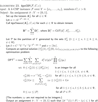
Algorithm 10. _ApxMatrix(A, C, ε)

Input: A 0/1 matrixAof size_m×_n, numbers_{C, ε >}0. Output: A sequence of cut matrices.

1. SetA0=A.

2. Forj= 0,1,2, . . . , κdo

3. Compute setsSj+1, Tj+1of sizes|Sj+1| ≥m/2,|Tj+1| ≥n/2such that |Aj(Sj+1, Tj+1)| ≥α0Aj2/4.

4. If|Aj(Sj+1, Tj+1)|< α0εmnp/4andj≥1, then

output the cut matricesD1, . . . ,Djand halt.

5. else

compute

dj+1= A_|Sj(Sj+1, Tj+1)

j+1||Tj+1| ,

setD_j+1=CUT(dj+1, Sj+1, Tj+1), and letAj+1=Aj−Dj+1.

6. Output “failure.”

Fig. 1.Pseudocode for_ApxMatrix.

satisfy A(_{X1, X2, . . . , Xk}) = A₂. This yields the assertion, as _{X1, . . . , Xk} are unions of classes ofR_{1, . . . ,}R_k.

3. Approximating and partitioning 0/1 matrices and graphs. This sec-tion contains the proofs of Theorem 1 and Corollaries 2 and 3. In secsec-tion 3.1 we discuss the algorithm ApxMatrix in Figure 1 and outline the proof of Theorem 1. Section 3.2 contains the proof of a proposition that is needed to establish Theorem 1. Furthermore, section 3.3 deals with the proof of Corollary 2, and section 3.4 features the proof of Corollary 3.

3.1. The algorithm _ApxMatrix for Theorem 1. Let_{C >}1 and 0 _{< ε <} 1₂. Moreover, let_α0 be the constant from Theorem 7, and set

(6) _κ=513C

2

ε2α20 , γ

= εα0

210(κ+1)_C.

Throughout this section we assume thatAis a 0/1 matrix of size_m×_n.

In order to approximateA by a sum of cut matrices,ApxMatrixproceeds in up to_κ+ 1 rounds_j= 0_,1_{, . . . , κ}, each time generating a new cut matrixD_j+1. Hence, in iteration _j A_j = A−j_i=1D_j is the remaining “error term” that results from approximating A by j_i=1D_j. If _j = 0, then of course A₀ = A is just the input matrix. Thus, the goal is to eventually achieve an approximationD₁+· · ·+D_j such that the “error term” A_j has a sufficiently small cut norm (namely, cut norm less than_εA₂).

To this end, step 3 computes sets _{Sj+1, Tj+1} of rows and columns such that

|A_j(_{Sj+1, Tj+1})| is a good approximation of the cut norm of A_j. More precisely, we have|A_j(_{Sj+1, Tj+1})| ≥_α0A_j2/4, where _α0 is the constant from Theorem 7. Hence, if|A_j(_{Sj+1, Tj+1})|_{< α0εmnp/}4, then we are done because

(7) A−(D₁+· · ·+D_j)₂=A_j2≤_εmnp=_εA_2.

By contrast, if |A_j(_{Sj+1, Tj+1})| ≥ _α0εmnp/4, then _{Sj+1, Tj+1} witness a set of rows/columns on whichD₁+· · ·+D_j does not yet provide a good enough approxi-mation. Therefore, step 5 adds a further “patch”D_j+1, which is a cut matrix whose value on _Sj+1 ×_Tj+1 is just the average _dj+1 of A_j over that square. Note that dj+1 may be negative. This construction ensures thatAj+1(Sj+1, Tj+1) = 0 and thus remedies the discrepancy witnessed by_{Sj+1, Tj+1}.

If the algorithm outputs cut matricesD_{1, . . . ,}D_j, then (7) guarantees thatD₁+

· · ·+D_j approximatesA sufficiently well. Hence, in order to establish Theorem 1, we need to prove the following:

(a) Step 3 of ApxMatrixcan be implemented by a polynomial time algorithm. (b) IfA is (_{C, γ})-bounded, then the halting condition in step 4 will be satisfied

for some 1≤_j≤_κ.

The following proposition takes care of (a).

Proposition 11. In step3,S_j+1, T_j+1 can be computed in timepoly(mn).

Proof. We apply the algorithm from Theorem 7 to the _m×_n matrix A_j. The algorithm has running time poly(_nm) and outputs sets _{Sj+1, Tj+1} such that

|A_j(_{Sj+1, Tj+1})| ≥ _α0A_j2. The problem is that Theorem 7 does not guarantee a lower bound on the sizes of these sets, while it is required that|_Sj+1| ≥_m/2 and

|Tj+1| ≥n/2. To resolve this issue we proceed as follows. Case1: |_Sj+1| ≥_m/2. We just let_Sj+1=_Sj+1. Case2: |_Sj+1|_{< m/}2. Since

A_j([_m]_{, Tj+1}) =A_j(_{Sj+1, Tj+1}) +A_j([_m]\_{Sj+1, Tj+1})_,

we have

max{|A_j([_m]_{, Tj+1})|_,|A_j([_m]\_{Sj+1, Tj+1})|} ≥ |A_j(_{Sj+1, Tj+1})|_/2

≥α0A_j2/2_. (8)

Let_Sj+1= [_m] if|A_j([_m]_{, Tj+1})| ≥ |A_j([_m]\_{Sj+1, Tj+1})|, and set_Sj+1= [_m]\_Sj+1 otherwise. Then (8) ensures that|A_j(_{Sj+1, Tj+1})| ≥_α0A_j2/2 and the assumption

|Sj+1|< m/2 implies|Sj+1| ≥m/2.

In order to obtain_Tj+1 we proceed similarly. Case1: |_Tj+1| ≥_n/2. Let_Tj+1=_Tj+1. Case2: |_Tj+1|_{< n/}2. We have

max{|A_j(_Sj+1,[_n])|_,|A_j(_Sj+1,[_n]\_Tj+1)|} ≥ |A_j(_{Sj+1, Tj+1})|_/2

≥α0A_j2/4_.

Setting either _Tj+1 = [_n] or _Tj+1 = [_n]\_Tj+1 thus yields a set of size at least _n/2 such that|A_j(_{Sj+1, Tj+1})| ≥_α0A_j2/4.

The overall running time is clearly polynomial in_m·_n.

The following proposition establishes (b) above. We defer its proof to section 3.2. Proposition 12. _{If A is (C, γ)-bounded, then there is 1} ≤ _j ≤ _{κ such that}

|A_j(_{Sj+1, Tj+1})|_{< α0εmnp/}4.

Proof of Theorem 1. Proposition 11 ensures that each iteration of steps 3–5 runs in time Π(_mn) for some polynomial Π. Hence, the total running time of ApxMatrixis bounded by_κ·Π(_mn), as claimed. Furthermore, Proposition 12 ensures that on a (_{C, γ})-bounded input A _ApxMatrixwill output a sequence D_{1, . . . ,}D_j of cut matrices for some 1 ≤ _j ≤ _κ. Finally, (7) entails that this sequence satisfy

3.2. Proof of Proposition 12. Throughout this section we assume thatAis a (_{C, γ})-bounded_m×_nmatrix. We let _{κ, γ}be as in (6) and set_γ = 2κ_γ. The proof is by contradiction. That is, we assume that

(9) |A_j(_{Sj+1, Tj+1})| ≥_α0εmnp/4 for all 0≤_j ≤_κ.

We are going to construct families (A_j)_1≤j≤κ and (D_j)_1≤j≤κ of matrices such that the matrices D_j, A_j are “close” to D_j, A_j in the cut norm and such that we can use the boundedness condition to derive upper and lower bounds on the Frobenius norms ofA_j for 1 ≤_j ≤_κ. These bounds on the Frobenius norm will then yield a contradiction to (9).

The matrices D_j, A_j are defined as follows. Due to assumption (9), step 4 of ApxMatrixdoes not terminate the algorithm for any_j≤_κ. Hence, steps 2–5 construct sets_{S1, . . . , Sκ}of rows and_{T1, . . . , Tκ}of columns. LetSbe the partition of the set [_m] of row indices generated by_{S1, . . . , Sκ}. Similarly, letT be the partition of the column set [_n] generated by _{T1, . . . , Tκ}. Then both S and T have at most 2κ classes. We define

R0=

S∈S:|S|<γm

S, C0=

T∈T:|T|<γn

T

to be the sets that comprise the “small” classes of the partitionsS_,T.

Fact 13. _{We have}|_R0| ≤_{γm and}|_C0| ≤_γn.

Proof. The definition of_R0 ensures that|_R0| ≤ |S| ·_γm. SinceS has at most 2κ classes, we obtain|_R0| ≤2κ_γm=_γm. Similarly, |_C0| ≤2κ_γn=_γn.

LetA₀=A be the matrix obtained from Aby replacing all rows in_R0 and all columns in _C0 by 0. In addition, define inductively _Sj =_Sj\_R0 and _Tj =_Tj\_C0 and

dj+1 =

A_j(_{Sj+1, Tj+1})

|S_j+1||T_j+1| , D

j+1 = CUT(Sj+1, Tj+1, dj+1), Aj+1=Aj−Dj+1.

LetSbe the partition of [_m]\_R0generated by_{S1, . . . , Sκ}, and letTbe the partition of [_n]\_C0 generated by_{T1, . . . , Tκ}.

Fact 14. _{All classes of}S _(resp., T_{) have size at least γm(resp., γn).}

Proof. LetS be the partition of [_m]\_R0that consists of all classes _S∈ S such that _S ⊂[_m]\_R0. Then each class of S has size at least_γm, because_R0 contains all classes of S that are smaller than _γm. Moreover, each of the sets _{S1, . . . , Sκ} is a union of classes ofS. Hence,Sis coarser thanS, and thus each class ofScontains a class ofS. Therefore, each class of S has size at least _γm. The same argument applies toT.

The key step is to derive the following bound on the Frobenius norm ofA_j.

Lemma 15. For all 1≤j≤κwe haveA_j2

F ≤ A2F(1−j·α20ε2p/256). The proof of Lemma 15 requires some preparations: we need to bound the cut normsA−A₂ (Lemma 16), D_j−D_j2 (Corollary 18), and A_j−A_j2 (Corollary 19).

Lemma 16. We have A−A₂≤A(R0,[n]) +A([m], C0)≤2Cγmnp.

the rows_R0 and the columns_C0 by 0. Therefore,A−A is a 0_/1 matrix, whose cut norm equals the number of ones it contains. Hence,

A−A₂= (A−A)([_m]_,[_n]) =A(_R0,[_n]) +A([_m]_{, C0})−A(_{R0, C0})

≤A(_R0,[_n]) +A([_m]_{, C0})_.

To show thatA(_R0,[_n])≤_Cγmnpwe consider two cases. Recall that we are assum-ing thatAis (_{C, γ})-bounded.

Case1: |_R0| ≥_γm. Because the boundedness condition implies

A(_R0,[_n])≤_C|_R0|_np,

Fact 13 entailsA(_R0,[_n])≤_Cγmnp.

Case 2: |_R0|_{< γm}. Let _R0⊂_R0 ⊂[_m] be a superset of_R0 of size_γm. Since Ais a 0_/1 matrix, we haveA(_R0,[_n])≤A(_R0,[_n]). Moreover, as|_R0| ≥_γm, we can apply the boundedness condition to getA(_R0,[_n])≤_C|_R0|_np≤_Cγmnp, as desired.

The same argument yieldsA([_m]_{, C0})≤_Cγmnpand thus the assertion. To show that the matricesD_j,D_j are close in the cut norm, we need a bound on the coefficients_dj from step 5 of ApxMatrix.

Lemma 17. |_dj| ≤₂j_{Cp for all1}≤_j≤_κ.

Proof. The proof is by induction on_j. Since the matrixA=A₀is (_{C, γ})-bounded and|_S0| ≥ m₂ and|_T0| ≥ n₂ (cf. step 3), we haveA₀(_{S1, T1})≤_C|_S0||_T0|_p. Hence,

d1= A0(S1, T1)

|S1||T1| ≤Cp.

Furthermore, assuming that|_di| ≤2i_Cpfor all_i≤_j, we obtain

|A_j(_{Sj+1, Tj+1})|=

A0(Sj+1, Tj+1)−

j

i=1

D_i(_{Sj+1, Tj+1})

=

A0(Sj+1, Tj+1)−

j

i=1

di|Sj+1∩Si| |Tj+1∩Ti|

≤ |A₀(_{Sj+1, Tj+1})|+|_Sj+1||_Tj+1|

j

i=1

|di| [triangle inequality]

≤ |A₀(_{Sj+1, Tj+1})|+|_Sj+1||_Tj+1|

j

i=1

2i_Cp [by induction]

≤ |A₀(_{Sj+1, Tj+1})|+ (2j+1−1)|_Sj+1||_Tj+1|_Cp. (10)

As A₀ is (_{C, γ})-bounded and |_Sj+1| ≥ m₂ and |_Tj+1| ≥ n₂ by the construction in step 3, we have the bound |A₀(_{Sj+1, Tj+1})| ≤ _Cp|_Sj+1||_Tj+1|. Thus, (10) yields

|dj+1|=|A_j(_{Sj+1, Tj+1})|_/(|_Sj+1||_Tj+1|)≤2j+1_Cp. Corollary 18.

1. For all1≤_j≤_κwe haveD_j−D_j2≤28j_Cγmnp.

Proof. We prove the first assertion by induction on_j. The definitions of_dj and dj imply that

_d

j−dj=

A_j−1(_{Sj, Tj})

|S_j||T_j| −

A_j−1(_{Sj, Tj})

|Sj||Tj|

= |Sj||Tj|A

j−1(Sj, Tj)− |Sj||Tj|Aj−1(Sj, Tj) |Sj||Sj||Tj||Tj|

≤ Aj−1(Sj, T_|j)−Aj−1(Sj, Tj)

S_j||T_j| +

(|_Sj||_Tj| − |_Sj||_Tj|)A_j−1(_{Sj, Tj})

|Sj||Sj||Tj||Tj|

+A

j−1(Sj, Tj)−Aj−1(_{Sj, Tj})

|Sj||Tj| .

(11)

To bound the denominators, remember from step 3 that |_Sj| ≥ m₂ and |_Tj| ≥ n₂. Furthermore, as_Sj =_Sj\_R0 and|_R0| ≤_{γm < m/}4 by Fact 13, we have |_Sj| ≥ m₄. Similarly,|_Tj| ≥n₄. Hence, (11) yields

_d

j−dj≤16(mn)−1(Aj−1(Sj, Tj)−Aj−1(Sj, Tj))

+ 64(_mn)−2|A_j−1(_{Sj, Tj})|(|_R0||_C0|+|_R0||_Tj|+|_Sj||_C0|) + 16(_mn)−1A_j−1(_{Sj, Tj})−A_j−1(_{Sj, Tj})_.

(12)

To start the induction, we evaluate the term on the right-hand side (r.h.s.) of (12) for_j= 1. Since _S1 =_S1\_R0and_T1 =_T1\_C0, and asA₀ is obtained fromA =A by replacing the rows_R0and the columns_C0by 0, we haveA₀(_{Sj, Tj}) =A₀(_{Sj, Tj}). Hence, the third term on the r.h.s. of (12) vanishes. Moreover, asA₀is a 0/1 matrix, we have

A₀(_{S1, T1})−A₀(_{S1, T1}) =A₀(_S1∩_{R0, T1}) +A₀(_{S1, T1}∩_C0)

−A₀(_S1∩_{R0, T1}∩_C0)

≤A([_m]_{, C0}) +A(_R0,[_n])≤2_Cγmnp [by Lemma 16]_.

Hence,

(13) 16(_mn)−1(A_j−1(_{Sj, Tj})−A_j−1(_{Sj, Tj}))≤32_γCp.

Further,A₀(_{S1, T1})≤A₀([_m]_,[_n]) =_mnp. As|_R0| ≤_γmand|_C0| ≤_γnby Fact 13, we get

(14) 64(_mn)−2|A_j−1(_{Sj, Tj})|(|_R0||_C0|+|_R0||_Tj|+|_Sj||_C0|)≤64_γ(2+_γ)_p≤192_γp.

Plugging (13) and (14) into (12), we get |_d1−_d1| ≤ _Cγp(32 + 192) = 224_Cγp. Consequently,

D₁−D₁₂≤ |_d1−_d1|_mn≤28_Cγmnp,

as claimed.

Now let 2≤_j≤_κ, and assume that

For any two sets_S⊂[_m],_T ⊂[_n] we have

|A_j−1(_{S, T})|=

A(S, T) +

j−1

i=1

D_i(_{S, T})

≤A(_{S, T}) +

j−1

i=1

|D_i(_{S, T})| [triangle inequality]

≤A(_{S, T}) +

j−1

i=1

|di||S||T|

≤A(_{S, T}) +

j−1

i=1

2i_Cp· |_S||_T| [by Lemma 17]

≤A(_{S, T}) + (2j−1)_Cp|_S||_T|_. (16)

Therefore,

A_j−1(_{Sj, Tj})−A_j−1(_{Sj, Tj})

=|A_j−1(_{Sj, Tj}∩_C0) +A_j−1(_Sj∩_{R0, Tj})−A_j−1(_Sj∩_{R0, Tj}∩_C0)|

≤|A_j−1(_{Sj, Tj}∩_C0)|+|A_j−1(_Sj∩_{R0, Tj})|+|A_j−1(_Sj∩_{R0, Tj}∩_C0)|

≤A(_{Sj, Tj}∩_C0) +A(_Sj∩_{R0, Tj}) +A(_Sj∩_{R0, Tj}∩_C0)

+ (2j−1)_Cp(|_Sj||_Tj∩_C0|+|_Sj∩_R0||_Tj|+|_Sj∩_R0||_Tj∩_C0|)

≤A(_R0,[_n]) +A([_m]_{, C0}) + (2j−1)_Cp(|_R0|_n+_m|_C0|)_. (17)

SinceA(_R0,[_n]) +A([_m]_{, C0})≤2_Cγmnpby Lemma 16 and|_R0| ≤_γm,|_C0| ≤_γn by Fact 13, (17) yields

A_j−1(_{Sj, Tj})−A_j−1(_{Sj, Tj})≤2j+1_γCmnp. (18)

Moreover, asAis a 0_/1 matrix, (16) yields

|A_j−1(_{Sj, Tj})| ≤A(_{Sj, Tj}) + (2j−1)_Cp|_Sj||_Tj|

≤A([_m]_,[_n]) + (2j−1)_Cmnp≤2j_Cmnp. (19)

Furthermore,

A_j−1(_{Sj, Tj})−A_j−1(_{Sj, Tj})=

j−1

i=1

D_i(_{Sj, Tj})−D_i(_{Sj, Tj})

≤ j−1

i=1

D_i(_{Sj, Tj})−D_i(_{Sj, Tj})

≤ j−1

i=1

D_i−D_i2

≤Cγmnp

j−1

i=1

28j [by (15)]