http://wrap.warwick.ac.uk/
Original citation:
Ludvig, Elliot A., Sutton, Richard S. and Kehoe, E. James. (2008) Stimulus
representation and the timing of reward-prediction errors in models of the dopamine
system. Neural Computation, Volume 20 (Number 12). pp. 3034-3054. ISSN 0899-7667
Permanent WRAP url:
http://wrap.warwick.ac.uk/58755
Copyright and reuse:
The Warwick Research Archive Portal (WRAP) makes this work by researchers of the
University of Warwick available open access under the following conditions. Copyright ©
and all moral rights to the version of the paper presented here belong to the individual
author(s) and/or other copyright owners. To the extent reasonable and practicable the
material made available in WRAP has been checked for eligibility before being made
available.
Copies of full items can be used for personal research or study, educational, or
not-for-profit purposes without prior permission or charge. Provided that the authors, title and
full bibliographic details are credited, a hyperlink and/or URL is given for the original
metadata page and the content is not changed in any way.
Publisher’s statement:
Ludvig, Elliot A., Sutton, Richard S. and Kehoe, E. James. (2008) Stimulus
representation and the timing of reward-prediction errors in models of the dopamine
system. Neural Computation, Volume 20 (Number 12). pp. 3034-3054. ISSN 0899-7667
© MIT Press, 2008.
http://dx.doi.org/10.1162/neco.2008.11-07-654
A note on versions:
The version presented in WRAP is the published version or, version of record, and may
be cited as it appears here.
Stimulus Representation and the Timing of Reward-Prediction
Errors in Models of the Dopamine System
Elliot A. Ludvig
Richard S. Sutton
University of Alberta, Edmonton, Alberta T6G 2E8, Canada
E. James Kehoe
University of New South Wales, Sydney 2052, New South Wales, Australia
The phasic firing of dopamine neurons has been theorized to encode a reward-prediction error as formalized by the temporal-difference (TD) algorithm in reinforcement learning. Most TD models of dopamine have assumed a stimulus representation, known as the complete serial com-pound, in which each moment in a trial is distinctly represented. We introduce a more realistic temporal stimulus representation for the TD model. In our model, all external stimuli, including rewards, spawn a series of internal microstimuli, which grow weaker and more diffuse over time. These microstimuli are used by the TD learning algorithm to generate predictions of future reward. This new stimulus represen-tation injects temporal generalization into the TD model and enhances correspondence between model and data in several experiments, includ-ing those when rewards are omitted or received early. This improved fit mostly derives from the absence of large negative errors in the new model, suggesting that dopamine alone can encode the full range of TD errors in these situations.
1 Introduction
For any organism, learning to find good things (rewards) while avoid-ing bad thavoid-ings (punishers) is a key mechanism for survival. In the mam-malian brain, much reward-related information passes through dopamin-ergic pathways. For example, dopamine neurons produce response bursts to unexpected rewards, as well as to cues that reliably predict upcoming rewards. This pattern of phasic firing has been interpreted as encoding a reward-prediction error corresponding to the temporal-difference (TD) er-ror prominent in reinforcement-learning algorithms (Montague, Dayan, & Sejnowski, 1996; Schultz, Dayan, & Montague, 1997). This error, in turn, is
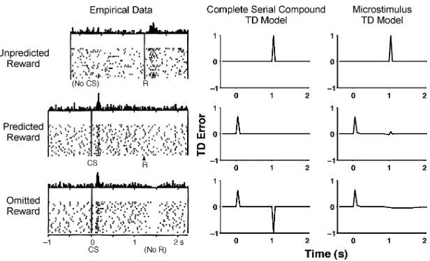
Figure 1: Summary of empirical data and simulation results. Empirical data from monkey dopamine neurons (left column), simulation results from the TD model with complete-serial-compound stimulus representation (middle col-umn), and results from our new TD model with microstimuli (right column). From top to bottom, data and simulations are presented for unpredicted re-wards, predicted rere-wards, and the omission of predicted rewards. See text for full simulation details. (Data are from Schultz et al., 1997. Reprinted with permission.) In empirical data figures, CS= conditioned, reward-predicting stimulus and R=reward; dots represent firing of individual neurons; and the bars are a histogram of that firing.
important for learning predictions of future rewards and selecting appro-priate responses. Though the exact role of dopamine in reward is still de-bated (for an alternative viewpoint, see Berridge, 2007), the reinforcement-learning model of dopaminergic function has helped yield numerous in-sights into learning and decision making (Montague, 2006; Montague, Hy-man, & Cohen, 2004) as well as disorders like Parkinson’s disease (Frank, Seeberger, & O’Reilly, 2004; Shohamy, Myers, Grossman, Sage, & Gluck, 2005) and drug addiction (Redish, 2004; Redish, Jensen, Johnson, & Kurth-Nelson, 2007). In this letter, we extend these TD models to include a more re-alistic temporal stimulus representation. This new representation suggests how temporal generalization should occur, thereby generating testable em-pirical predictions as well as considerably improving the TD model’s fit with existent dopamine data.
with corresponding simulations from the basic TD model and our new microstimulus TD model. First, following unpredicted rewards, dopamine neurons show a burst of responding, and there is a strong, positive reward-prediction error in the models (top row). Second, when a neutral cue reliably predicts the upcoming reward, the increased firing after the now-expected reward gradually disappears, and instead, a response burst begins to follow the earliest cue for that reward (middle row). Third, after learning, if an expected reward is omitted, there is a decrease in the firing rates of the dopamine neurons and a corresponding negative TD error in the models around the time when reward would ordinarily have been received (bottom row; data are from Schultz et al., 1997).
All TD models of dopamine work by assuming that the system learns a value for each time step in a trial. These TD models attempt to learn an estimate of the true value V∗, which is equal to the expected cumulative sum of discounted future reward:
Vt∗=E
∞
k=1
γk−1r
t+k
, (1.1)
wherertis the reward at time steptandγ is a discount factor that weights
immediate rewards more heavily than distant rewards. This ideal value is the cumulative sum of all future discounted rewards and thus serves as a prediction of expected future reward at a given time point. With per-fect knowledge of the environment, including state transition probabilities and the reward function, the value could be calculated directly through dynamic programming techniques (Sutton & Barto, 1998). In the absence of such information, however, the value must be estimated. One method for estimating the value is the TD algorithm, whereby an error termδt is
calculated based on thetemporal differenceof the current discounted value (γVt) and the previous value (Vt−1), taking into account the reward received along the way (rt):
δt=rt+γVt−Vt−1. (1.2)
conditioning using TD learning (Desmond & Moore, 1988; Sutton & Barto, 1981, 1990).
Though capturing a wide range of dopamine neuron behavior, these reinforcement-learning models have not dealt adequately with situations when reward timing is varied. The case of reward omission illustrates this problem. After learning, if a reward is omitted, then there is a small but extended reduction in firing rate around the time reward would ordinar-ily have been delivered (see Figure 1). The complete-serial-compound TD model indeed predicts a negative error at the time reward was expected, but this error occurs exactly at that usual time of reward and is even larger than the positive error earlier in the trial. In fact, the actual decrease in dopamin-ergic firing covers a greater temporal extent and a smaller maximal decrease than the corresponding TD error (Schultz et al., 1997). The durations of these pauses in dopamine activity are modulated by the magnitude of negative reward-prediction error, a recent observation that eludes the explanatory net of all previous TD models (Bayer, Lau, & Glimcher, 2007). A similar problem arises for this basic TD model when an expected reward is re-ceived early (Hollerman & Schultz, 1998; see Figure 7 below). Under those conditions, dopamine neurons burst following the early reward and show little change in firing rates around the time reward is ordinarily received. The basic TD model does generate a positive TD error at the time of early reward, but also produces a large negative error exactly at the usual time of reward.
These discrepancies between model and data can mostly be attributed to the choice of the complete serial compound as the temporal stimulus representation in the basic TD model. Given the noisy time perception ob-served in animals during conditioning (Gibbon, 1977; Lejeune & Wearden, 2006; Smith, 1968; Staddon & Cerutti, 2003), this assumption of a perfect clock is too strong. From the initial publications that discussed the relation-ship between dopamine and TD learning (Montague et al., 1996; Schultz et al., 1997), the complete serial compound was recognized as unrealistic but has yet to be adequately replaced. Several attempts have been made to extend or modify the TD model to contend with these problematic neu-rophysiological data, including incorporating resets of the delay line (Suri & Schultz, 1998, 1999), devising alternative learning rules (Brown, Bullock, & Grossberg, 1999; O’Reilly, Frank, Hazy, & Watz, 2007), and switching to partially observable, semi-Markov dynamics (Daw, Courville, & Touretzky, 2006).
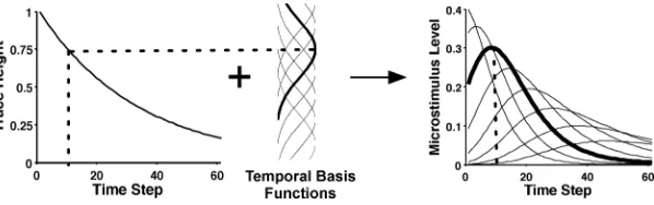
Figure 2: Stimulus encoding by the microstimuli. From left to right, the stimu-lus trace, basis functions, and resulting microstimustimu-lus levels are displayed. The decaying stimulus trace is approximated by a series of basis functions whose receptive fields are evenly spread across the possible trace height. The decreas-ing, nonlinear time course of the trace results in microstimuli that get shorter and wider with time. For illustrative purposes, a single basis function (middle) and approximately corresponding microstimulus (right) have been darkened.
basic TD model produce a more realistic computational framework that accords better with the empirical data.
2 The Microstimulus TD Model
2.1 Stimulus Representation. The primary innovation of our model is the introduction of a more sophisticated temporal stimulus representation for use with the TD learning rule. Figure 2 depicts how this stimulus repre-sentation is constructed. In the model, the onset of any stimulus, including sensory cues and rewards, is assumed to leave behind a decaying memory trace of that stimulus (left panel). The trace is then encoded by a series of temporal basis functions or receptive fields evenly spaced along the trace height (middle panel). Each basis function encodes how close the current trace is to the center of that receptive field. This proximity measure be-comes a feature or microstimulus, which is then input to the TD learning algorithm. In effect, the memory trace is not a single, coherent whole, but is made up of many separate elements with different temporal dynamics.
temporal stimulus representation in our model is, in effect, a relaxation of the assumption of perfectly discrete and distinct temporal features in the complete serial compound. By using overlapping basis functions, we create more graded temporal features that allow for temporal generalization be-tween neighboring time points. All stimuli, including rewards, are assumed to be represented by separate stimulus traces, each with a corresponding set of microstimuli.
For the basis functions, we chose simple gaussians:
f(y, µ, σ)= √1 2πexp
−(y−µ)2 2σ2
, (2.1)
where y is the input value (i.e., trace height) with µ the center and σ the width of each basis function. The basis functions were uniformly dis-tributed across the height of the memory trace. The selection of the gaussian as the basis function was likely not strictly necessary for this type of model. Other functions, including the traces in spectral timing theory (Grossberg & Schmajuk, 1989) and the behavioral states in the learning to time theory (LeT; Machado, 1997), may produce similar results. We chose this stimulus representation for simplicity and ease of calculation. Given the basis func-tions, the level of theith microstimulusxt(i), at timet, is determined by the
corresponding trace heights:
xt(i)= f(yt,i/m, σ)yt, (2.2)
where f is the basis function defined above in equation 2.1 andmis the total number of microstimuli per stimulus. The trace heightytwas set to 1
at stimulus onset and decreased exponentially, controlled by a single decay parameter, which was fixed at 0.985 per time step for all stimuli.
2.2 Learning Algorithm. The model learns through the linear TD(λ) algorithm(Sutton, 1988). At each time step, the estimated value is deter-mined by
Vt =wtTxt= n
i=1
wt(i)xt(i), (2.3)
wherext is the vector of microstimulus levelsxt(i),wt is a corresponding
vector of adjustable weightswt(i), andnis the total number of all
generate a TD error (δt) at each time step (see equation 1.2). This TD error is
then used to update the weight vector based on the following update rule,
wt+1=wt+αδtet, (2.4)
where α is a step-size parameter and et is a vector of eligibility trace levels (Sutton & Barto, 1998), which together help determine the speed of learning. The eligibility traces represent a decaying window of plasticity during which a microstimulus can be learned about (i.e., its weights can be adjusted). Each microstimulus has its own corresponding eligibility trace, which continuously decays, but accumulates whenever that microstimulus is present,
et+1=γ λet+xt, (2.5)
whereγ is the discount factor as above andλis a decay parameter that determines the plasticity window. The earliest TD models of dopamine all used implicit, one-step eligibility traces (Montague et al., 1996; Schultz et al., 1997), whereby only weights on stimulus components active on the previous time step were updated (i.e., effectively λ = 0), though more recent work has occasionally incorporated multistep (nonzero) eligibility traces (see Pan, Schmidt, Wickens, & Hyland, 2005).
Our model is completely defined by equations 1.2 and 2.1 to 2.5, the two memory trace parameters (initial height and decay rate), and five additional parameters, which were fixed at the following values for all simulations:
λ =0.95, α= 0.01, γ = 0.98, n= 50, and σ =0.08. We used this single set of parameters in an attempt to establish a general correspondence with available empirical findings rather than conducting a set of curve-fitting exercises. In all simulations, 20 time steps were interpreted as a unit of 1 s, and an intertrial interval of 500 time steps separated the onsets of all trials. Preliminary simulations in which we varied these parameters revealed that the general pattern of simulated outcomes was consistent across these manipulations.
3 Results
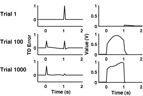
Figure 3: Simple acquisition simulations. TD error (δ; left column) and value (right column) at each time step on trials 1, 100, and 1000. A cue occurred at time 0, and reward consistently followed exactly 1 s (20 time steps) later.
3.1 Simple Acquisition. During simple acquisition, monkeys are pre-sented with a cue that reliably predicts reward a short time later. At first, their midbrain dopamine neurons show a phasic burst of firing after the reward. Once the cue-reward contingency is well learned, these neurons fire after the earliest cue that predicts reward, but show no deviation from baseline activity when reward is received. Intermediate stages of learning show a mixture of these two end points with midsized responding at both cue onset and reward.
Figure 3 illustrates the behavior of our microstimulus model during simple acquisition (see also Figure 1). The three rows present different stages of training, from the first trial (top row) to near-asymptotic performance after 1000 trials (bottom row). The left column depicts the TD error (δ), and the right column depicts the estimated value (V). In all simulations, the cue was presented at time 0, and reward was delivered 1 s later, on time step 20. At the onset of training, the estimated value was 0, and when the (unexpected) reward was delivered, there was a large, positive TD error. Notice how there was a small upward blip in the estimated value after the reward was received, even on the first trial. This blip is quite informative as to how our model learns: after the reward was received, there was a large, positive TD error, and the weights on eligible microstimuli were duly updated. These microstimuli, however, did not turn off immediately, and thus, on the very next time step, there was an expectation of reward, and the estimated value was no longer 0.
Figure 4: Reward omission simulations. TD error (δ; left column) and value (right column) at each time step for an omission trial after 1000 trials of training. A cue occurred at time 0, and reward usually followed exactly 1 s (20 time steps) later.
Notice how there was little TD error at intermediate time points or any visible ramp—a point of contention in the literature for both the empirical data and theoretical models (Fiorillo, Tobler, & Schultz, 2003, 2005; Niv, Duff, & Dayan, 2005; O’Reilly et al., 2007; Pan et al., 2005). Finally, by the end of training, the TD error at cue onset remained, but the error at re-ward delivery had virtually disappeared, though not entirely, as the model learned to correctly predict the occurrence of reward. This full pattern of results roughly matches earlier TD models and corresponds nicely with the empirical data (Schultz et al., 1997; see Figure 1).
Figure 5: Net reward predictions. Estimated value generated individually by the cue microstimuli (left column), the reward microstimuli (middle column), and their combination (right column) after 1000 trials of training. Arrows indi-cate the delivery of the cue or conditioned stimulus (CS) at time 0 and reward (R) exactly 1 s (20 time steps) later. Note that the estimated value due to the cue microstimuli is identical to an omission trial and the net estimated value due to the combination of microstimuli is identical to a rewarded trial.
match to empirical data over the basic TD model, however, is independent of particular parameter settings.
The value or reward prediction (see Figure 4, right panel, and see Figure 5) helps explain why the microstimulus model produces this result. Within a trial, at the moment when the reward was omitted, the estimated value did not immediately disappear because the cue microstimuli re-mained active even beyond the time of ordinary reward (cf. Figure 2). This continued activity of the cue microstimuli resulted in a positive estimated value on omission trials that persisted past the usual time of reward, and thus a persistent negative error when no reward was received. Ordinarily, on rewarded trials, these same cue microstimuli are also active past reward delivery, but the positive reward prediction thereby generated is countered by large, negative weights on the reward microstimuli, resulting in no net value for the time points following reward.
Figure 5 displays this interaction between the values caused by the indi-vidual stimuli (cues and rewards). After training, the cue alone (right panel) produced a positive value that extended past the usual time of reward; the reward alone (middle panel), however, produced a negative value that com-bined with the cue-induced value to produce the net estimated value (right panel) on rewarded trials. When reward was omitted (see Figure 4), how-ever, the balancing force of the reward microstimuli was absent, and the persistent cue microstimuli generated an unimpeded positive value, which gradually declined as the cue microstimuli fell to 0. The decrease in esti-mated value was small at each time step, repeatedly producing a small neg-ative prediction error until the reward prediction for that trial disappeared. With our microstimulus model, no large negative errors occurred with re-ward omission, nor would any need to be encoded by dopamine neurons.
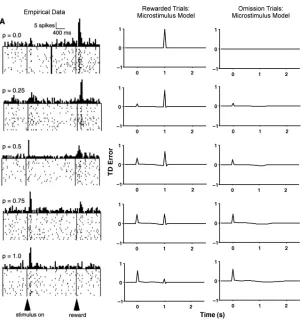
[image:11.432.60.371.71.140.2]Figure 6: Partial reinforcement simulations. Empirical data from a representa-tive monkey dopamine neuron (left column) and simulation results from the microstimulus TD model (right two columns). The empirical data and the first column of simulation results (middle column) show rewarded trials, and the final column shows simulation results for omission trials. Each row depicts a different probability of reward; from top to bottom, these probabilities were 0.00, 0.25, 0.50, 0.75, and 1.00. In the simulations, a cue occurred at 0 s, and reward sometimes followed exactly 1 s (20 time steps) later. Simulated results show the TD error (δ) and are drawn from a single reward or omission trial pre-sented after 500 trials of training with the corresponding probability of reward. (Data are from Fiorillo et al., 2003. Reprinted with permission.)
there was an increase in dopamine neuron firing at cue onset and a corre-sponding decrease in firing at reward delivery. After 500 trials of training, the microstimulus model (middle column) showed a similar pattern of results for rewarded trials. There was a TD error at cue onset that was pro-portional to the probability of reward and a TD error at reward delivery that was inversely proportional to that probability. On omission trials (right column in Figure 6), the model showed a small, temporally extended nega-tive TD error around the usual time of reward. This neganega-tive error was also proportional to the probability of reward and covered a slightly smaller time span (though still extended) with lower reward probabilities.
This pattern of results emerged mostly because the learned value (or predicted future reward) was scaled by the probability of reward. With higher probabilities of reward, the model expected more reward in the fu-ture when the cue was present, leading to a larger jump in value (and TD error) at cue onset, but a smaller reward-prediction error when the reward was actually delivered. When reward was omitted, the value was lower with the smaller probabilities, and the corresponding negative error was shallower and also covered a shorter temporal extent (cf. Bayer et al., 2007). These two facets of the negative error had different causes: the shallower negative error occurred because the value was scaled by reward proba-bility and therefore decreased more slowly. The shorter temporal extent stemmed from the frequency of omission trials; with more frequent nonre-warded trials, the temporal accuracy of the reward prediction on those trials actually improved as the system relied less on the reward microstimuli (see Figure 5) and more on the cue microstimuli alone, resulting in more tempo-rally concentrated negative errors. Even with the repeated reward omission (reward probabilities less than 1.00), our microstimulus model continued to show small, extended negative errors because the chosen microstimulus representation was not complete and a perfectly timed reward prediction could not be learned even at asymptote. Here, too, there were no TD errors at intermediate time points or any visible ramp in the error time course (Fiorillo et al., 2003, 2005; Niv et al., 2005). As suggested by Fiorillo et al. (2005), altering the temporal stimulus representation can indeed eliminate the interim backpropagating TD errors noted by Niv et al. (2005).
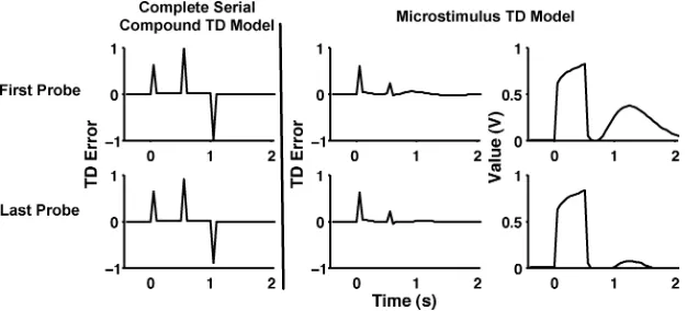
Figure 7: Early reward simulations. TD error (δ) for the complete-serial-compound TD model (left column) and both TD error (δ) and value for the microstimulus TD model (right two columns) for 15 early reward probe trials after 1000 trials of training. A cue occurred at time 0, and reward followed either 0.5 s (probe) or 1 s (nonprobe) later. Simulation results are displayed for the first (top row) and last (bottom row) probes.
the reward and gradually tapered off. As a result, the reduction of the es-timated value at the usual time of reward due to the reward microstimuli should be correlated with how early that reward arrives: the earlier the reward, the smaller the reduction in the estimated value. If the reward comes only moderately early (approximately 90% of the usual interval), there would be little net value at the usual time of reward because there would be strong negative weights on the shortest reward microstimuli. Thus, there would be virtually no TD error and, accordingly, no expected dopamine response. In contrast, very early rewards (approximately 10% of the usual interval) would produce large reward predictions at the usual time of reward because the suppressive effects of the reward microstimuli on the net value would have faded away. Thus, the model predicts an ex-tended, negative TD error in this situation, similar to that expected for and observed on omission trials (see Figure 4). The complete-serial-compound TD model, however, would predict a large negative prediction error at the exact time of reward for both these situations.
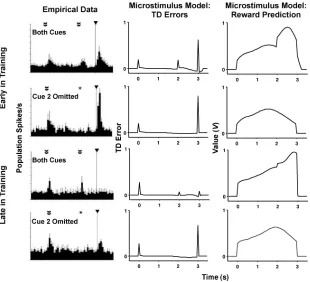
3.5 Multiple Cues. When multiple sequential cues precede reward dur-ing conditiondur-ing, both the TD error and dopamine burst percolate back to the earliest reliable predictor of the reward (Pan et al., 2005; Sutton & Barto, 1981, 1990; see also Kehoe, Schreurs & Graham, 1987). Figure 8 depicts this finding in the empirical data (left column) from rat dopamine neurons (Pan et al., 2005) as well as corresponding simulations from our microstimulus TD model. The top rows present data from early in training (after 50 trials in the simulations), and the bottom rows depict data from late in training (after 1000 trials in the simulations). In the trials with both predictive cues present (first and third rows), there were positive peaks and bursts at the onsets of both cues as well as the reward (though the latter two were muted late in training). Moreover, omitting the second cue (second and fourth rows in Figure 8) produced a drastic increase in neural firing following reward delivery. Finally, early in training (top row), there was response to both the initial cue and the reward, a result taken as evidence for nonzero eligibility traces in the complete-serial-compound TD model (Pan et al., 2005).
Figure 8: Multiple cue simulations. Empirical data (left column) from rat dopamine neurons and TD error (middle column) and value (right column) from microstimulus TD model simulations in an experiment with multiple pre-dictive cues. Two cues (double arrows) were presented in sequence before the reward (single arrow/line); the first cue occurred at time 0 with the second cue and reward usually following 2 and 3 s later, respectively. The top two rows show results from early in training (50 trials in the simulations), and the bottom two rows show results from late in training (1000 trials in the simulations). The first and third rows show results when both cues and the reward were presented. The second and fourth rows show results when the second cue was omitted (indicated with an asterisk). (Data are reprinted from Figure 3 in Pan et al., 2005. Reprinted with permission.)
was omitted, the reward prediction stemming from that cue’s microstimuli was absent, leading to a smaller estimated value at the time of reward (right column) and a larger TD error on reward delivery (middle column).
neither of these parameter choices was necessary. The temporally extended nature of the microstimuli allows the reward prediction to generalize to the first few time points after only a handful of trials. Even with much larger step sizes (α≥.5) and one-step eligibility traces (λ=0), we found qualitatively similar results (simulations not shown). Thus, as Pan et al. (2005) originally suggested, their conclusion about the necessity of nonzero eligibility traces is indeed contingent on the use of the complete-serial-compound stimulus representation; other stimulus representations, such as our microstimuli, provide an alternative mechanism for modeling their data without requiring certain parameter settings.
Our microstimulus model makes a unique, testable prediction about a similar multicue experiment if the training protocol is varied to resemble a blocking experiment (Kamin, 1969; Waelti, Dickinson, & Schultz, 2001). In such an experiment, as in Pan et al. (2005), multiple sequential cues precede reward, but the second, later cue is inserted only after extensive training with the early cue. Other TD models using the complete-serial-compound stimulus representation, including the modified model of Pan et al. (2005), predict blocking of the dopamine response to the second cue (cf. Waelti et al., 2001). In these models, for the sequential two-cue experiment of Pan et al. (2005; see Figure 8), the continued TD error to the second cue occurs because the learning algorithm divides credit for the prediction error equally between the two stimulus components (one from each cue) active during their shared time steps following the onset of the second cue. In the proposed experiment, in contrast, the first cue is pretrained, so the reward is already perfectly predicted when the second cue is introduced. The perfect prediction in the complete-serial-compound model results in no prediction errors, and thus no learning about the second cue and complete blocking. In our microstimulus model, the reward is never perfectly predicted because of the limited temporal resolution of the stimulus representation. The model learns about the second cue to the extent that this second cue improves the temporal accuracy of the reward prediction. Thus, we do not expect this sort of complete blocking effect to exist, except when the cue onsets coincide (Waelti et al., 2001; see also Barnet, Grahame, & Miller, 1993; Kehoe, Schreurs, & Amodei, 1981; Kehoe et al., 1987). According to our model, a dopamine response to the onset of the second cue should emerge, as occurred in the latter stages of the experiment depicted in Figure 8 (Pan et al., 2005).
4 Discussion
several new testable predictions about the behavior of dopamine neurons in experiments with early rewards or multiple sequential cues.
Our microstimulus TD model makes two related theoretical improve-ments over earlier models that rely on the complete serial compound for stimulus representation (e.g., Montague et al., 1996; Schultz et al., 1997). Each of these changes represents a relaxation of certain assumptions from the earlier TD models. Most prominently, we replace the perfect timing of the complete serial compound with graded microstimuli that provide temporal generalization across nearby time points. In addition, we accord these microstimuli to all events in the environment, including rewards, not only those preselected as conditioned stimuli. We have shown how these refined assumptions improve the model’s correspondence to extant data in a variety of experiments while retaining the simple explanatory power that TD models provide.
The microstimuli in the model, though strictly deterministic, capture one potential source of timing noise: that caused by generalization across nearby time points within a single trial. This temporal generalization could be regarded as a limitation of the sensory temporal perception or an effective strategy for dealing with a noisy world (where perfectly fixed intervals of the sort that dominate these experiments are quite rare). The microstimuli, however, do not address the further question of how to model trial-to-trial variability in timed responding, an issue of considerable importance in the animal learning literature (see Gibbon, 1977; Lejeune & Wearden, 2006; Staddon & Cerutti, 2003). The published literature on dopamine neuron responding does not, to our knowledge, contain data that would adequately constrain further assumptions about trial-to-trial timing stochasticity. We expect that future theoretical and empirical efforts will shed further light on this topic.
Although the earliest TD models of dopamine relied on a complete serial compound for the temporal stimulus representation (Montague et al., 1996; Schultz et al., 1997; Sutton & Barto, 1990), several subsequent models have also attempted to replace those early representational assumptions. For ex-ample, Suri and Schultz (1998, 1999) present a model that uses a sequence of broadening components to represent stimuli. On the surface, these stimu-lus components resemble the microstimuli of our model but serve a wholly different functional role. In their model, learning occurs only when a par-ticular component is descending; the model is constrained so that only one component can be descending on each time step, thus creating, in effect, a complete serial compound and being bound by the limitations of that rep-resentation. Our stimulus representation more closely resembles the traces in spectral timing theory (Grossberg & Schmajuk, 1989) and the behavioral states of the learning to time theory (LeT; Machado, 1997) than the stimulus components in the Suri and Schultz (1998, 1999) model.
More recently, Daw et al. (2006) addressed many of the same empir-ical lacunae in the reinforcement learning and dopamine story with a computational model based on partial observability and semi-Markov dy-namics. Their theory, though elegant and comprehensive, requires a full world model for implementation, thereby losing much of the explanatory force that comes from the simple, mechanistic, incremental account of the dopaminergic system provided by TD models. Our microstimulus theory sticks much more closely to the established TD models, but makes signifi-cant changes in the stimulus representation.
Several recent discussions of the relationship between dopamine and reward-prediction errors have emphasized that the low baseline levels of dopaminergic firing do not allow dopamine to adequately code for negative errors (Bayer & Glimcher, 2005; Bayer et al., 2007; Daw et al., 2006; Niv et al., 2005; Pan et al., 2005). Consequently, dopamine may only encode a rectified reward-prediction error with the negative portion of the error encoded by another neurotransmitter, such as serotonin (Daw, Kakade, & Dayan, 2002). Our results limit the necessity of this additional error-encoding scheme in experiments where rewards are omitted or mistimed. As clearly depicted in Figures 4, 6, and 7, there need be no large negative TD errors in these sit-uations if a form of temporal generalization is introduced into the stimulus representation, as in our model. In partial empirical support of this point, Bayer et al. (2007) recently showed that the phasic pausing in dopamine responding can indeed encode a range of negative reward-prediction er-rors. Though there would still seem to be situations where large, punctate negative reward-prediction errors should exist (perhaps punishment or con-ditioned inhibition), our model limits the range of experimental conditions for which a secondary error-encoding system is required.
of the model. First, the assumption that stimuli are represented as a set of graded microstimuli leads directly to the prediction that strong blocking should occur only when cue onsets coincide. If, after training, a second cue is inserted between the initial cue and reward, this cue would also begin to cause a TD error and should elicit a burst of dopamine responding. Second, the assumption that rewards act like other cues and produce their own microstimuli leads to the prediction that the degree of dopamine responding should depend on the exact timing of an early reward. With a moderately early reward, the model predicts no difference from baseline responding at the usual time of reward, whereas with a very early reward, the model predicts a shallow negative error—similar to that observed on omission trials (see Figure 4). This latter prediction about the effects of very early rewards also differs from that of newer extensions of the TD model; both the models of Suri and Schultz (1999) and Daw et al. (2006) would expect no negative prediction error at the usual time of reward regardless of how early the reward arrives. In the Suri and Schultz (1999) model, the very early reward would still reset the stimulus representation, eliminating all subsequent value for that trial, and in the Daw et al. (2006) model, the very early reward would still precipitate a transition to the ITI state.
Timing is a vital part of any organism’s environment and behavioral repertoire. Predicting when a reward will happen and acting accordingly are crucial for adaptive performance. Our microstimulus TD model provides a solution to part of this temporal prediction problem and matches the empirical data better than the basic, complete-serial-compound TD model. In the future, we expect this temporal stimulus representation to be further refined and used for action selection as part of a model for explaining the conditioning behavior of an entire animal.
Acknowledgments
We thank James Neufeld and Eric Verbeek for technical support and David Silver and Karen Skinazi for editing help. We also thank Michael Frank, Yael Niv, A. David Redish, and Hitoshi Morikawa for reading and commenting on earlier versions of this letter. This research was supported in part by the Informatics Circle of Research Excellence of Alberta, Canada, and the Natural Science and Engineering Research Council of Canada.
References
Barnet, R. C., Grahame, N. J., & Miller, R. R. (1993). Temporal encoding as a determinant of blocking. Journal of Experimental Psychology: Animal Behavior Processes, 19, 327–341.
Bayer, H. M., Lau, B., & Glimcher, P. W. (2007). Statistics of midbrain dopamine neu-ron spike trains in the awake primate.Journal of Neurophysiology, 98, 1428–1439. Berridge, K. C. (2007). The debate over dopamine’s role in reward: The case for
incentive salience.Psychopharmacology (Berl.), 191, 391–431.
Brown, J., Bullock, D., & Grossberg, S. (1999). How the basal ganglia use parallel excitatory and inhibitory learning pathways to selectively respond to unexpected rewarding cues.Journal of Neuroscience, 19, 10502–10511.
Daw, N. D., Courville, A. C., & Touretzky, D. S. (2006). Representation and timing in theories of the dopamine system.Neural Computation, 18, 1637–1677.
Daw, N. D., Kakade, S., & Dayan, P. (2002). Opponent interactions between serotonin and dopamine.Neural Networks, 15, 603–616.
Desmond, J. E., & Moore, J. W. (1988). Adaptive timing in neural networks: The conditioned response.Biological Cybernetics, 58, 405–415.
Fiorillo, C. D., Tobler, P. N., & Schultz, W. (2003). Discrete coding of reward probability and uncertainty by dopamine neurons.Science, 299, 1898–1902. Fiorillo, C. D., Tobler, P. N., & Schultz, W. (2005). Evidence that the delay-period
activity of dopamine neurons corresponds to reward uncertainty rather than backpropagating TD errors.Behavioral Brain Functions, 1, 7.
Frank, M. J., Seeberger, L. C., & O’Reilly, R. C. (2004). By carrot or by stick: Cognitive reinforcement learning in parkinsonism.Science, 306, 1940–1943.
Gibbon, J. (1977). Scalar expectancy theory and Weber’s law in animal timing.
Psychological Review, 84, 279–325.
Grossberg, S., & Schmajuk, N. A. (1989). Neural dynamics of adaptive timing and temporal discrimination during associative learning.Neural Networks, 2, 79–102. Hollerman, J. R., & Schultz, W. (1998). Dopamine neurons report an error in the temporal prediction of reward during learning.Nature Neuroscience, 1, 304–309. Kamin, L. J. (1969). Predictability, surprise, attention and conditioning. In B. A.
Campbell & R. M. Church.Punishment and aversive behavior(pp. 279–296). New York: Appleton-Century-Crofts.
Kehoe, E. J., Schreurs, B. G., & Amodei, N. (1981). Blocking acquisition of the rabbit’s nictitating membrane response to serial conditioned stimuli.Learning and Motivation, 12, 92–108.
Kehoe, E. J., Schreurs, B. G., & Graham, P. (1987). Temporal primacy overrides prior training in serial compound conditioning of the rabbit’s nictitating membrane response.Animal Learning and Behavior, 15, 455–464.
Lejeune, H., & Wearden, J. H. (2006). Scalar properties in animal timing: Conformities and violations.Quarterly Journal of Experimental Psychology, 59, 1875–1908. Machado, A. (1997). Learning the temporal dynamics of behavior.Psychological
Review, 104, 241–265.
Montague, P. R. (2006).Why choose this book? How we make decisions. Toronto: Dutton. Montague, P. R., Dayan, P., & Sejnowski, T. J. (1996). A framework for mesencephalic dopamine systems based on predictive Hebbian learning.Journal of Neuroscience, 16, 1936–1947.
Montague, P. R., Hyman, S. E., & Cohen, J. D. (2004). Computational roles for dopamine in behavioural control.Nature, 431, 760–767.
Niv, Y., Duff, M. O., & Dayan, P. (2005). Dopamine, uncertainty and TD learning.
O’Reilly, R. C., Frank, M. J., Hazy, T. E., & Watz, B. (2007). PVLV: The primary value and learned value Pavlovian learning algorithm. Behavioral Neuroscience, 121, 31–49.
Pan, W. X., Schmidt, R., Wickens, J. R., & Hyland, B. I. (2005). Dopamine cells respond to predicted events during classical conditioning: Evidence for eligibility traces in the reward-learning network.Journal of Neuroscience, 25, 6235–6242. Redish, A. D. (2004). Addiction as a computational process gone awry.Science, 306,
1944–1947.
Redish, A. D., Jensen, S., Johnson, A., & Kurth-Nelson, Z. (2007). Reconciling rein-forcement learning models with behavioral extinction and renewal: Implications for addiction, relapse, and problem gambling.Psychological Review, 114, 784–805. Schultz, W., Dayan, P., & Montague, P. R. (1997). A neural substrate of prediction
and reward.Science, 275, 1593–1599.
Shohamy, D., Myers, C. E., Grossman, S., Sage, J., & Gluck, M. A. (2005). The role of dopamine in cognitive sequence learning: Evidence from Parkinson’s disease.
Behavioral Brain Research, 156, 191–199.
Smith, M. C. (1968). CS-US interval and US intensity in classical conditioning of the rabbit’s nictitating membrane response.Journal of Comparative and Physiological Psychology, 66, 679–687.
Staddon, J. E. R., & Cerutti, D. T. (2003). Operant conditioning.Annual Review of Psychology, 54, 115–144.
Suri, R. E., & Schultz, W. (1998). Learning of sequential movements by neural network model with dopamine-like reinforcement signal. Experimental Brain Research, 121,350–354.
Suri, R. E., & Schultz, W. (1999). A neural network model with dopamine-like reinforcement signal that learns a spatial delayed response task.Neuroscience, 91, 871–890.
Sutton, R. S. (1988). Learning to predict by the methods of temporal differences.
Machine Learning, 3, 9–44.
Sutton, R. S., & Barto, A. G. (1981). Toward a modern theory of adaptive networks: Expectation and prediction.Psychological Review, 88, 135–171.
Sutton, R. S., & Barto, A. G. (1990). Time-derivative models of Pavlovian reinforce-ment. In M. Gabriel & J. Moore (Eds.),Learning and computational neuroscience: Foundations of adaptive networks(pp. 497–537). Cambridge, MA: MIT Press. Sutton, R. S., & Barto, A. G. (1998). Reinforcement learning: An introduction.
Cambridge, MA: MIT Press.
Waelti, P., Dickinson, A., & Schultz, W. (2001). Dopamine responses comply with basic assumptions of formal learning theory.Nature, 412, 43–48.