Pass by noise simulation

PASS BY NOISE SIMULATION

Thomas Eisma

MSc. Mechanical Engineering Internship report 14-02-2016

ii

Title:

Pass by Noise Simulation

“Development of a method and program for pass-by noise simulations of commercial vehicles.”

Date of publication:

14 February 2016, Stuttgart - Germany

Writen by:

Thomas Eisma

University of Twente, Daimler AG Student S1500422, Intern Mechanical Engineering

Supervisors:

Dipl. -Ing. Dieter Hackenbroich Daimler AG, TP/EAD

Pass-By-Noise

Dr. Ir. Ysbrand Wijnant University of Twente Applied Mechanics

iii

Confidential status

This report includes internal and confidential information of the company Daimler AG. The disclosure of the content of the work and the attached drawings and data, in whole or in part, is strictly prohibited. It is not allowed to make copies or transcripts, also not in digital form. Exceptions require the written permission of Daimler AG.

Sperrvermerk

iv

Summary

Pass-by noise (PBN) is measured for every new designed vehicle on a test track before it is approved for the European market. For all vehicle categories are different limits set on the dB values it may produce during this acceleration or constant speed test. With the introduction of the new EU-law 540/2014 [1] these limits will be reduced from July 2016 for every vehicle category. Because it becomes with this limitations more important to know these PBN values in early design stages, there is a need for virtual PBN simulations at Daimler AG. These simulations must give insight in individual noise sources, such as the engine and exhaust, which help reducing the total PBN. For this reason a method and PBN software program is developed and described in this report.

The method starts with multibody simulations of the engine, which can be done with a simplified calculation in Matlab or where results of specialized departments can be used. This results, which contain the dynamic main forces on multiple nodes in a prescribed format, can be used as input for the simulations in Nastran. This so called modal frequency response simulations contain detailed engine and exhaust models. A way is described to export the surface velocities of the structures and the particle velocities at the tailpipe. For the exterior acoustic PBN simulation the software program Actran is used. This program makes it possible to integrate the velocities (shell and tailpipe noise) in a fluid domain which contains the total vehicle surface. With the use of semi-infinite elements the far field is described in which the PBN microphones are located. The Actran simulation visualize the acoustic behavior around the vehicle and has as result the PBN values.

v

Contents

Confidential status ... iii

Summary ... iv

Table of abbreviations... vi

1. Introduction ... 1

2. General Information ... 2

2.1 Pass-by noise limits ... 2

2.2 Test procedure ... 2

2.3 Main noise sources ... 3

2.4 PBN Simulations ... 3

3. Pass-by Noise Simulation Method ... 4

3.1 Multibody Simulation - Matlab ... 4

3.2 Modal Frequency Response Analysis - Nastran ... 6

3.2.1 Engine ... 6

3.2.2 Exhaust ... 8

3.3 Exterior Acoustic Simulation - Actran ... 11

3.3.1 Actran models ... 11

3.3.2 Free Field Engine Simulations ... 12

3.3.3 PBN Simulations ... 13

4. Pass-by Noise Simulation Program ... 17

4.1 New Project ... 17

4.2 PBN Track ... 18

4.3 PBN Simulation Program ... 20

4.4 PBN Post ... 23

6. Conclusion ... 26

7. Recommendation ... 26

8. Literature list... 27

Appendix A - Creating acoustic vehicle models from JT data ... 28

Appendix B – PBN Simulation Program Interface ... 31

vi

Table of abbreviations

The following abbreviations are used in the report:

BC Boundary Condition BDF Bulk Data File

CPU Central Processing Unit FEM Finite Element Method FIF Format Input File GUI Graphic User Interface JT 3D Data Format MBS Multibody Simulation

OSPL Overall Sound Pressure Level PBN Pass-by Noise

Pref Reference pressure for dB scale

RMS Root Mean Square RWD Rear Wheel Drive

1

1.

Introduction

With the introduction of the revised pass-by noise test procedure of the EU-Law 540/2014 [1] for the approval of commercial vehicles, a gradual reduction of the noise limits is set. To reduce the pass-by noise of new commercial vehicles, it is important to create an insight in how the exterior noise is generated and reflected during the prescribed acceleration test. However, practical tests on the track are only possible in the final phase of the vehicle design and the influences of individual sources require complex and expensive measurements.

2

2.

General Information

In this chapter information of the new pass-by noise limits and test procedure are given. This information shall be used to set up the virtual PBN simulations. Also the main noise sources of the trucks are mentioned and the scope of the report is with this information defined in 2.4

2.1 Pass-by noise limits

The European laws regarding to the pass-by noise of commercial vehicles has changed in the year 2014. This law, the EU-Law 540/2014 [1] sets out the new maximum allowable values of decibels, produced by a passing vehicle, for the years 2016, 2020 and 2024. The law replaces the old law from the year 1970, named 70/157/EEG, which had its last update in the year 1995 regarding to the pass-by noise limits. An overview of the old and new pass-by noise limits for vehicle used for the carriage of good is given in table 1. It could be seen that there is a strong reduction of +- 1.5 dB every four year. With the new limits also the test procedure has changed for the N2 and N3 truck

categories, which explains the increase of the limit between 1995 and 2016.

Vehicle category

Description of vehicle category

Limit values expressed in dB(A) [decibels (A)]

N Vehicles used for the

carriage of goods 1970 1995 1 July 2016 1 July 2020 1 July 2024

N1 mass ≤ 2.500 kg 84 76 72 71 69

N1 2.500 kg < mass ≤ 3.500 kg 84 77 74 73 71

N2 ≤ 135 kW 89 78 77 75 74

N2 > 135 kW 89 78 78 76 75

N3 ≤ 150 kW 89 78 79 77 76

N3 150 kW < and ≤ 250 kW 91 80 81 79 77

N3 > 250 kW 91 80 82 81 79

Table 1: Old and new limit values for PBN of vans and trucks

2.2 Test procedure

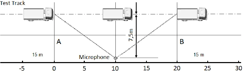
The test track for all vehicle categories is the same, a 20 meter long track with at the tenth meter microphones at both sides. These microphones are located 7.5 meters from the middle of the track and at a height of 1.2 meters, shown in figure 1 ‘PBN Test Track’.

3

For the speed and accelerations of the vehicles during the test is a difference made between categories N1 and N2,3. For the acceleration test the N1 category, the Sprinter and Vito of

Mercedes-Benz, has to drive 50 km/h at line A and then fully accelerate in a fixed gear until the rear reaches line B. For the constant speed test the vehicle has to drive 50 km/h between line A and B. The N2 and

N3 categories, all Daimler Trucks, shall have a stable acceleration with a vehicle speed of 35 km/h

(+/-5 km/h) at the end of the track. The gear, which has to be fixed during the test, shall be choose in a way that the engine speed at line B is 70-74% for N2 and 85-89% for N3 of the engine speed

where the engine develops its maximum power. More detailed information can be found in EU-Law 540/2014 [1].

2.3 Main noise sources

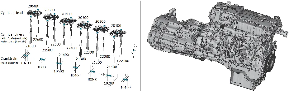
The noise of the vehicle comes from many different components and can be occurred by vibration of components or the direct vibration of air (tailpipe noise). The main noise sources, for the Mercedes Benz Actros on the PBN test, are from high to low: the engine, tire road interaction, rear axle, exhaust system, transmission, air intake system and drive shaft [3]. This ranking is however dependent on the design stage of the vehicle and the types of components used. An overview of models used for simulations of these sources is shown in figure 2.

Figure 2: Main noise sources of the Mercedes Benz ACTROS

2.4

PBN Simulations

Because of the new and lower limits, which reduce every four years, the prediction of the pass-by noise of new vehicles becomes more important than ever before. For this reason predicting the PBN of currently designed vehicles with acoustic simulation software is helpful to achieve the limits with design changes in an early stadium.

4

3.

Pass-by Noise Simulation Method

The virtual pass-by noise test requires a lot of sub simulations which use each other’s results. At first all the noise sources needs to be calculated individual with multibody and modal frequency response simulations to find the surface vibrations and the tailpipe noise. This results can be integrated in the exterior acoustic simulation. The separation of this simulations is necessary to reduce the size of the simulations and also to make it possible to share different results in multiple simulations. For example to use the same frequency response results of an engine model in different vehicle models. During developing the total simulation method there is attempt to integrated the results from different departments in order to reduce the amount of new models and simulations.

In this chapter the best method found to create the pass-by noise simulation of different vehicles is explained. It can be used as a manual to create models and simulations or to gain a better understanding of the working of the pass-by noise simulation program, explained in chapter 4. The sub-simulations are explained in the following order: multibody simulation for the engine with Matlab -> modal frequency response simulation in Nastran for an engine and exhaust -> the exterior acoustic simulation of the total pass-by noise in Actran.

3.1 Multibody Simulation - Matlab

The Multibody Simulation is the first step in the calculation of acoustic noise from the engine, exhaust and other noise sources. This MBS can be done with different simulation software and are mostly done by other departments of Daimler AG. For the engine programs as ADAMS are used to calculate the forces on specific points inside the engine. However, getting the right data for specific engines and engine speeds from other departments can sometimes take a long time.

Matlab program

To make first predictions of the acoustic behavior of the engine, the Matlab program create_loads.m is written to calculate the main forces by more simple formulas. This program is already written at earlier phase of the project [2]. However, the program is updated so it can calculate more engine situations, like four and six cylinder engines with different firing orders. Also the Matlab script is changed to make the integration with the PBN Program easier in a later stadium.

The program uses the gas pressures inside the cylinders as input for the dynamic load. This gas pressure results are provided by other departments in excel format. For every engine speed and position of the cylinder, from 0 to 720 degrees of the angle of the crankshaft, these pressures are listed.

5

Figure 3: Excitation node numbers for the six cylinder engine

The output of the program is modified to create a load case file in Nastran bdf format for every given engine speed. This load case file contains the DLOAD (Dynamic Load Combination) and RLOAD2 (Frequency Response Dynamic Excitation) cards in the same format as the MBS results from ADAMS are provided. This format is in more detail prescribed in 3.2.1.

Results of the MBS Matlab simulation appear to be inaccurate when compared to the ADAMS or GLW multibody results for the lower frequencies, shown in figure 4. Advised is to only use the Matlab program as first approximation when ADAMS or GLW data is not available yet.

6

3.2 Modal Frequency Response Analysis - Nastran

The modal frequency response analysis in Nastran can be done when the load cases at the nodes are defined for the FE models. The creation of detailed FE models is mostly done by other departments and is out of the scope of this report. Only the necessary modifications and the layout of the models and files to create the right input for the acoustic simulations are mentioned.

3.2.1 Engine

The required files for the Nastran simulation of the engine are the structure model, the radiation set and the load case if the ‘normal’ format is used. The structure model consists out of finite elements of the types: SPRING, MASS, RBE3 and 2, BAR, BEAM, TRIA3, QUAD4 and more. The elements for interest are RBE3 and 2, in which the MBS forces are introduced. For this reason the model should be check on the node numbers according to figure 3. The structure model also contains the material and geometry data for all different parts in bdf format.

The radiation set contains the numbers of the nodes for interest, which are the surface nodes to describe the shell noise in a later stadium. The radiation set needs to be created in a separated bdf file with the following format:

Radiation Set Structure bdf

SET 112 = 13000000 thru 13000028, 13000030, 13000031, 13000033 thru 13000042, 13000044 thru 13000051,

$ … NODE NUMBERS

The format is important for the PBN Program which will be described in chapter 4. The underlined code will be looked up by the program to check the files and to create the input file for the simulations. For the load case file, created with the MBS, the same applies. For every engine speed a separated load case file needs to be created in the following format:

Loadcase 800 RPM bdf

$DLOAD , SID, S, S1, P1, S2, P2, ETC...

DLOAD 300800 1.0 1.0 1001 1.0 1003 1.0 1005

1.0 1007 1.0 1009 1.0 1011 1.0 1013

. …

$ Sn = scale factor , Pn = RLOAD identification number

$ ID,DAREA ID, TABLE ID C(f), TABLE ID D(f)

RLOAD1 1001 1001 1001 1002

$ ID, Node Number, Component Number, Scale factor

DAREA 1001 10100 2 1.

$ ID

TABLED1 1001 $Freq, Phase Freq, Phase Freq, Phase

0.00-134. 15.83-317. 31.67 9.78 47.50 277. 63.33 146. 79.17-28.1 95.00 123. 110.83 189.

…

$ ID

TABLED1 1002 $Freq, Force Freq, Force Freq, Force

7

The RLOAD identification numbers can be split with commas or with spaces and the RLOAD1 and RLOAD2 formats are both allowed. The RLOAD is the frequency-dependent dynamic load of the form:

{𝑃(𝑓)} = {𝐴[𝐶(𝑓) + 𝑖𝐷(𝑓)]𝑒𝑖{𝜃−2𝜋𝑓𝜏}

The Nastran modal frequency response simulation can be created with an input fif file, in which all necessary data is provided and the models are assigned. The most important parts of this file are:

FIF file

SOL 111 $ select solution modal frequency response

CEND $ end Executive control statements

INCLUDE '/…' $ includes radiation set file

VELO(PLOT) = 112 $ export velocity for nodes in radiation set

ANALYSIS = MFREQ $ restrict output to modal frequency response analysis only

DLOAD = 30800 $ select dynamic load ID

FREQUENCY = 30000 $ select frequency range ID

BEGIN BULK

EIGRL 1500 -0.1 1600 $ extract eigenfrequencies for structural model

FREQ1 30000 17.5 17.5 72 $ select frequencies: ID, min, step, number

INCLUDE '/…' $ assigns: structure model and load case file

To select the frequency response simulation the code SOL 111 is used. The earlier mentioned DLOAD and models are included. With VELO the output data becomes the velocity of the radiation surface. These velocities will be the input data for the acoustic calculations.

The frequencies mentioned in the fif file corresponded with the engine speed of 2100 rpm of a four cylinder engine. The step size of these frequencies is determined by the 0.5 engine orders, in which the excitations are the highest [5], by the following formula: RPM/(60*4*0.5). A graph of the force in node 21200 is shown in figure 5a, in which the engine orders can be easily seen as the dark lines.

8

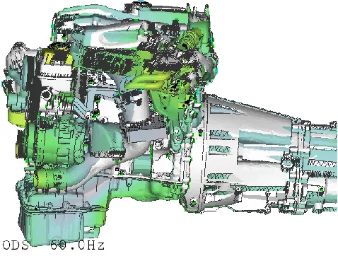
The results of the frequency response simulation of the surface velocities at 60 Hz are shown in figure 5b and are saved in an op2 result file. This file will later be used as input for the exterior acoustic calculation.

3.2.2 Exhaust

Simulating the exhaust requires a more complex fluid – structure interaction, which results in shell noise of the muffler and tailpipe noise at the end of the exhaust. Especially for trucks is the shell noise even important as the tailpipe noise [3]. The modal frequency simulation in Nastran requires two different models, the fluid model and the structure model of the muffler box. As input is an excitation on the exhaust given in the fluid domain, shown in figure 6, for all twelve ports (6-cylinder engine).

Figure 6: Fluid and structure model of the Exhaust

There are two output results desired, the shell and tailpipe noise, which are calculated in separated simulations. The simulation of the shell noise of the muffler box is comparable with the calculation of the engine, with as output the surface velocity on a radiation set, it only requires now the integration of the fluid model in the SOL 111 simulation. In this model the node numbers of the excitation ports needs to correspond with the node numbers in the load case file, in the format as explained in chapter 3.2.1 engine.

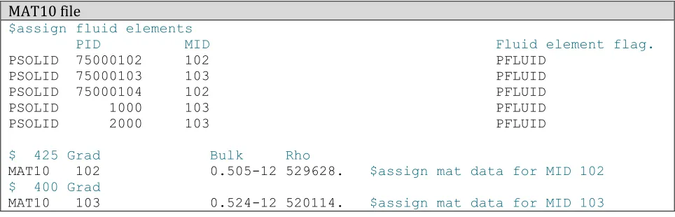
The fluid material data of an exhaust can differ over the tube, because of temperature difference. To take this difference in account a MAT10 material file is made. The material properties are assigned for every material ID (MID). The elements of the fluid also needs to be assigned as PFLUID elements, so Nastran will know the difference between the fluid and solid structure. A typical MAT10 file, which needs to be separated from the fif file for the PBN Program of chapter 4, looks like:

MAT10 file

$assign fluid elements

PID MID Fluid element flag.

PSOLID 75000102 102 PFLUID PSOLID 75000103 103 PFLUID PSOLID 75000104 102 PFLUID PSOLID 1000 103 PFLUID PSOLID 2000 103 PFLUID

$ 425 Grad Bulk Rho

MAT10 102 0.505-12 529628. $assign mat data for MID 102

$ 400 Grad

9

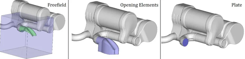
For the tailpipe noise a solution is created in order to find the particle velocities at this location. At the tailpipe a structure model is created, consisting out of a plate with a mass close to zero, over the complete cross section. This plate, shown in figure 7 in green, is supposed to behave in the same way as the particle velocity of the fluid without the plate. For this reason the plate has only one DOF in the longitudinal direction of the tailpipe and is assumed to be rigid. The bdf file of the plate is shown below, in which the SPC is the single point constrain to create the 1 DOF.

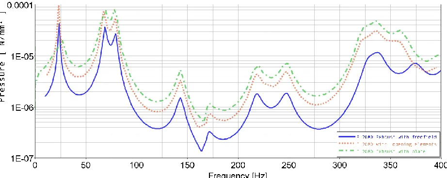
Because the tailpipe is a complex simulation, in which the acoustic behavior such as reflection of the acoustic wave is influenced by the ending, are different models tested. The first simulation is done with a free field, a large meshed fluid with absorbing elements at the boundary, around the tailpipe. The second with opening elements at the tailpipe, which mimic the free field. The last simulation is done with the light plate, for which it is possible to export the velocity at the nodes to the Actran model.

Figure 8: Three different simulations for the pressure at the tailpipe

The opening elements are normally used for exhaust calculations at Daimler. However, the results in figure 8 shows differences in the pressure value between the opening elements and free field. The pressure values at the plate are more close to the results with the opening elements. For all simulations are the eigenfrequencies very close to each other. More research is necessary to calculate the accuracy of the particle velocity mimicked by the plate. Also an research needs to be done to the differences between the free field and opening elements simulations.

Tailpipe Plate bdf

PSHELL 200 3001 1.0 3001 1.0 3001.8333333 0.0 -.5 .5

$Material data: Light Plate, density very low

MAT1 3001206010.079234.62 .3 .10E-09 .12E-4 0.0 0.0

GRID 1 1631.2302.6294-418.407 $Grid points

…

CTRIA3 100 200 118 121 111 $Elements

…

SPC 111 1 23456 $All nodes have one DOF, single point cons.

…

10

Figure 9: Pressure results at tailpipe for different scenarios

The simulations of the tailpipe and shell noise are both created with a input fif file, as also mentioned in 3.2.1 engine. To separate the simulations also two different input files need to be made, which will be done automatically by the PBN Program, mentioned in chapter 4. The most important parts of this file are:

FIF FILE

SOL 111 $ select solution modal frequency response

CEND $ end Executive control statements

INCLUDE '/…' $ includes radiation set file SHELL NOISE or

SET 750 = 1 THRU 200 $ includes radiation set TAILPIPE NOISE

SPC = 602 $ single point constrain set for tailpipe noise

VELO(PLOT) = 750 $ export velocity for nodes in radiation set

ANALYSIS = MFREQ $ restrict output to modal frequency response analysis only

DLOAD = 7502100 $ select dynamic load ID

FREQUENCY = 30000 $ select frequency range ID

BEGIN BULK

EIGRL 1500 -0.1 1600 $ extract eigenfrequencies for structural model

EIGRL 1501 -0.1 1600 $ extract eigenfrequencies for fluid model

FREQ1 30000 17.5 17.5 72 $ select frequencies: ID, min, step, number

SPCADD, 602, 1,75000001,75000002,111 $ combine multiple SPC's

INCLUDE '/…' $ assigns: fluid model, structure model or tailpipe plate,

material data and load case file

After the three simulations of the engine, muffler and tailpipe, the velocity results can be integrated in the exterior acoustic model.

11

3.3 Exterior Acoustic Simulation - Actran

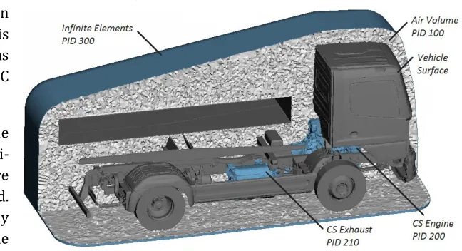
The last simulation step is the exterior acoustic simulation with Actran. For this simulation the radiation results of the engine and exhaust are needed from the Nastran simulation. Also models have to be made to describe the PBN simulation. The test track mentioned in 2.2 “Test procedure” can be translated to a virtual simulation track in Actran, in which the vehicle has a fixed position and the two microphones are replaced by a microphone array. For this reason only one simulation is required in which the complete PBN is calculated. However, effects of the vehicle speed, like air flow, are omitted. The virtual simulation is shown in figure 10 for a vehicle of five meters in length.

Figure 10: Virtual simulation track for the PBN

3.3.1 Actran models

Creating the FE models for the acoustic PBN simulations can be a time consuming job. The models need to describe the complete (reflection) surface of the vehicle and the radiation surfaces of the engine and exhaust. Because most vehicle models are available in detail, but without FE, a manual is written to extract the reflection surface for interest. This manual is included in appendix A: “Creating acoustic vehicle models from JT data”.

When the surface model of the vehicle is created the coupling surfaces of the engine and exhaust are required. This can be used to couple the results found on the BC mesh (radiation set) in Nastran with the input (coupling) surface in Actran. Creating the surfaces can be done by closing the holes in the BC model and wrap them in

ANSA or Actran. Important is that the coupling surface is as close as possible to the BC model.

The convex hull around the vehicle exists out of semi-infinite elements, which are used to describe the far field. This makes it possible to only use fluid elements inside the convex hull, which reduces the

12

hull and ground can be easily made and meshed in Actran. When all surface models are created and integrated in one file, the fluid volume can be meshed. It is important that the fluid mesh shares the same node numbers as the infinite and coupling elements at the boundaries. To create a standard for the PID’s, the following allocation is advised:

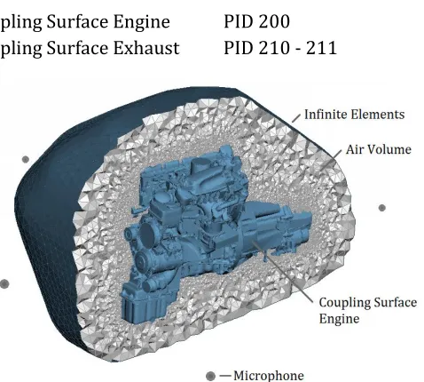
Air volume PID 100 Coupling Surface Engine PID 200 Infinite Elements PID 300 Coupling Surface Exhaust PID 210 - 211

3.3.2 Free Field Engine Simulations

The simulations in Actran are first tested with a free field simulation of the engine to get insights of the influence of different parameters. For these simulations the direct frequency response analysis is used. The model consists out of the coupling surface of the engine, an infinite element surface for far field and the air volume in between. Microphones are placed at every side of the engine at a distance of 1 m, shown in figure 13.

With the created model are many simulations done with small changes in the parameters. The parameters for mapping the results of Nastran on the couplings surface in Actran are the gap and planar tolerance in combination with the integration or sample method. The nodes of the Actran coupling surface must be in the “search volume” of the structure elements to map the surface velocity results from Nastran. This search volume is defined by

extruding the structure elements with a given gap tolerance and thereafter scaling the resulting volume by the planar tolerance, see figure 12. The gap tolerance is an absolute value, in meters or millimeters, while the planar tolerance is a relative value (0.1 = 10%).

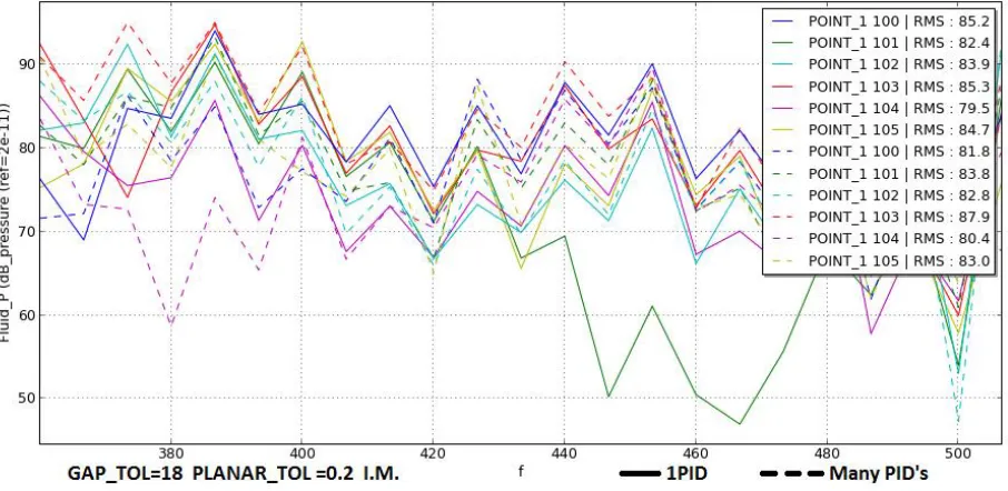
The sampling and integration method are two different methods to map the structure results on the acoustic mesh. With the sampling method is the structure mesh linear interpolated on the acoustic nodes, which is often a relative coarse mesh. This method could result in a loss of information, because some nodes of the fine structure surface are located too far away from the more coarse acoustic nodes. The integration method uses a conservative integration from the structure nodes to the acoustic mesh. With this method all information can be preserved if the acoustic mesh is in the reach of the search volume. For this reason the integration method is advised. However, during this project errors were found in the integration method of Actran 15.0 which led to inaccurate results, shown in figure 14 for a BC meshes with one and multiple PID’s. This PID’s should normally not give any influence in the acoustic results but it becomes clear that the influences are very large. These issues are solved for Actran 16.0 but not tested again. Advised is to use the integration method with

Figure 13: Free field simulation model in ACTRAN

13

multiple gap and planar tolerances and structure models (BC mesh) with only one or multiple PID’s to check if the results are stable. This could also be done for simulations with the exhausts structure and tailpipe noise.

Figure 14: Free field simulation results for structure models with one and with multiple PID's

3.3.3 PBN Simulations

When the right settings are found for the gap and planar tolerances (model dependent) and the results in free field simulations are expected to be accurate / stable for small changes, the PBN simulations can be done. To make the PBN simulation an edat file is created which contains all the input data. An example for the PBN simulation of a truck, with only the engine as load case, looks as follow:

EDAT FILE

BEGIN TOPOLOGY 1 BDF

FILE fluid_model_Truck.bdf $ integrate path to fluid model

BEGIN DOMAIN Air_Volume $ assign air volume with PID 100

PID 100

END DOMAIN Air_Volume

BEGIN DOMAIN Coupling_Surface_Engine $ assign CS of engine with PID 200

PID 200

END DOMAIN Coupling_Surface_Engine

BEGIN DOMAIN Infinite_Elements $ assign infinite elem. with PID 300

PID 300

END DOMAIN Infinite_Elements END TOPOLOGY 1

BEGIN TOLERANCE_LIST

BEGIN TOLERANCE 1 $ create tolerances

GAP_TOL 10 PLANE_TOL 0.1

14

In this model the microphone arrays, standard over 28 m, are integrated as fieldpoints and will have pressure and velocity results in the plt file. For the different load cases the following standard is made for the ID numbers: engine 50, exhaust structure noise 51 and tailpipe noise 75. These standards are important for the post processing in the developed PBN program in chapter 4. During this simulation perfect reflection is assumed for the vehicle and ground surface. It is advised to investigate the influence of this assumption with real reflecting values.

Simulations with a reduced air volume are tested to reduce the solving time. The reduction of the air volume lowers the number of nodes and elements. Because the microphones on the test track are located at a height of 1.2 m the influence of the vehicle surface above this height is expected to be small. A model of the van R2 is tested for this method, shown in figure 15 - 16.

BEGIN MATERIAL 1 $ create material (Air)

NAME Air FLUID

SOUND_SPEED { 340000, 0} FLUID_DENSITY { 1.225E-12, 0} END MATERIAL

BEGIN COUPLING_SURFACE 1 $ assign the CS of engine

NAME Coupling_Surface_Engine DOMAIN Coupling_Surface_Engine END COUPLING_SURFACE

BEGIN BC_MESH 1 $ integrate Boundary condition

Nastran_BDF Engine_BC_Mesh.bdf $ path to structure mesh

SURFACE 1

PROJECTION_TOL 1 $ gap and planar tolerance for mapping

BC_FILE Engine_2400LC_2100RPM.op2 $ path to Nastran op2 result file

BC_FORMAT Nastran_OP2

VELOCITY $ BC are surface velocities

END BC_MESH 1

BEGIN MULTIPLE_LOAD $ create multiple loads to simulate ..

BEGIN LOADCASE 50 $ engine (50), exhaust shell noise (51)

NAME Loadcase_engine $ and tailpipe noise (75) separately

{1,0} BC_MESH 1 END LOADCASE 50 END MULTIPLE_LOAD

BEGIN OUTPUT_FRF $ output setting

direct_2100RPM.plt $ create output file

BEGIN FIELD_POINT 1 $ create microphones at the track NAME Field_Points

58 $ number of microphones = 2*29=58

20000000 -11400 7500.0 365 $ right mic array series: 20000000

20000001 -10400 7500.0 365 …

30000028 16600 -7500.0 365 $ left mic array series: 30000000

15

Figure 15: Normal and reduced fluid model of the R2 Sprinter

The model is cut-off at a height of one meter, which results in a reduction of one million volume elements. Because the vehicle surface is connected to the semi-infinite elements, the vehicle surface will be extended in the same way it does with the ground surface. With a PBN simulation for a small frequency range the results are as follow:

Figure 16: PBN results of the normal and reduced fluid model of the R2 Sprinter

The dB values represents not the output which can be used to compare with real test data, because of the input date, however the comparison can be made the normal and reduced air volume model (RAV). It can be seen that the pressure values at the frequencies differ not a lot, at maximum 2 dB. For the overall sound pressure level (OSPL) the differences are less than 0.5 dB. The solving time was reduced by 25%. For these reason the reduction of air volume could be applied successfully at more accurate models.

Results

16

Figure 17: Truck results for engine and exhaust noise for 2100 RPM at 11 m

To gain more insight in the acoustic field around the vehicle model the visumaps (nff output of Actran) can be used. There are standard visumaps made for the PBN simulation, which are visual in figure 18 for the shell noise of the muffler box at 420 Hz. The visumaps contain two horizontal planes at 0 and -500 mm height, a vertical plane in the center of the model and to vertical planes along the microphone arrays.

17

4.

Pass-by Noise Simulation Program

The Pass By Noise program is created to make a standard method for all PBN simulations. This will save a lot of time, prevents faults during the process and makes all analysis structured in the same way. The program will lead the user through the complete process as mentioned in the earlier chapters. It is written for Python on Linux, which is free to use and pre-installed on the Linux blades inside Daimler. For installation the PBN_Program folder and the PBN_Program.py file needs to be copied. Starting the program in Linux can be done by typing “python PBN_Program.py” in Linux, which will give the start screen shown in figure 19. All coding of the programs and the structure of the folder can be found in the report “Pass By Noise Simulation, Coding of PBN Program” [4].

Figure 19: PBN Program Overview interface

The PBN Program exists out of four sub programs: New project, PBN Track, PBN Simulation and PBN Post. These programs can be used in the mentioned order to carry out the full PBN simulation.

4.1 New Project

First of all a new project can be created with the “New Project” program, shown in figure 20. Creating a new project for a specific vehicle type, means creating the standard folder structure used by all the PBN programs. By pressing open the user can import the path in which the new project will be created, with the folder name defined at Name. The second unfinished part of the program is the selection of the database location and type of vehicle. This part will be used in a later stadium to import automatically models and simulation results for specific configurations of vehicles. When everything is set, the create button can be pressed and the project folder with the five

18

The project folder will contain the following folders: 1_PBN_Track, 2_mbs, 3_nastran, 4_actran and results. The user can now copy or create all necessary models and files in the right folders according to figure 21. The use of the extensions for files (.bdf, .mat, …) and folders (_OP2, _BDF) are very important for the rest of the simulation, because the PBN programs searches on these formats, and should be done as shown in figure 21 in blue. Also when the content of the load case folder in 2_mbs or the BC (Boundary condition) folder in 3_nastran are created by the user, the files must be manually named to the corresponding engine speeds (…*RPM or …*rpm).

Figure 21: Structure and required files for the PBN simulation

4.2

PBN Track

The PBN Track program is the first simulation program which can be used after creating a new project. This program visualizes the exact engine and vehicle speed over the length of the track and calculates the engine speeds for the PBN simulations.

HOPE

19

PBN Track

The GUI of the PBN Track program is shown in figure 22a. At first the user can select the main project folder by loading a project. The GUI automatically updates and list all available MAT files found in the 1_PBN_Track folder of this specific project. Thereafter the user can choose the gear and the step size of the simulation.

This step size is necessary because for every engine speed there is a new simulation required in Nastran and Actran. The HOPE results contain unique engine speeds for every meter over the track, which would result in a very long simulation time in Nastran and Actran. The PBN Track program round these engine speeds for every meter to the selected step size (green line), shown in figure 22b. When the user is satisfied with the accuracy and number of simulations, the save button can be pressed.

Figure 22a: PBN Track Program b: Visualization of the engine and vehicle speed over the track

When the save button is pressed the PBN_Track.txt file will automatically be created, shown below. This text file includes a structured format of the engine speeds used and the microphones which corresponded to these engine speeds. It will be used by the PBN Simulation program and the post processor in a later stadium.

PBN TRACK FILE

#=================================================== # PBN Track file generated by theisma # PBN Track - Gear 3 - Stepsize 100 # Time: 2015-12-15 14:22:41 # Thomas Eisma - Daimler AG #===================================================

20 Microphones by 1900 RPM:

0 1 2 3 4 5 6 7 8 9 10 11 12 13 14

Microphones by 2000 RPM:

15 16 17 18 19 20 21 22 23 24

Microphones by 2100 RPM: 25 26 27 28

4.3 PBN Simulation Program

When all the models and files are created according to the earlier mentioned format, the main PBN Simulation Program can be started, shown in figure 23 and in large format in appendix B. This program is the coupling between all simulation programs mentioned in H3 and can carry out the simulation from MBS to modal frequency response analyses to the exterior acoustic simulation. All input files (.fif, .edat, …) for these simulations are created by the program itself, which saves the user a lot of time and prevents many errors.

Figure 23: The PBN Simulation Program Interface (large format: appendix B) PBN Simulation Program

21

in the format: minimum, maximum frequency. The step size for frequencies are dependent for of the corresponding engine speed. The program uses the 0.5 engine order as step size, which is calculated as: RPM/(60*4*0.5).

MBS-Matlab

If it is necessary to do the Multibody Simulation for the engine with the Matlab program mentioned in H3, the user interface under MBS- Matlab can be used. The Excel sheet with the gas pressures can be selected out of the list. Important is that the format of the Excel sheet is as follow:

 column A starting at row 4, the crank angles in degrees from 0 till 720.

 row 2 starting at column B, the engine speeds.

 row 3 starting at column B, the maximum gas pressures.

 starting at row 4 and column B, all the corresponding gas pressures in bar.

Besides this the number of cylinders (6 or 4), the firing order (starting with 1), and the mass and geometry of the cylinders must be filled in. As mentioned in H3, the results of the MBS – Matlab simulation are only accurate for the higher frequency range and can be used for a first approximation.

Nastran

The Nastran GUI makes it possible to select all necessary files needed for the modal frequency response analysis. The engine models can be selected in two different formats, the “normal” with only a bdf file of the structure model or the SEM format used by the Truck NVH department. For both formats a radiation set and a folder with load cases must be selected. The folder with load cases must contain a separate load case file for every engine speed used during the simulation, as shown in figure 21.

For the exhaust eight files can be selected to carry out the shell and tailpipe noise. All these files needs to be in bdf format and be created as explained in H3. The load case files for the shell and tailpipe noise are the same and must also be in the format as mentioned in figure 21.

If all models are selected there will be done three different Nastran simulations. By selecting only the engine models, only this calculation will be done in Nastran. Also for only simulating the shell noise of the muffler the tailpipe plate can be set on none, and for only simulating the tailpipe noise the structure model and radiation set of the exhaust can be set on none.

During simulation all necessary fif files will be created in the output folders. Thereafter the configuration file will be created and the jobs will be submitted to the calculation servers one by one. The fif files will not be deleted and can be used by the user in a later stadium and to store the simulation information.

Actran

22

The PID’s of the different elements in the fluid model can be filled in behind the option menu’s. It is recommended to us the standard pre filled values in order to create unity for all different models and vehicles. Below the option menus multiple parameters can be set:

 the mapping methods explained in chapter 3.3.2

 the front and ground coordinates of the vehicle model to calculate the microphone positions

 the material data for the air volume (fluid density and sound speed)

 the gap and planar tolerances used for mapping the structural results to the acoustic domain

 the interpolation order for the infinite elements

 the solver type: MUMPS or PARDISO. PARDISO is recommended for large models to reduce RAM usage.

Check and Start

An overview is given of the checks the program does when the Check button is used and the steps it takes when start is pressed:

Check if…

MBS: … gas pressure excel file exists

… output folder is unique … firing order start with 1

… firing order and number of cylinders match … all parameters are numbers

Nastran: … if all input files exists

… which simulations need to be done

… if BEGIN BULK is removed from bdf files

… which format is selected and if all required files are selected

… radiation set can be found and store the set ID for all rpms

… load case files can be found and store all DLOAD ID’s

Actran: … if all input files exists

… which simulations need to be done

… if OP2 files are available for all engine speeds … all parameters are numbers

When pressing the start button:

Start

Execute check (again)

Import current time, frequency domain and number of CPU’s

MBS: Write all user specified parameters to mbs_Matlab_input.txt

Change work directory to …/pbn_program/mbs/

Start create_loads.m in background (Matlab license necessary) Import parameters of mbs_Matlab_input.txt

Export load values to load case bdf file for every rpm Change work directory to specified output folder

Wait till simulation is done or stops after 1 minute

Nastran: Create simulation folder for every load case

Create fif file for every load case and engine speed

Import SET and DLOAD IDs, models, frequency… Change work directory to simulation folders

23

Actran: Import all user specified parameters

Create simulation path, named “hh:mm:ss + load cases”

If OP2 files come from “current Nastran Sim” check if finished

Create edat files for every engine speed based on settings

Change work directory to simulation path

Create configuration file and submit job

Wait till job is finished before sending next job (diff rpms)

Simulations finished or print errors

A more detailed description can be found in the coding in the report “Pass By Noise Simulation, Coding of PBN Program” [4].

4.4 PBN Post

When the complete PBN simulation is done, the PBN Post processor can be used to visualize the PBN in an easy way. The structure of the acoustic results created by the PBN simulation program is shown in figure 24. The results are organized per simulation and per engine speed. In these folders the direct.plt file can be found which contains the pressure and particle velocity results at the PBN microphones. Also NFF files are available when the visu map is selected. The PBN Post interface is shown in figure 25.

24

At first the project can be selected by with the open button. Thereafter the option menus for the different simulation results and PBN Track files are automatically updated and can be selected. Also the load cases (engine, exhaust, …) can be selected. The sum button will integrate a graph of the total PBN. The user can also select the option for colormaps, which will give a colormap in dB(a) for every load case.

When simulate is pressed, the program collects the results in the different engine speed result files (.plt) and couples these with the matching microphones, as written in PBN Trackfile. To create the colormaps the different frequency steps are interpolated on the frequencies of the first engine speed.

There are different ways to calculate the overall sound pressure level (OSPL) per microphone over the total frequency range. The formula Actran uses is a integration of the pressure levels over the frequency range:

𝑂𝑆𝑃𝐿𝑑𝐵 = 20 ∗ 𝑙𝑜𝑔10

√∫𝑓𝑚𝑎𝑥𝑃2 _𝑑𝑓 𝑓𝑚𝑖𝑛

𝑃𝑟𝑒𝑓

The formula PBN Post uses to calculate is a summation from the SPL of all frequencies:

𝑆𝑃𝐿𝑑𝐵(𝑓) = 20 ∗ 𝑙𝑜𝑔10

𝑃(𝑓) 𝑃𝑟𝑒𝑓

+𝐴𝑤𝑒𝑖𝑔ℎ𝑡𝑖𝑛𝑔

𝑂𝑆𝑃𝐿𝑑𝐵= ∑ 𝑃𝑟𝑒𝑓∗ 10^

𝑆𝑃𝐿𝑑𝐵(𝑓)

20

The difference in calculation can be explained as follow. In Nastran the modal frequency response analysis is done for the frequencies corresponding with the engine orders. This means that the inputs in Actran are mostly the highest excitations and not the average values. Integration of these results could give too high OSPL values. However, the summation is dependent of the number of samples and assumes that the results for other frequencies are relative low. It is advised to investigate these calculations in more detail to find the most accurate way.

Results

For the Atego truck the PBN simulation is done with as noise sources the engine and exhaust. The results of the PBN with an acceleration from 1900 RPM to 2100 RPM are shown by the post processor as figure 26. It creates a visual insight of all the different noise sources and the total dB(A) value. With selecting different combinations of the load cases and the summation, the effect of one load case can be seen on the total OSPL. The input data for these simulations are not accurate and therefor also not the dB(A) results shown in the figure. As soon as the correct input data is available the simulations can be execute easily again.

25

With colormaps selected in the GUI the PBN Post program will create a figure of every load case as shown in figure 27. With this function the dB level of every frequency can be seen separated. This create an insight in the dominated frequencies of the OSPL. Because the frequency steps of different engine speeds are not equal, the program interpolates all results on the frequency steps of the lowest engine speed.

Figure 27: PBN Results: Colormap Exhaust tailpipe noise at 2100 RPM

26

6.

Conclusion

A method for PBN simulations, with an engine and exhaust as noise sources, is developed. It includes a detailed explanation how the necessary models and simulations need to be set up. These simulations start with multibody simulations in which the main forces in an engine are calculated. With these results modal frequency response simulations can be made for the engine and exhaust in Nastran. The surface velocities of the engine and muffler are calculated together with the tailpipe noise as particle velocities. All noise sources are successfully integrated in an exterior acoustic simulation with the total vehicle model. This Actran simulation is done for the Atego truck of Daimler AG, with as result a visualization of the PBN of an acceleration test.

The explained way of solving the PBN simulation method is integrated in a new developed PBN program. This program makes it possible to create new projects with structured folders and shows an overview of how the user needs to provide the necessary input data, such as models and load cases. Thereafter the developed PBN simulation program makes it possible to couple MBS, Nastran and Actran simulations for different load cases and engine speeds. The program has a GUI which leads the user through all necessary steps and checks if the input data is correct. It saves time and prevents making input faults by creating all the necessary simulation input files itself, such as Nastran fif and Actran edat files. An included post processor makes it possible to visualize the PBN of different noise sources and the total PBN of different vehicles. The total program is flexible in the way that it can simulate different vehicles and can use different types of input data. The program can be used to improve the accuracy of PBN simulations, because it makes it possible to change separate input parameters or models. In the future more noise sources, such as the tires and intake system, can be add to the PBN program to complete the virtual simulation.

7.

Recommendation

With a new method for PBN simulations developed many new, uninvestigated research questions appear. Also, because the PBN program is not fully finished, it does not include all noise sources, recommendations can be made to improve the method and program.

 An improvement of the MBS in Matlab for engine’s

 The method in which a light plate is used to approximate the particle velocity of the tailpipe needs to be investigated on accuracy. This also counts for the differences in pressure of the meshed free field and openings elements at the tailpipe. An option can be integrating the internal fluid of the exhaust in the fluid model in Actran.

 The PBN simulation program needs to be include the intake system, experimental tire noise and the drive shaft / rear axle.

 The different formulas mentioned in chapter 4.4 for calculating the OSPL can be investigated on accuracy.

27

8.

Literature list

[1] REGULATION (EU) No 540/2014 OF THE EUROPEAN PARLIAMENT AND OF THE COUNCIL of 16 April 2014, “on the sound level of motor vehicles and of replacement silencing systems, and amending Directive 2007/46/EC and repealing Directive 70/157/EEC”, 27-5-2014

[2] Bachelorarbeit “Virtuelle Vorbeifahrtsimulation eines Nutzfahrzeug”, R. Halm, 03-09-2015

[3] Internal presentation Daimler AG, “VTA NVH CAE 2012“, D. Hackenbrioch, R. Visser, 2012

[4] Report, “Pass By Noise Simulation, Coding of PBN Program“, T. Eisma, 29-01-2016

28

Appendix A - Creating acoustic vehicle models from JT data

Creating good acoustic models for PBN simulations is an important and time consuming step. In order to reduce the creation time of proper acoustic meshes, a manual is written. The start point is the JT data of a vehicle. These contain the very detailed 3d models without surface or solid elements. An acoustic mesh only consists out of surface elements of the parts that have influence in the exterior acoustic behavior.

Teamcenter / NX

The JT data of the complete vehicle can be opened in Teamcenter. Because the vehicle models consist out of many parts, the best way to handle this is by showing only one subassembly at the time. From this subassembly all small and not interesting parts can be deselected / removed from the show. It’s very important to do this with a lot of attention, because the small parts are hard to mesh in a later stadium which takes a lot of time. These parts can be wires, tubes, bolts, springs and other small components. Also all parts which don’t have surfaces in the exterior fluid can be removed. The subassemblies can be exported as plmxml files. These files can be imported in NX in one assembly, where even more small parts can be deleted. Deleting parts is easier in NX, but NX handles large assemblies much slower than Teamcenter. Thereafter the model can be exported as STL file and opened in Ansa to create a bdf file. This bdf file can be used in Star CCM+ or Ansa to create a wrap of the model, shown in figure *.

Figure 28: STL and Acoustic mesh of the Sprinter R2 Ansa

In Ansa the model can be wrapped with the function NVH -> Ext. Acoustic -> Wrap -> Variable Length. For these important settings are a scale base length of 0 and a pre wrap treatment on the geometry instead of the mesh. This because the STL mesh is very different from a good acoustic mesh. Also a post wrap treatment is advised to create a better mesh. Disadvantages of Ansa are the small number of quality criteria and mesh parameters which can be set during wrapping. The mesh can be improved by using Mesh Tools -> Reconstruct, but this will not prevent intersecting of the elements anymore, which is by wrapping the case. Therefor the change is very large that new elements will intersect and a fluid mesh cannot be created. Intersecting elements must then be moved from each other by moving the nodes with Mesh -> Modules Buttons -> Grids -> Move. To prevent intersecting it is advised to remesh only small areas at the time. A (better) option is to wrap the model by the program Star CCM+.

Star CCM+

29

elements at the flat surfaces. Now the bdf file can be loaded in by File -> Import -> Import Surface Mesh. The surfaces (PID’s) can be found in Geometry -> Parts. Also the Curves of the model can be found here, but must first be calculated. This can be done right click on Curves -> Compute part curves and select the surfaces and options. The mark boundary perimeters for very large models can result in long waiting times. It is advised to select only Mark Sharp Edges, to better maintain the geometry during wrapping.

The next step is to create a new Mesh Continuum by right click on the continua folder. Thereafter right click on Mesh 1 gives the option to select meshing models. It is advised to select besides the surface wrapper also the surface remesher. The following options for the remesher and wrapper can be used:

Figure 29: Optional settings in StarCCM+

The base size of the mesh can be set on a convenient value of 100 mm, because most other settings are relative to this. Automatic Surface Repair is necessary to create proper elements, the quality can be set on 0.1 and the proximity on 0.01. Gap Closure is dependent of the model, but a too large value (+50 mm) will create too many closures in the final wrap. An important setting is the Surface (basic) Curvature, which default value is 36 pts/circle. At large two dimensional curved areas, for example the front bumper, this will result in a very small mesh. A better option for these areas is to set the surface curvature much lower. The surface Growth Rate can be set at a maximum of 1.2 to create a proper mesh.

The different regions can be assigned by creating a new region and thereafter new boundaries for every PID. For these boundaries the earlier mentioned quality options can be set individual. Also the earlier selected curves of the model can be added to a Feature Curve with individual mesh settings. A good option is create a separate PID for all the two dimensional curved areas, so the minimum mesh size can be set higher than the minimum mesh size at other areas. This can easily be done in Medina or Ansa by searching for elements which are connected with an maximum angle of 10 or 15 degrees. Also a separate PID for very detailed parts can be created, to set the target and minimum size relative low.

30

Figure 30: Different possible meshing’s of sheet metal

31

32

Appendix C

–

PBN Post Program results file

PBN TRACK FILE

#=================================================== # PBN Post file generated by theisma

# PBN Post - Loadcases: [1, 2, 3]

# PBN Track: PBNTrack_gear3_step100.txt # Time: 2016-01-27 10:30:04

# Thomas Eisma - Daimler AG

#===================================================

Values in dB(A) Loadcases: [LC Engine, LC Exhaust S, LC Exhaust T, ...]

Loadcase: Sum: