A graphical framework for representing the semantics of asymmetric
models
Paul E. Anderson Department of Statistics
University of Warwick Coventry, UK
CV4 7AL
Jim Q. Smith Department of Statistics
University of Warwick Coventry, UK
CV4 7AL [email protected]
Abstract
Bayesian networks (BNs) are useful for cod-ing conditional independence statements, es-pecially in discrete symmetric models. On the other hand, event trees (ETs) are conve-nient for representing asymmetric structure and how situations unfold. In this paper we report the development of a new graph-ical framework called the chain event graph (CEG). For symmetric models, all condi-tional independencies in a BN can be ex-pressed through the topology of a CEG. How-ever, unlike the BN, the CEG is equally ap-propriate for representing conditional inde-pendencies in asymmetric systems and does not need dependent variables to be specified in advance. As with the BN, it also provides a framework for learning relevant conditional probabilities. Furthermore, being a function of an ET, the CEG is a more flexible way of representing various causal hypotheses than the BN. This new framework is illustrated throughout by a biological regulatory net-work: the tryptophan metabolic pathway in the bacterium E. coli.
1
Introduction
Chain event graphs (CEGs) offer a way of combin-ing the advantages of event trees (ETs) and Bayesian networks (BNs). Like an event tree, the CEG can represent all possible events in asymmetric and sym-metric systems and describe how situations unfold. This is particularly pertinent for biological regulatory systems, where sequential processes such as activa-tion and repression need to be handled. However, unlike ETs, CEGs have the additional benefit that conditional independencies can be read off the graph directly from its mixture of directed and undirected
edges. The CEG has the same number of directed edges as the equivalent ET, but fewer vertices.
It has long been recognised (see e.g. [Geiger et al., 1996]) that although BNs are very expressive of certain types of conditional independence statements through theorems like d-separation, they are poor at expressing asymmetric structure. Analogues of the d-separation theorem can be derived for CEGs. Indeed, for sym-metric problems, it can be shown that all statements passing the d-separation criteria can be read from the topology of the CEG. But implied conditional inde-pendence can be read from the graph of the CEG for highly asymmetric models as well, when the corre-sponding BN can be complete and so totally uninfor-mative.
Further, if a model description is based on sequences of occurrences, it is often difficult to choose an appro-priate set of functions of measurement random vari-ables that will exhibit useful conditional independen-cies. Inspection of the topology of the CEG immedi-ately guides the construction of these collections of functions, as illustrated in section 3.2. In BNs of course, it is assumed that such random variables are given, so this issue is never addressed.
Because the CEG encodes conditional independence structure, making certain collections of its vertices ex-changeable, it is straightforward to estimate, see sec-tion 4. In particular, using an analogue of local and global independence and complete random sampling (so that the likelihoods separate), conditional proba-bilities in the graph can be estimated in a conjugate way.
expressed succinctly. Furthermore, as demonstrated below, results such as the backdoor theorem [Pearl, 2000], which deduces the identifiability of a cause in a partially observed system through examination of the topology of a BN, also have their analogues in CEGs: see section 5.
In the next section, we shall describe a biological sys-tem — the regulation of an important amino acid, tryptophan, in bacteria — and use it to illustrate the definition and construction of an ET and then a CEG. Later, we consider the elicitation of conditional inde-pendence statements, estimation from real data and explore manipulation and causation within this model.
2
The ET for Tryptophan Regulation
The CEG is useful for expressing models that are most naturally described in terms of processes rather than cross-sectional interdependencies. Biological regula-tory mechanisms are one domain where this feature may be exploited. We shall now detail a running ex-ample of such a process.
In humans, tryptophan is one of the nine essential amino acids that are required for normal growth and development, but it cannot be produced endogenously. The bacterium Escherichia coli, commonly found in the human colon, also needs a supply of tryptophan to survive, but has the ability to synthesise its own if starved. Further, if tryptophan becomes plentiful in the local environment, then its production can be switched off. As with many biological systems, the underlying mechanisms are complicated, act at differ-ent timescales and depend on several contingencies. However, with some simplifying assumptions, we can describe this system in terms of the probabilities of cer-tain events occurring. (See [Ito and Crawford, 1965] for one of the original descriptions of tryptophan regu-lation in the biological literature and [Somerville, 1992] for a recent review.) For simplicity, we have focused on two regulatory mechanisms: feedback enzyme inhi-bition andgene repression.
When a bacterium receives an increased level of tryp-tophan, the first process that acts is chemical: feed-back enzyme inhibition, FEI. Essentially, there are a series of enzymes that catalyse successive steps in a metabolic pathway culminating in the production of tryptophan. However tryptophan, the end-product of this pathway, inhibits the first enzyme. Thus if tryp-tophan is plentiful, there is a greater chance that the first enzyme is inhibited, cutting the chain of enzyme catalysis and resulting in a decrease in the production of tryptophan. Similarly, if the level of tryptophan is reduced, then there is a smaller chance that the first enzyme is inhibited, so tryptophan production can
in-crease. FEI takes place immediately in response to a change in exogenous tryptophan levels.
High temp Tenv↑
FEI√ GR√
SG EG BG
GR×
SG EG BG
FEI×
GR√
SG EG BG
GR×
SG EG BG
Tenv↓
FEI√
SG G
FEI×
GR√
SG G
GR×
SG G
Low temp Tenv↑
FEI√ GR√
SG EG BG
GR×
SG EG BG
FEI×
GR√
SG EG BG
GR×
SG EG BG
Tenv↓
FEI√
SG G
FEI×
GR√
SG G
GR×
[image:2.595.327.554.115.534.2]SG G
Figure 1: Full event tree for tryptophan regulation in E. coli. Vertices shaded in the same direction belong to the same stage and position. The two filled vertices are in the same stage, but different positions. Edge labels are explained in the text.
available to bind to and activate TrpR, relieving re-pression and allowing exre-pression of the trpgenes, and hence increasing tryptophan production.
The ET of this simplified version of the tryptophan regulation model is shown in figure 1 and constructed below. Recall that an event tree,T, consists of a set of vertices V(T) and a set of edgesE(T) with one root vertex,w0. The members of the set of non-leaf vertices
(i.e. those vertices that do not terminate a branch),
S(T)⊂V(T), are calledsituations. Every situation is a precursor of future developments, so each situation
v ∈ S((T)) has an associated random variable X(v) whose event space labels the edges (v, v0) emanating from v.
In building the ET, both verbal descriptions [Campbell and Reece, 2002] and mathematical models [Santill´an and Mackey, 2001] guided us before consultation with a microbiology expert.
Imagine a population of E. coli grown in a minimal medium in a chemostat. That is, they are supplied with the bare essentials needed to survive. Our model describes the events that affect a bacterium. Differ-ent bacteria may follow differDiffer-ent root to leaf paths. The chemostat can be kept at two temperatures: high and low. The potential subsequent events will not be affected by this condition, but the probabilities that certain molecules bind and stay bound will differ, as will the growth rate and tryptophan requirements of the bacterium. Therefore the branches from these two situations will look the same, although the probabili-ties on the edges will vary.
An experimenter can use the chemostat to manipu-late the level of environmental tryptophan up, repre-sented by the event Tenv↑, or down, Tenv↓. After this
change, we want to see how the bacterium responds. Under the first response, FEI either takes place, FEI√, resulting in a drop in the amount of tryptophan pro-duced, or not, FEI×, leading to a rise. Over a longer period, GR will either occur, GR√, meaning less tryp-tophan is manufactured, or not, GR×, so that more is made. Depending on the events that have already taken place, the growth state will be different. We permit four possibilities:
• SG: synthesised tryptophan is the main
contrib-utor to growth.
• EG: environmental tryptophan is the main
con-tributor to growth.
• BG: synthesised and environmental tryptophan
contribute equally to growth.
• G: the bacterium does not grow.
Contingent on previous events, these states can be seen as efficient (for example,SGif there is little tryptophan
in the environment) or inefficient (SG if tryptophan
is abundant). Of course, in reality there would be a spectrum of intermediate events at all levels of the ET. These could be included by adding more edges. As our example is intended to be illustrative rather than comprehensive, for visual clarity we have limited the number of possibilities.
The unfolding of these processes can be read from the tree. For example, when starving the E. coli of tryptophan, no external supply is available, so we can simply exclude the edges for EG and BG in this case.
When tryptophan is plentiful, the bacterium will al-ways grow, soG cannot occur. If there is tryptophan starvation and FEI takes place, then there is so little tryptophan that it is very likely that the bacterium will not grow, leading straight to the choice of final states.
The point to notice here is that a BN could never fully express the qualitative structure of the events graphically, and the more complicated the regulatory model the more that is lost. On the other hand, we demonstrate below that the CEG — a function of the ET along with collections of exchangeability state-ments — can often represent all the elicited qualitative structure; sometimes fully. Therefore, within these contexts, the CEG provides a much more expressive framework than the BN for interrogating the model’s implicit conditional independencies, and embellishing an unmanipulated model with causal structure. It captures conditional independence statements through making the assertion that certain random variables at particular collections of situationsX(v) are identically distributed.
Note that since its edges represent dependency, events with zero probability cannot be represented in a BN. However, being derived from an ET, these can be in-corporated in the CEG by simply not including the relevant edge. As illustrated by our example, in many problem descriptions elicited using a tree, the length of root to leaf paths associated with various sequences of situations are often different. Whilst this is han-dled naturally in the CEG, this type of structure can only be represented in a BN by artificially adding more deterministic relationships to the system.
3
The Chain Event Graph
3.1 Definitions
demon-strated later in the running example, some situations
v ∈S(T) will have random variablesX(v) with iden-tical distributions to other situations. Thus there is often a partition {u : u ∈ L(T)} of S(T) associated with an elicited ET such that for v, v0
∈ u, the dis-tribution of X(v) is the same as the distribution of
X(v0
). Henceforth, the elements of L(T) are called stages. Note that as far as their distributions are con-cerned,X(v) could also be indexed by their stagesu.
In figure 1, each situation is in a different stage except for the vertices shaded in the same direction and the two solid vertices. In these cases we expect biologically that the probability of the next event is represented by the same random variable, hence they are in the same stage. Extending the idea of a stage, two situations
v, v0
are said to be in the samepositionif their futures, described by the subtrees T(v),T(v0
) with rootsv, v0
, are such that T(v) and T(v0
) are topologically iden-tical and all pairs of situations at equivalent locations in the subtrees are in the same stage.
In our example, the shaded vertices are in the same position since the leaves v, v0 are terminal situations:
T(v) andT(v0) contain no other situations other than
v and v0. The solid situations are not in the same
position however, since whilst the topology of their associated subtrees is the same, their corresponding situations are not in the same stage.
The CEG collapses all vertices at the same position into a single vertex and then joins positions at the same stage by an undirected edge. This allows condi-tional independence statements to be read with ease. In addition, all leaves of the tree are joined to a single sink vertex, w∞. This step highlights the paths (not
the leaves) as the atoms of event space.
We note that the set of positions {w : w ∈ K(T)}
partitionS(T) and thatK(T) is at least as refined as
L(T). For typical large scale biological applications, the partitions K(T) and L(T) have an organisation that can be subsequently exploited to derive deduced conditional independence. Our simplified illustrative example has, however, been chosen to exhibit a mini-mum of such structure.
Formally, the CEGC(T) is defined as the mixed graph whose vertex set is V(C(T)) = L(T)∪ {w∞}, whose
directed edges are Ed(C(T)) =E1(C)∪E2(C) where
E1(C) = {(w(v), w(v0)) : ∃v[1] ∈ w(v), v[2] ∈ w(v0)}
and E2(C) = {(w(v), w∞) : ∃v[1] ∈ w(v), v[2] ∈
V(T)\S(T)}with (v[1], v[2])∈E(T), and whose undi-rected edges Eu(C(T)) = {(w, w0) : u(w) = u(w0)}
withw6=w0
∈V(C(T)).
The CEG contains all the information of the ET since its root to sink paths are in a one-to-one
correspon-w0
1 2
4 16
99
17
5 10
18
19 High temp
Tenv↑
Tenv↓
w∞
BG EG SG
BG EG SG
3 6
20
99
21
7 14
22
23 Low temp
Tenv↑
Tenv↓
SG
G SG
[image:4.595.330.555.70.298.2]G
Figure 2: Chain event graph skeleton for tryptophan regulation inE. coli. Edge labels are explained in the text and the nodes are numbered consistently with fig-ure 3. w0 is the root node, w∞ the leaf vertex. Only
some terminal edges are labelled for clarity. Note the undirected edge joining the high and low temperature nodes. The dots denote subsequent events not shown here. Figure 3 shows part of this CEG in detail, from the high temperature node onwards, with all edges la-belled.
dence with the root to sink paths of its ET. On the other hand, all the stages and positions can be read from its topology. This gives a graphical depiction of conditional independence implicit from the model description akin to the BN. In [Smith, 2004] it is proved that, unlike probability graphs [Bryant, 1986] and probability decision graphs [Jaegar, 2004], in the special case when a qualitative model can be fully de-scribed by a finite discrete BN, it can also be fully described by a CEG. Thus for discrete problems, the CEG is a genuine generalisation of the BN. It also gen-eralises the discrete MDAG [Thiesson et al., 1999].
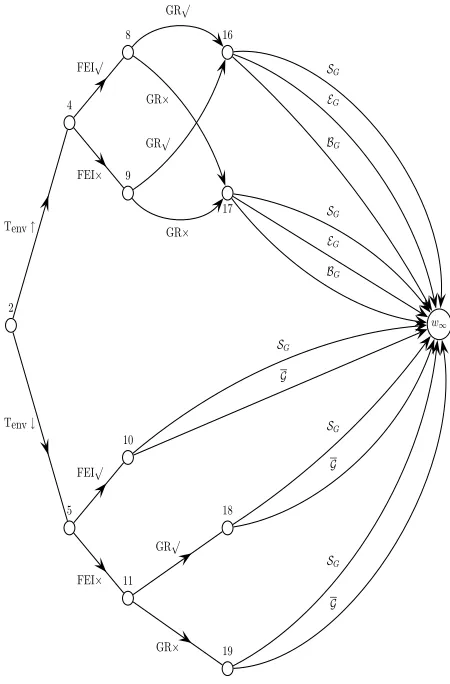
With the CEG defined, we can now draw the CEG for our example. So that all the features can be seen, figure 2 gives a skeleton outlining the start and end of the CEG, whilst figure 3 shows a part of the CEG in close-up. Firstly, we join all the leaves of the tree to one sink vertex, w∞. Having elicited the stages
2 4
8 16
9
17
Tenv↑
FEI√
FEI×
GR√
GR× GR√ GR×
w∞
BG
EG
SG
BG
EG
SG
5 10
11
18
19 Tenv↓
FEI√
FEI×
GR√
GR×
SG
G
SG
G
SG
[image:5.595.75.300.74.416.2]G
Figure 3: Part of the chain event graph for tryptophan regulation inE. coliassociated with high temperature. The topology is repeated for low temperature. Edge labels are explained in the text. See figure 2 for the overall structure.
3.2 Conditional Independence in a CEG
As with the BN, various conditional independence statements implied from an elicited CEG can be read directly from the topology of its graph. In this pa-per we restrict ourselves to the discussion of one result linking the topology of the graph to conditional inde-pendence statements: many others are given in [Smith, 2004]. First, we need two concepts. We call a collec-tion of posicollec-tions, Ω, afine cut if all paths fromw0 to
w∞ have to pass through exactly one member of Ω.
For the tryptophan regulation example, the set of ver-tices Ωeg ={3,10,11,16,17}shown in figures 2 and 3
constitute a particular fine cut. Aseparator Q(Ω) is a random variable taking different values qi for each of
the paths in the path event space that pass through a different elementωi of the cut Ω.
LetZ(Ω) denote a random variable whose atoms have an event space that corresponds to the paths ofCthat
start at the root vertex and end at a position ω∈Ω. Informally, Z(Ω) documents events that happen up-stream of Ω. Let X(Ω) denote a random variable whose atoms have an event space that corresponds to the paths ofC starting at an element ω∈Ω and end-ing at ω∞. ThusX(Ω) describes events that happen
downstream of Ω. It is easy to prove [Smith, 2004] that
X(Ω)aZ(Ω)|Q(Ω) (1)
The meanings of all the variables can be deduced from the topology ofC and, unlike for the BN, do not nec-essarily just concern disjoint subsets of a given set of random variables, but can be functions of these.
To illustrate equation (1), consider again the cut Ωeg
defined above. Assume you learn the values of a function Q(Ωeg). The value of the variable Z(Ωeg)
gives additional information about whether a sequence passed through situation 8 or 9. Note that this is not learned from Q(Ωeg). The random variable X(Ωeg)
reveals the unfolding of events after observing a low temperature, and also whether or not GR occurred af-ter observing a high temperature, Tenv ↓and FEI×.
Equation (1) tells us that whether an observation passes through 8 or 9 is irrelevant to predictions about
X(Ωeg) once we learn the value of Q(Ωeg).
Note that this conditional independence statement does not simply concern the original variables Tenv,
etc, but functions of them. It is not always possible to read this type of implication from a BN on the orig-inal variables. As with the BN, suitably interpreted subsets of these implications, read directly from the graph, can be fed back to the expert for validation.
4
Estimation of CEGs From Data
We now move to the problem of estimating probabili-ties on a CEG, C, from data. Note that the probabil-ities needed to fully specify C are the densities p(πu)
of the primitive probabilities {πu ∈ Πu : u ∈ L(C)}.
These correspond to the random variables{X(v) :v∈
The CEG shares an analogous property and hence in-herits these capabilities. To appreciate this, it is use-ful to visualise a network of simulators on an event tree which represent the data generating process: one for each position. Imagine a computer experiment in which random, independent draws are made from sim-ulators lying along a path in C starting at the root vertex,w0. As with BNs, nothing is lost if we assume
that the CEG is generated in this way [Riccomagno and Smith, 2005].
Now assume that the vectors of primitive probabilities
{p(πu) : πu ∈ Πu}are all independent of each other.
When we have a complete sample of n observations, we samplenroot to sink paths {λi: 1≤i≤n}: each
λibeing an instantiation of the underlying event space
XofC. In the simulator world, observing a root to sink pathλof lengthN(λ) just corresponds to a sequence of independent realisations of theN(λ) random variables
X(v) lying along that path. So, given {πu ∈ Πu :
u ∈ L(C)}, the probability of λ occurring is simply the product of the probabilities πu on this path: a
monomial in{πu∈Πu:u∈L(C)}. Since we observen
such paths independently, it is therefore easy to check that the likelihood of this sample can be written
L(π|λ1, . . . , λn) = Y u∈L(T)
nY(u)
i=1
πi(u)ri(u)
where ri(u) is the number of times the ithedge from
a position v ∈ u is traversed in the observed paths
{λ1, . . . , λn}. The vectorπ has as components all the
primitive probabilities andn(u) is the size of the state space ofX(u).
The product form of this likelihood means that if
{p(πu) : πu ∈ Πu}are all a priori independent — so
that their densities also respect the same product form — then Bayes’ theorem ensures that the product form is respected a posteriori. That is, the vectors of prim-itives are a posteriori independent. Further, suppose that for eachu∈L(C), p(πu) is a priori independently
Dirichlet distributed α = (α1, α2, .., αn(u)), D(α(u)),
so that its density is given by
p(πu) =
Γ(Pni=1(u)αi(u)) nQ(u)
i=1
Γ(αi(u)) n(u)
Y
i=1
πi(u)αi(u)
−1
Then Bayes’ theorem also allows us to show that each of these densities is Dirichlet a posteriori.
To illustrate this, suppose we observe two paths (λ1, λ2) associated with independent replicates of the
process where: λ1 = {High temp, Tenv ↑, FEI√,
GR√, EG} and λ2 = {High temp, Tenv ↑, FEI×,
GR√, EG}. It follows that the likelihood is given
by π1:22 π22:4π4:8π4:9π8:16π9:16π216:EG, where πa:b is the
probability that the next situation is vertex b given that the current situation is a. So, for example, the posterior distribution of the situation 2 is given by
D(α∗(2)) whereα∗
1(2) =α1(2) + 2 andα∗2(2) =α2(2),
whilst for situation 16 we have α∗
1(16) = α1(16),
α∗
2(16) = α2(16) + 2 and α∗3(16) = α3(16). Thus,
prior to posterior conjugacy is not unique to discrete BNs. It is also a property under ancestral sampling of the more general class of CEGs, see [Riccomagno and Smith, 2005] for more details.
In applications like the tryptophan pathway, we have two complications. First, the sample countsri(u) may
not be available without measurement error and may be dependent. Second, observations of many of the sit-uations may be hidden. For example, microarray anal-ysis and polymerase chain reaction (PCR) experiments may be able to tell us the rate of gene transcription (and thus we may be able to infer whether gene repres-sion has occurred), and other techniques can measure enzyme activity. However, this data may not always be available or accurate. Such problems mean that con-jugacy (and sometimes identifiability) is lost. We then need to resort to approximate methods (e.g. [Cowell et al., 1999]) that retain the algebraic product form or use more time consuming numerical algorithms. But exactly the same issues are faced when modelling with BNs. Hence, these issues are intrinsic to missing data problems in general: they are not an artifact of the CEG.
5
Causal Structures and CEGs
5.1 The Causal CEG
Shafer [1996] cogently argues that definitions associ-ated with causality are much more generally expressed in terms of an ET than a BN. Lying between the ET and the BN, the CEG retains many of the expressive advantages of the ET. However, the richness of its topology permits the development of strictly graphi-cal criteria to resolve issues such as whether or not an effect of a manipulation is identifiable in the light of a partially observed system — assuming the CEG is causal. Here we outline how to construct causal CEGs and state an analogue of Pearl’s backdoor criterion ap-plicable to such causal CEGs.
turn off the simulator associated with X and set it to
b
x with probability one, and to rewire all simulators in the system that take x as an input and set this in-put to the value xb, before running the network. This appears the obvious definition for the causal effect of manipulating the value ofX to bx.
This analogy extends to the CEG in a very natu-ral way. Recall that each position w has a simula-tor, or random variable, X(w) associated with it. A positioned manipulation of the position w simply re-places any random variable X(w), labelled by its po-sition w, by its manipulated value xb(w) with proba-bility one. bx(w) is then used as an input for a sub-sequent simulator. Non-atomic positioned manipula-tion {X(w) = bx(w) : w ∈ W} of a set of positions simply performs this substitution for all w ∈W. For example, we may decide to concentrate on how the bacterium responds at high temperatures only. In this case, we set X(w0) = High temp. The result of this
(causal) manipulation on the distribution of a second random variableY can now be calculated by making the appropriate substitution into the factorisation of the elementary path events.
Shafer [1996] rightly points out that not all causal hy-potheses need to be thought of in terms of manipula-tions and not all causal manipulamanipula-tions are necessarily positioned. However, in many situations we meet in practice, we want to consider positioned manipulations and certainly many authors [Pearl, 2000, Spirtes et al., 1993] restrict their attention to subsets of these types of manipulations. Note that manipulations of this type (gene, cell, environmental) are common in experiments on regulatory networks [Schimd et al., 2004]. A full discussion of such issues is given in [Riccomagno and Smith, 2005].
It is easily checked that the atomic manipulation of a BN corresponds to the special case of setting to xb, say, all the values of the variablesX(w) along special classes of fine cutW. Note that this cut will define an event space for which the manipulated random vari-ableX is measurable.
5.2 The Backdoor Theorem
We end the paper by demonstrating how the topology of a CEG can be used to answer questions about the identifiability of a cause. The topology of the BN has of course been used for such purposes, see [Pearl, 2000].
If M is a random vector, whose sample space is a
subspace ofX, then for each valuemofM, let Λ(m)
denote the set of paths λ(m)∈X that are consistent
with the event{M =m}.
Our result concerns three fine cuts in a CEGC
Ωa = {w:w=wj(a,λ)for someλ∈X}
Ωb = {w:w=wj(b,λ)for some λ∈X}
Ωc = {w:w=wj(c,λ)for some λ∈X}
where j(a, λ) denotes the (integer) distance from w0
to a position in Ωa on a root to sink pathλ. For each
λofX, we now specify that
j(a, λ)< j(b, λ)≤j(c, λ)
In this sense it can be asserted that the fine cut Ωa lies
before Ωbwhich in turn lies before Ωc. Let the fine cut
Ωb(−)={w:w=wj(b(−),λ)for someλ∈X}
be the set of all positions that are a parent of a position Ωb in C. Clearly,
j(a, λ)≤j(b(−), λ)< j(b, λ)≤j(c, λ)
To find a CEG analogue of Pearl’s backdoor theorem (BDT) we need to find a graphical property of a CEG that ensures that a random variable M = (Z, X, Y)
identifies the total cause (redefined for the extended environments defined by the CEG). The random vari-ablesX and Y are given and an appropriate random variable Z can be constructed from the topology ofC
using the BDT. SupposeZis measurable with respect to Ωa and X is measurable with respect to Ωb. For
the BDT, attention is restricted to the case where Z
happens beforeX andY.
For a CEG, this means that Z can be expressed as a coarsening Ωz (whose intersecting paths are {Λ(z) :
z ∈ Ωz}) of a fine cut Ωa “before” the fine cut Ωb,
in the sense defined above. A cut Ωc, as used in the
theorem below, separates the events {Y = y} from
{Z =z, X=x}in the sense that all paths consistent with {Z =z, X =x, Y =y}pass through a position
c(z, x) ∈Ωc. That is, c depends on z and x but not
y. Finally, let B(−, z, x) be the set of all positions
b∈Ωb(−) consistent with the event{Z=x, X=x}.
It is now possible to search for appropriate fine cuts Ωa and Ωc with reference to a given fine cut Ωb, with
a topological property given in the theorem below. In this way, we can find an appropriate random variable
Z such that (Z, X, Y) identifies a given total cause.
TheoremIf for any given valuez∈Ωz ofZ either:
1. all root to sink paths inCin Λ(z, x) pass through a single positionc(z, x),or
then the total cause, p(y||x), on y ∈ Ωy for a given
x∈Ωx is identified from (x, Y, Z) and is given by the
equation
p(y||x) = X
z∈Ωz
p(z)p(y|z, x)
where
p(z) = X
λ∈Λ(z)
π(λ)
p(y|z, x) = X
λb∈Λ(z,x,y)
π(λb)
andp(y||x) denotes the probability thatyoccurs given that X has been manipulated tox[Lauritzen, 2001].
See [Riccomagno and Smith, 2005] for the proof of this result. Note that unlike the BDT for the BN, the con-ditioning random variable (vector) Z need not be a subset of the measured vector of variables but can be any function of preceding measurements. Also, con-dition one or two of the theorem may be invoked de-pending on the value ofz∈Ωz.
6
Discussion
The chain event graph is a powerful graphical con-struction for asymmetric and symmetric models that can be used to answer inferential questions in anal-ogous ways to the Bayesian network. The Markov theory for the CEG, whilst not yet complete, is well developed. The challenge now is to demonstrate the efficacy of this class of graphical models in real large scale applications.
Acknowledgements
We are very grateful to Dave Whitworth for providing expert knowledge and helping us to clarify and improve the event tree and CEG for the tryptophan pathway. Paul E. Anderson is funded by EPSRC and BBSRC as part of the Interdisciplinary Program for Cellular Regulation (IPCR) and the EU TMR network BioSim.
References
R. E. Bryant. Graph-based algorithms for Boolean function manipulation.IEEE Transactions on Com-puters, 35(8):677–691, 1986.
N. A. Campbell and J. B. Reece. Biology. Addison Wesley Student Series. Benjamin Cummings, 6th edition, 2002.
R. G. Cowell, A. P. Dawid, S. L. Laurtizen, and D. J. Spiegelhalter. Probabilistic Networks and Expert Systems. Springer-Verlag, 1999.
D. Geiger, D. Heckerman, and C. Meek. Asymptotic model selection for directed networks with hidden variables. InProceedings of the 12th Annual Confer-ence on Uncertainty in Artificial IntelligConfer-ence (UAI-96), pages 283–290, Portland, OR, 1996. Morgan Kaufmann Publishers.
J. Ito and I. P. Crawford. Regulation of the Enzymes of the Tryptophan Pathway inEscherichia Coli. Ge-netics, 52:1303–1316, 1965.
M. Jaegar. Probabilistic decision graphs — combin-ing verification and AI techniques for probabilis-tic inference. Int. J. of Uncertainty, Fuzziness and Knowledge-based Systems, 12:19–42, 2004.
S. L. Lauritzen. Causal inference from graphical mod-els. In O. E. Barndorff-Nielsen, D. R. Cox, and C. Kluppelberg, editors, Complex Stochastic Sys-tems, pages 63–108. London: Chapman and Hall, 2001.
J. Pearl. Causality, models, reasoning and inference. Cambridge University Press, 2000.
E. Riccomagno and J. Q. Smith. Chain Event Graphs to Represent Bayesian Causal Hypotheses. Submit-ted to J. Royal Statist. Soc. B, 2005.
M. Santill´an and M. C. Mackey. Dynamic regulation of the tryptophan operon: A modeling study and comparison with experimental data. PNAS, 98(4): 1364–1369, 2001.
J. W. Schimd, K. Mauch, M. Reuss, E. D. Gilles, and A. Kremling. Metabolic design based on a coupled gene expression — metabolic network model of tryp-tophan production in Escherichia coli. Metabolic Engineering, 6:364–377, 2004.
G. Shafer. The Art of Causal Conjecture. Cambridge, MA, MIT Press, 1996.
J. Q. Smith. Conditional independence and chain event graphs. Submitted to Artificial Intelligence, 2004.
R. Somerville. The trp repressor, a ligand-activated regulatory protein. Prog. Nucleic Acids Res. Mol. Biol., 42:1–38, 1992.
D. J. Spiegelhalter, A. P. Dawid, S. L. Lauritzen, and R. G. Cowell. Bayesian analysis in expert sys-tems (with discussion).Statistical Science, 8:219–83, 1993.
P. Spirtes, C. Glymour, and R. Scheines. Causation, Prediction, and Search. Springer-Verlag, New York, 1993.