The effect of global financial crisis on trade elasticities: Evidence from BRIICS countries and Turkey

Munich Personal RePEc Archive

The effect of global financial crisis on

trade elasticities: Evidence from BRIICS

countries and Turkey.

Ketenci, Natalya

2013

The effect of global financial crisis on trade elasticities:

Evidence from BRIICS countries and Turkey.

Natalya Ketenci1

(Yeditepe University, Istanbul)

Abstract

The effect of the global financial crisis on the international trade patterns of developed countries has

been one of the main focuses of recent studies. However, the dependence level of world trade on

emerging markets increases every day. Therefore, it is important to study the level of the negative

effect of the crisis on emerging economies and the level of their recovery potential. This paper

empirically studies the effects of the financial crisis on changes in the trade elasticities of BRIICS

(Brazil, Russia, India, Indonesia, China and South Africa) countries and Turkey. The imperfect

substitute model (Goldstein and Khan 1985) for the export and import demand functions is used. The

autoregressive distributed lag (ARDL) approach to cointegration is applied to test the

cointegration relationships between exports and imports and their determinants and in order to

estimate the export and import elasticities in the countries under examination. The empirical results

provide enough evidence to conclude that changes in the exchange rate did not play significant role in

export and import demand functions before the global financial crisis and after. However, foreign and

domestic incomes are found highly significant and elastic in export and import demand functions,

respectively. It is found as well that the global financial crisis had increasing effect on export and

import responsiveness to foreign and domestic incomes respectively, except for Turkey and Brazil in

the export demand function and South Africa in the import demand function.

JEL Classification Codes: F14,F41

Keywords: financial markets; international trade; emerging markets.

1

1. Introduction

BRIC (Brazil, Russia, India and China) is a group of countries that are considered to be

the biggest emerging economies with the highest growth rates. Due to their fast growth, it is

believed that these countries may be among the most dominant countries in the world by 2050

(Goldman Sachs 2007). Indonesia and South Africa (BRIICS) were added to this group by the

Organization for Economic Co-operation and Development (OECD) due to Indonesia’s high

level of population growth among middle income countries in South-East Asia, and due to

South Africa’s highest level of development compared to other African countries. Figure 1

and Figure 2 show trade patterns in the considered countries. All estimated countries have had

tendencies of continuous growth in trade especially since 2000 with the extreme case of

China. At the same time, it can be seen that all of the estimated countries have had sharp

declines in exports as well as in imports in 2009 with the following recovering in 2010.

Insert Figure 1

Insert Figure 2

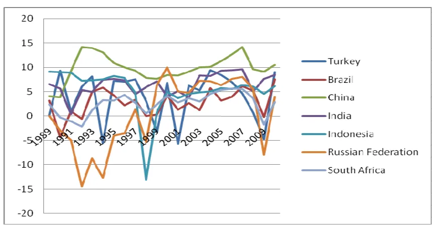
The development of the considered emerging countries was characterised by unsteady

growth of GDP in the 1990s, and by significant declines in the cases of Russia and Indonesia.

All BRIICS countries have followed accelerating positive growth since 2000, with the

exception of Turkey, which had a decline in its real GDP in 2001 with subsequent recovery.

However, it can be seen from Figure 3 that the growth of all BRIICS countries significantly

slowed down in 2009, being affected by the global financial crisis with the extreme case of

Russia, where a decline in real GDP was observed. In terms of the growth of real GDP, the

countries that were least affected by the global financial crisis were China and Indonesia,

while the country that was the most affected was India. After substantial slowdowns, all

Insert Figure 3

A great deal of attention in the literature is spent on the contagion effect of the global

crisis on the financial markets of emerging economies. Aloui et al. (2011) in their paper

on the effect of the global financial crisis in BRIC countries employed a multivariate

copula approach. They demonstrated that the financial markets of countries that are highly

dependent on commodity prices, Brazil and Russia, are more heavily dependent on the

United States compared to such countries as China and India, which are more dependent

on the export prices of finished products. Dooley and Hutchison (2009) in their study

using the decoupling-recoupling hypothesis evaluated the transmission of the U.S. crisis to

emerging markets including the BRIICS and Turkey examples, except for India and

Indonesia. They found that the equity markets of emerging economies appeared to have

been isolated from the U.S. financial markets for the period starting from the date when

the first signals of the crisis appeared in the U.S. until the summer of 2008. However,

starting from the summer of 2008, the financial markets in emerging economies were

found to be highly correlated to the deteriorating economic conditions of the U.S. Thus

studies on the financial transmission of the crisis provide evidence of the moderate

responsiveness of emerging financial markets to the signals of the crisis in the United

States.

However, due to the short time span not enough studies have been completed on

change in trade tendencies in response to the global crisis in the world, including

emerging markets. For example, McKibbin and Stoeckel (2009) studied the potential

impact of the financial global crisis on the world in 15 countries and regions including

developed as well as developing countries by modelling the crisis as a combination of

shocks to a set of changes in an economy. They found that financial crisis caused trade

lead to the deterioration of the domestic and trade partners GDPs. At the same time, the

authors found that financial protectionism emerged as well, enforcing the decline in

international trade flows. Chor and Manova (2010) in their study showed how credit

conditions during the global financial crisis affected world trade flow. They found that

high interbank rates and tight credit conditions were important channels of the

transmission of financial crisis on trade flows.

This study seeks to clarify empirically the consequences of the global financial crisis

in the trade sector of major developing countries. The focus of this study is on the trade

patterns of the developing countries BRIICS and Turkey. This study estimates the effect

of the financial crisis by measuring trade elasticities in export and import demand

functions for two different periods on a quarterly basis, 2007Q2 and

1989Q1-2010Q4. It is known that first signs of the financial crisis took place in August 2007 in the

U.S., followed by a global contagion effect that emerged in the second half of 2008 in

many countries. To measure the trade elasticities of the developing countries two periods

were chosen, the pre-crisis period and the full period including the global financial crisis

and its contagion effect, to be able to capture the changes in trade elasticities that may

have happened before and after the contagion effect started. The financial crisis that

spread in the second half of 2008 generally may be defined as a decline in foreign

investments, changes in foreign debt servicing burdens, a reduction in trade credits and a

global decline in total expenditures.

The paper is structured as follows. The next section highlights the main features of the

pre- and post-crisis trade patterns of BRIICS countries and Turkey. Section 3 explains the

methodology, applied export and import demand functions and outlines the testing

strategy. Section 4 presents and discusses the main empirical results. Finally, Section 5

2. Methodology

To examine to what extent movements in the balance of trade are explained by change

in relative prices, income and exchange rate the imperfect substitute model (Goldstein and

Khan 1985) was employed for the export and import demand functions, where it is assumed

that foreign and domestic products are imperfect substitutes.

Xit = f(Pxit,Pt*,Yt*) (1)

Where t denotes the time period of estimation, Xit is the total export of ithcountry, Pxit

is the export price of ith country in the national currency, Pt* denotes the foreign price

deflator in the national currency of the estimated country, and Yt* is foreign real GDP

expressed in the national currency of the estimated country. The total export in the equation 1

can be measured as total nominal exports deflated by export price index. However there is the

lack of data on export price index on bilateral basis. Therefore, as an alternative, export values

(or inpayments) are used to determine the currency and income changes. If we divide the

right-hand side of equation (1) by foreign prices Pt*, due to the linearity of demand functions

the export demand is not going to change (Goldstein and Khan 1985). Therefore, the

logarithmic form of the export demand function may be expressed in the following form:

LnXit = c0 + c1 Ln(Pxit/Pt*) + c2 Ln(Yt*) + t (2)

Where LnXit is the natural logarithm of the total export value of ith country,

Ln(Pxit/Pt*) is the natural log of relative export prices of the estimated country relatively to

foreign country and Ln(Yt*) is the natural logarithm of the foreign income. Finally t is the

error term.

Due to the difficulty in obtaining the import and export prices of the estimated

countries, equation 2 has to be modified. The modified approach used in the literature is to

those by Bahmani-Oskooee and Economidou (2005), Bahmani-Oskooee and Ratha (2008),

Irandoust et al. (2006), Kwack et al. (2007), and Kumar (2008) and others used real exchange

rates in their studies to calculate the exchange rate elasticity. Therefore, the alternative

log-linear form of the export demand function can be written as follows:

LnXit = 0 + 1 Ln(Et) + 2 Ln(Yt*) + t (3)

Where Et is the real exchange rate calculated by the following formula:

where ER is the nominal exchange rate represented in foreign currency per unit of

domestic currency. As a proxy for domestic and foreign prices a GDP deflator is used (for

similar studies, see Irandoust et al. [2006] and Kwack et al. [2007]). Yt* is the real GDP of the

foreign trade partner. For every estimated country, a set of nine countries is chosen as a

representative of the foreign trade partner. Countries in every set are selected according to the

highest time-varying bilateral trade shares between the estimated country and its trade

partners.2 It is expected that the coefficient of relative export price 1 in equation 3 being

negatively related to export value as an increase in domestic prices will decrease the demand

for export while foreign price increase will raise the demand for export. Income elasticity 2

may get different signs. It will get a positive sign if an increase in the foreign income raises

demand for home country export. However, if foreign goods and services are highly

competitive with home country export foreign income in this case can have negative effect on

the export value from the home country.

2

The standard form of the import demand function can be expressed by the following

equation:

Mit = f(Pmit,Pt,Yt) (4)

Where Mit is the import of ith country, Pmit is the import price of ith country in the

national currency, Ptdenotes domestic price deflatorand Ytis the domestic real GDP. There is

a lack of data on import price index on bilateral basis, similar to export demand equation.

Therefore, import values (or outpayments) are used to determine the currency and income

changes in equation 4. Following the extraction of export demand function the right-hand side

of equation (4) can be divided by domestic prices Pt. As a result, the import demand function

is taking the following form:

LnMit = 0 + 1 Ln(Pmit/Pt) + 2 Ln(Yt) + ut (5)

Where LnMit is the natural logarithm of the total import value for ith country,

Ln(Pmit/Pt) is the natural logarithm of relative import prices, Ln(Yt) is the natural logarithm of

the domestic income. Finally ut is the error term. The log-linear form of the import demand

function corrected for import prices will take the following form:

LnMit = 0 + 1 Ln(Et) + 2 Ln(Yt) + ut (6)

Where Et is the real exchange rate calculated by the following formula:

where ER is the nominal exchange rate represented in domestic currency per

foreign currency. Y is the domestic output. It is assumed that the relative import prices

coefficient 1 will be related negatively to the import quantity as according to the demand

theory increase in the import price will reduce the import demand while increase in domestic

prices will raise demand for import. However, income elasticity 2 can have different signs as

the domestic production, income will have a positive effect on the import volume. However,

if there are a lot of import substitutes in the domestic production, an increase in the domestic

income can lead to a decrease in the import demand.

The focus of the analysis is to study the long-run relationship and dynamic interactions

among the variables in the export and import demand functions. To incorporate the short-run

dynamics, the autoregressive distributed lag (ARDL) approach to cointegration is applied.

The ARDL approach involves two steps for estimating the long-run relationship (Pesaran et

al. 2001). The first step is to examine the existence of long-run relationship among all

variables in an equation and the second step is to estimate the long-run and short-run

coefficients of the same equation. The second step determines the appropriate lag lengths for

the independent variables and is applied only in the case if cointegration relationships are

found in the first step. In error-correction models, the long-run multipliers and short-run

dynamic coefficients improve the export demand function as follows:

+ ∆ + ∆ + ∆ + = ∆ ₋ = − = −

= t i

p i i t p i i t p i

t X E Y

X log log log *

log ₃ 0 2 0 1 1

0

λ

λ

λ

λ

t t t

t

E

Y

X

φ

φ

ε

φ

+

+

+

+

log

log

log

*

The error correction model for the import demand function is as follows:

+ ∆ + ∆ + ∆ + = ∆ ₋ = − = −

= t i

p i i t p i i t p i

t M E Y

M log log log

log 3 0 2 0 1 1

0

µ

µ

µ

µ

t t t

t

E

Y

u

M

+

+

+

+

ϕ

log

ϕ

log

ϕ

log

Equations (7) and (8) may be transformed to following equations in order to accommodate the

one lagged error correction term:

+ ∆ + ∆ + ∆ + = ∆ ₋ = − = −

= t i

p i i t p i i t p i

t X E Y

X log log log *

log ₃ 0 2 0 1 1

0

λ

λ

λ

t t

EC

ε

δ

+

+

+ ∆ + ∆ + ∆ + = ∆ ₋ = − = −

= t i

p i i t p i i t p i

t M E Y

M log log log

log ₃ 0 2 0 1 1

0

µ

µ

µ

µ

t

t

u

EC

+

+

ν

The ARDL approach is used to establish whether the dependent and independent variables

in each model are cointegrated. The null of no cointegration H₀:φ₁=φ₂=φ₃=0 in the export

demand model is tested against the alternative hypothesis ofH₁:φ₁≠φ₂ ≠φ₃ ≠0. In the import

demand function the null of no cointegration H₀:ϕ₁=ϕ₂=ϕ₃=0 is tested against the

alternative hypothesis ofH₁:ϕ₁≠ϕ₂ ≠ϕ₃≠0.

The Walt-type (F-test) coefficient restriction test is conducted, which entails testing the

above null hypotheses H₀ andH₁. Pesaran et al. (2001) computed two sets of asymptotic

critical values for testing cointegration relationships existence. The first set assumes variables

to be I(0), the lower bound critical value (LCB) and the other I(1), upper bound critical value

(UCB). If the F-statistic is above the UCB, the null hypothesis of no cointegration can be

rejected irrespective of the orders of integration for the time series. Conversely, if the test falls

below the LCB, the null hypothesis cannot be rejected. Finally, if the statistic falls between

these two sets of critical values, the result is inconclusive.

Since the results of the F-test are sensitive to lag lengths, we apply various lag lengths in

the model. However, as Pesaran and Pesaran (1997, 305) argue that variables in regression

that are “in first differences are of no direct interest” to the bounds cointegration test. Thus, a

result that supports cointegration at least at one lag structure provides evidence for the

(1998) have demonstrated that in an ECM, significant lagged error-correction term is a

relatively more efficient way of establishing cointegration. So, the error correction term can

be used when the F-test is inconclusive.

3. Empirical Results

a. Cointegration Test

In order to ascertain whether the tested variables are stationary, the ARDL cointegration

test was employed. Based on the cointegration test results represented in Table 1, the strong

evidence of the cointegrating relationship was found in export demand functions in all

countries except India and South Africa. On the other hand, weak evidence for cointegration

was found for the cases of Russia and Indonesia with a 10% significance level. Testing Import

demand functions, the existence of cointegration can be confirmed with 1 and 5% significance

levels in all cases except Brazil, where cointegration was confirmed with a 10% significance

level, while in the case of China the hypothesis of no cointegration was accepted. Therefore,

continuing with further estimations, India and South Africa in export demand function and

China in import demand function cannot be included.

b. Cointegration Coefficient Estimates

The stationarity of the linear combination of a group of non-stationary series is defined

by the cointegration test. In order to find the long-run equilibrium relationship among

variables, the linear combination of the non-stationary time series has to be stationary. The

long-run cointegrating coefficients are estimated by using ARDL procedure, where the

appropriate autoregressive order was chosen by using the Schwarz criterion (SC), and

presented in Table 2. The coefficients 1 and 1 represent long-run elasticities of real exchange

rate for export and import demand functions on the basis of equations 3 and 6, respectively.

function (equation 3), while the coefficients 2 illustrate the long run elasticities of domestic

income for the import demand function (equation 6).

It is assumed in the paper that the real exchange rate coefficients of export and import,

respectively, are related negatively to trade flows. An increase in relative foreign prices may

lead to an increase in export demand. On the other hand, an increase in export prices leads to

a decline in export demand (see equation 2). Whereas in the case of import demand function

a raise in foreign prices leads to a decline in import demand, while an increase in domestic

prices leads to an increase in import demand (see equation 5). The results of long-run

coefficient estimations are presented in Table 2, where India and South Africa are not

included due to the lack of cointegration relationships in the export demand function. From

Table 2 it can be seen that in the export demand function exchange rate elasticities of Turkey,

Brazil, Indonesia and China produced the expected negative sign and only in the case of

Russia was the real exchange rate elasticity estimated with positive sign for the considered

periods. In all cases of the export, demand function exchange rate elasticities appeared to be

inelastic in addition to being very close to zero. However, the majority of exchange rate

estimates did not show significance, which illustrates that the real exchange rate does not

influence the export demand in the considered developing countries in the long run.

Insignificant change in the values of the exchange rate elasticities can be observed

when different estimation periods are compared. Thus in the cases of Brazil, Russia and

Indonesia exchange rate elasticities almost did not show any changes in the period of the

global financial crisis compared to the pre-crisis period 1989-2007. In the case of Turkey, the

exchange rate elasticity of exports declined and appeared to be significant in the period

covering the crisis, thus illustrating the decline of the export responsiveness to prices. In the

the elasticity value is so small and insignificant that it is still illustrates the low responsiveness

of exports to the real exchange changes in the long run.

The results of the estimations are consistent with some results in the literature. For

example, in the case of Turkey, Ozkale and Karaman (2006) concluded that price is inelastic

and the sign of the real exchange rate is negative for the export demand function for goods

trade. While Aydin et al. (2004), on the other hand, found that the exchange rate is inelastic

for goods but a positive in sign in Turkey. Hossain (2009) found as well that the long-run

relative price elasticity of the demand for exports is significantly lower than that in Indonesia.

Vieira and Haddad (2011) found in the case of Brazil that the trade weighted real

exchange rate elasticity of manufactured export is inelastic with expected negative sign.

Algieri (2004) found that in case of Russia the relative prices elasticity of exports is

significant and elastic with expected negative sign, contrary to the results of the present study.

However, the exports of Russia in Algieri (2004) did not include oil, gas or its product. The

inclusion of oil and energy products in exports produced the inelasticity of exports to relative

prices, indicating that the demand for energy products are inelastic to change in prices. On the

other hand, the real exchange rate elasticity in the Chinese export demand function in Cheung

et al. (2009) was found with significant and highly elastic with negative sign. However,

Cheung et al. (2009) in their study use the CPI-deflated exchange rate, which may be a

weaker measure compare to the GDP deflator, and may produce different results.

Thus the export estimation results show that changes in the real exchange rates do not

affect exports in the long run considering the pre-crisis periods and the period that saw the

global financial crisis.

The long-run income elasticities 2 and 2 of export and import, respectively, are

foreign incomes. Respectively, an increase in domestic incomes is expected to increase the

demand for imports, giving positive sign to elasticity. Estimations of the export demand

function provide enough evidence to assume a positive relationship between income and

export demand in all of the considered countries with high significance levels in the majority

of cases. In the cases of Turkey and Brazil, the long-run income elasticities of export demand

function are elastic and significant with positive sign. The results illustrate that the income

elasticities are higher in pre-crisis periods than in the period that experienced the financial

crisis. Thus it can be concluded that the general trend of high export responsiveness to income

slightly declined as a result of the global financial crisis. However, in the cases of Russia,

Indonesia and China, the long-run export responsiveness to foreign incomes increased in the

period which experienced the financial crisis with a high significance level only in the case of

Indonesia.

The statistical data show that Indonesia was one of the first to recover from the global

crisis countries out of the considered countries. Indonesia has the highest growth rate of

exports value in 2010 compare to 2008. If in 2009, all of the considered countries had

significant declines in export trade, in 2010 the exports values of Turkey and Russia were

lower compare to 2008, while in Indonesia the exports value were 15% higher than in 2010.

In second and third place were India and China, where the growth rate was 11 and 10%,

respectively.

The results of the estimations are consistent with those of the literature. For example,

Algieri (2004) found that the world income long-run elasticity of exports is elastic in the case

of Russia. Hossain (2009) in its study found evidence that long-run income elasticity for

Indonesia’s exports is significantly greater than one, which is consistent with the present

study. These results are similar to the outcomes of Cheung et al. (2009) that produce high and

incomes of trading partners proportionally increase export demands for Russian, Indonesian

and Chinese goods.

Accordingly, we have enough evidence to conclude that it is primarily the foreign

income that affects the export demand in the long run in BRIICS countries and Turkey. It is

found that while the tendency of export responsiveness to foreign income decreased in the

cases of Turkey and Brazil in the period when the financial crisis is included, in the cases of

Russia, Indonesia and China there was an increasing tendency in export responsiveness to

foreign income. The trading partners of Turkey and Brazil had slight changes for import

substituted goods, while in the cases of Russia, Indonesia and China trade partners that had a

tendency to increase imports from these countries after the financial crises was included. The

tendency of increased imports may illustrate the comparative advantage of trading goods

compare to local ones, while the global crisis has a negative effect on the competitiveness

level of local production. However, the results illustrate that the trading partners of Turkey

and Brazil prefer an import substitution policy during crises, which significantly decreased the

value of the exports of these countries. These results are supported by statistical data3

demonstrating a 12% decline in export values in 2010 compared to 2008, while in Brazil

export values increased in 2010 only by 2% compared to 2008.

The estimations of the import demand function do not include the case of China due to

the absence of cointegration relationships between variables. The estimates of the long-run

exchange rate coefficients produced an expected negative sign only in the case of Russia,

while in all other cases the long-run exchange rate elasticity appeared to be positive. In all of

the estimated countries the long-run exchange rate elasticity was found inelastic. In the cases

of Brazil, India and Indonesia, the exchange rate elasticities were found inelastic, nearly close

to zero, and they were not found to be significant in the import demand function. Estimates of

3

the long-run exchange rate elasticities of Turkey and South Africa were found to be

significant and inelastic with positive sign.

The depreciation of domestic currency leads to a slight increase in imports indicating

signs of the possible presence of a J curve. The assumption of existence of the J curve effect

in the cases of Turkey and South Africa are verified by results obtained on the exchange rate

elasticities of exports. The depreciation of a currency making exports cheaper to foreign

buyers therefore exports increase and imports decrease. However, in the short run, such

reasons as existing contracts, the inelasticity of exports or imports, the absence of alternative,

do not allow exports or imports to change significantly. In these cases depreciation is

followed by an increase in import values and decrease in export values. In this study,

increases in imports and decreases in exports following depreciation in the cases of Turkey

and South Africa are reflected by long-run coefficients as well, without the indication of

balance of trade improvement in the long run. However, it is important to note that the current

study is carried out on the basis of quarterly data, where the long-run term still may be short

enough to illustrate the balance of trade improvement.

Similar results are found in the literature as well. Ogus and Sohrabji (2009) found that

the exchange rate has a negative effect on Turkish exports; however, they found that the

exchange rate has negative effects on imports as well. Aydın et al. (2004) found that real

depreciation will not increase exports significantly; however, in their study they found that

depreciation will decrease the volume of imports significantly. Narayan and Narayan (2003)

found relative prices of elasticity of demand in South Africa inelastic as well; however, with

negative sign. The values of the long-run exchange rate elasticities in the cases of Turkey and

South Africa were found to be similar in the estimated pre and post crisis periods, providing

additional evidence of the exchange rate insignificance in the long run for the considered

with expected negative sign indicating that the depreciation or appreciation of the Russian

ruble leads to a decrease or increase in imports, respectively. However, the inelasticity of the

exchange rate indicates that changes in imports that take place due to the real exchange rate

fluctuations are not major. On the other hand, it can be seen that the real exchange rate

appeared to be more inelastic and insignificant in the period which covered the global

financial crisis.

All coefficient estimates of income for import demand function were found to be

elastic with positive sign. In most of the estimated countries long-run income elasticities were

found statistically significant. The positive sign of income elasticity shows that with an

increase in income, the estimated countries have higher preferences for imported goods than

for domestic ones. In all of the estimated countries, except South Africa, the values of

long-run income elasticities demonstrate increase in the period which covered the global financial

crisis. This indicates that the global crisis did not deteriorate demand for imports in the

considered developing countries; conversely it shows an increasing tendency in demand

growth for import in response to growing domestic incomes. The period 1989-2010, which

demonstrates an increase in long-run income elasticities, was characterised by sharp declines

in domestic incomes in all of the considered countries at the end of 2008 and at the beginning

of 2009 (see Figure 3). Therefore, increased income elasticities may be interpreted as a rising

tendency in import decline in response to declining domestic real incomes during the global

financial crisis. Estimates of the long-run income elasticities of South Africa reveal a decline

in the period covering the crisis indicating a slight decline in the import demand response to

income changes.

In general, there is enough evidence to conclude that the real exchange rate does not

significantly affect the export and import demands in the long run in the estimated developing

and Brazil, the export demand response to foreign income changes declined in the period

covering the global crisis. This indicates that the global financial crisis slightly directed the

trading partners of Turkey and Brazil towards import substituting policies, or towards cheaper

producers; however, these changes were not major. In Indonesia, the response of export

demand to changes in the foreign incomes increased, indicating that as a result of an effect of

the financial crisis, an increase or decrease in foreign income led to a higher increase or

decrease in export demand, respectively. The estimations provide enough evidence of high

dependence on the import demand function on the domestic income in the long run. The

estimations illustrate that the import demand became more sensitive to changes in domestic

income after the effect of the global crisis in Turkey, Brazil, Russia, India and Indonesia,

while the level of dependence of imports on domestic incomes slightly declined in South

Africa.

c. Error Correction Model

The vector error correction model is designed for cointegrated series. The vector error

correction model specifies the short-run adjustment dynamics for long-run equilibrium

deviations. The results of the short-run coefficient estimates associated with the long-run

relationships obtained from the ECM version of the ARDL model are presented in Table 3.

The ECM coefficient is supposed to be significant with negative sign indicating the speed of

the adjustment of variables to the long-run equilibrium. Error correction terms δ_{1 for the}

export and ν₁for the import demand functions, respectively, were found negative and

statistically significant in the case of Indonesia in the first period of the export demand

function and in Turkey, Brazil and Indonesia in the second period. Estimating the import

cases of Turkey, Russia and South Africa in the first period and in Turkey, India, Indonesia

and South Africa in the second period. These results ensure once more that stable long-run

relationships among the variables in the model of current account balances exist in all

considered countries, as noted by Kremers et al. (1992) and Bannerjee et al. (1998).

The magnitude of the error correction term in the export demand function is between

-0.019 and -0.108, depending on the estimated country in the first period, and between -0.021

and -0.115 in the second period. Therefore, it implies that disequilibria in the export demand

function was corrected by approximately 2-11% every quarter (respective to country) before

the global financial crisis. This means that a steady state equilibrium in the export demand

function can be reached between 2 and 13 years, respective to country in the pre crisis period.

However, in the period covering the crisis, the general tendency of the disequilibria correction

almost did not change, the steady state equilibrium was reached in the period between 2 and

12 years, respective to country. Only some slight changes were observed on the individual

country level. Thus, in Turkey, the steady state equilibrium was reached in approximately 6

years in the pre crisis period, while under the effect of the global crisis this period declined to

2 years.

In the import demand function the equilibrium adjustment speed is higher compare to

export functions. Thus the magnitude of the error correction term is between 0.055 and

-0.296 in the pre crisis period and between -0.055 and -0.294 in the full period. Therefore the

steady state equilibrium can be reached in the period between less than a year and four and

half years. Particularly in Turkey the steady state equilibrium was reached in less than a year

with no effect from the global crisis, while in South Africa the adjustment process declined

Signs of the short-run elasticities are consistent with those of the long-run elasticities

signs from Table 2. Strong support was found for concluding that the short-run exchange rates

do not play a very important role in the long-run behaviour of import and export demands. In

contrast to studies on export and import demand functions for services, where for example

Ketenci and Uz (2010) in the example of Turkey found that short-run exchange rate

elasticities of export and the import of services are highly elastic compared to inelastic

long-run exchange rate elasticities. In all countries, the short long-run exchange rate elasticities in export

as well as in import demand functions were found highly inelastic, nearly close to zero. Thus,

only 0.1% of the disequilibrium of import in Turkey is corrected by exchange rate, and only

0.01 % of the disequilibrium of export in China is corrected by exchange rate. In contrast to

studies on export and import demand functions for services, where, for example, Ketenci and

Uz (2010) in the example of Turkey found that short-run exchange rate elasticities of export

and import of services are highly elastic compare to inelastic long-run exchange rate

elasticities.

Signs of the short-run income elasticities are consistent with signs of the long-run

income elasticities in export as well as in import demand functions, except for the case of

Turkey, where the short-run foreign income elasticity appeared with negative sign indicating

that with an increase of income, foreign countries follow import substitution policies.

However, the short-run income elasticity in the case of Turkey was not found significant;

therefore, the conclusion cannot be certain. Estimations of the export demand function

illustrate that in all countries except China the short-run foreign income is inelastic,

demonstrating that on average about 20% of the disequilibrium in the export was adjusted by

foreign income in the pre crisis period in the considered developing countries. On the other

hand, the global financial crisis increased the importance of foreign income for export

export, respectively to a country, was adjusted by foreign income. In the case of China,

foreign income was found to be highly important for export demand with increasing tendency

after the crisis. Thus more than 300% disequilibrium in export was adjusted by foreign

incomes in the pre-crisis period, while under the effect of the global crisis foreign income was

responsible for adjustment of 400% of disequilibrium in export.

Estimations of the short-run income elasticities in the import demand function

provided highly statistically significant results in all countries. In all countries, the global

crisis increased the importance level of domestic incomes in the import demand function by

increasing the value of the short-run income elasticities. The extreme case is South Africa,

where before the crisis about 70% of the disequilibrium in imports was adjusted by domestic

income, while with the effect of the crisis domestic income became responsible for more than

500% of the disequilibrium in imports, illustrating the steep increase in the import demand

sensitivity level to domestic incomes in South Africa. In other words, when deviations from

the long-run equilibrium occur in the export and import demand functions of selected

countries, it is primarily the foreign and domestic incomes that adjust to restore long-run

equilibrium each quarter in the export and import demand functions, respectively, rather than

the real exchange rate.

4. Conclusion

This paper empirically examined the effects of financial crisis on changes in the trade

elasticities of BRIICS (Brazil, Russia, India, Indonesia, China and South Africa) countries

and Turkey. The effect of the financial crisis was estimated by measuring trade elasticities in

export and import demand functions for two different periods on the quarterly basis:

1989Q1-2007Q2 and 1989Q1-2010Q4. The first period was the pre-crisis period and second was the

were studied in order to capture the changes in trade elasticities happened before and after the

contagion effect started.

The empirical results provide strong support for concluding that short-run exchange

rates do not play a very important role in the long-run behaviour of import and export

demands. In all of the estimated countries, except China, the short-run foreign income was

found inelastic with increasing tendency under the effect of the global crisis. The short-run

income elasticities in the import demand function were found highly statistically significant

and elastic in all countries. The results indicate that in all estimated countries the global crisis

increased the importance level of domestic incomes in import demand.

The empirical results of long-run coefficients provide enough evidence to conclude

that changes in the real exchange rate do not significantly affect the export and import

demands in the long run. On another hand, foreign and domestic incomes were found highly

significant and elastic in export and import demand functions. In Turkey and in Brazil, the

responsiveness of export demand to foreign income declined after the global crisis. This

indicates that the global financial crisis slightly directed the trading partners of Turkey and

Brazil towards import substituting policies or towards cheaper producers. In Indonesia, the

global financial crisis increased the sensitivity of export demand to changes in foreign

incomes. Indonesia is one of a few countries that did not negatively affected by the financial

crisis. Indonesia increased its global market share and domestic sales as well. This increase in

exports is mainly attributable to resource based commodities, while there is still limited

progress in exports of manufactured products4.

The empirical results illustrate the high dependence level of the import demand

function on the domestic income in the long run. Thus the import demand became more

4

sensitive to changes in the domestic income as a result of the global crisis effect in Turkey,

Brazil, Russia, India and Indonesia, while the level of the dependence on imports on domestic

incomes slightly declined in South Africa.

In general, the responsiveness of exports and imports to the exchange rate in the

considered emerging markets was very low and in many cases insignificant, where the global

crisis did not have any effect on these relationships. On the other hand, the crisis in most of

countries increased the already high responsiveness of exports and imports to foreign and

domestic incomes, respectively. Taking into account that the incomes in the world improved

after the crisis and started to increase in 2009 and 2010, it can be concluded that recovering

from the crisis’s negative effects emerging countries and their partners did not close their

countries, but followed the tendency of international trade increase. Therefore, the trade

policies of emerging countries should be based mainly on foreign and domestic incomes. The

further research has to include extended dataset that will be helpful in estimation of the effect

5. References

Algieri, B. 2004. Price and income elasticities of Russian exports. The European Journal of

Comparative Economics1 (2): 175-193.

Aydin, M.F., Ciplak, U., and Yucel, M.E. 2004. Export supply and import demand models for

the Turkish economy. Research Department, Working Paper 04/09. The Central Bank

of the Republic of Turkey.

Aloui, R., Aïssa, M.S.B. and Nguyen, D.K. 2011. Global financial crisis, extreme

interdependences, and contagion effects: The role of economic structure? Journal of

Banking & Finance35: 130-141.

Bahmani-Oskooee, M., and Economidou, C. 2005. How sensitive are Britain’s inpayments

and outpayments to the value of the British pound. Journal of Economic Studies 32:

455-467.

Bahmani-Oskooee, M., and Ratha, A. 2008. Exchange rate sensitivity of US bilateral trade

flows. Economic Systems32: 129-141.

Banerjee, A., Dolado, J. J., Mestre, R., 1998. Error-correction mechanism tests for

cointegration in a single equation framework. Journal of Time Series Analysis19:

267-283.

Goldstein, M., and Khan, M. 1985. Income and price effect in foreign trade. In Handbook of

International Economics. Jones, R.W., Kenen, P.B. (Eds.). Amsterdam, North Holland, pp. 1042–1099.

Cheung, Y.W., Chinn, M.D. and Fujii, E. 2009. China’s Current Account and Exchange Rate.

NBER Working Paper 14673. Cambridge.

Chor, D. and Manova, K., 2010. Off the Cliff and Back? Credit Conditions and International

Trade During the Global Financial Crisis. NBER Working Paper 16174, Cambridge.

Dooley, M., and Hutchison, M. 2009. Transmission of the U.S. subprime crisis to emerging

markets: Evidence on the decoupling-recoupling hypothesis. Journal of International

Money and Finance28: 1331-1349.

Hossain A.A. 2009. Structural change in the export demand function for Indonesia:

Estimation, analysis and policy implications. Journal of Policy Modelling31(2):

260-271.

Irandoust, M., Ekblad, K., and Parmler, J. 2006. Bilateral trade flows and exchange rate

sensitivity: Evidence using likelihood-based panel cointegration. Economic Systems30

(2): 170-183.

Ketenci, N. and Uz, I. 2010. Trade in Services: The elasticity approach for the case of Turkey.

The International Trade Journal24 (3): 261-297.

Kremers, J. J. M., Ericsson, N. R., Dolado, J. J., 1992. The power of cointegration tests.

Oxford Bulletin of Economics and Statistics54 :325-348.

Kumar, S. 2008. An empirical evaluation of export demand in China. Journal of Chinese

Economic and Foreign Studies2 (2): 100-109.

Kwack, S.Y., Ahn, C.Y., and Yang, D.Y. 2007. Consistent estimates of world trade elasticities and an application to the effects of Chinese Yuan (RMB) appreciation.

Journal of Asian Economics18 :314-330.

McKibbin W.J. and Stoeckel, A., 2009. The Potential Impact of the Global Financial Crisis on

World Trade. Policy Research Working Paper 5134. The World Bank.

Narayan, S. and Narayan, P.K. 2003. Import Demand Elasticities for Mauritius and South

Africa: Evidence from two recent cointegration techniques. Discussion papers 03/09,

ISSN 1441-5429. Monash University, Department of Economics.

Ogus, A. and Sohrabji, N. 2009. Elasticities of Turkish Exports and Imports. Working Paper,

0906, Izmir University of Economics.

Ozkale, L., and Karaman, F.N. 2006 (in Turkish). Static effects of the EU-Turkey customs union. International Economics and Foreign Trade Policies. Undersecretariat of the Prime Ministry for Foreign Trade.

Pesaran, M. H., Shin, Y. and Smith, R. C., 2001. Bounds testing approaches to the analysis of

Pesaran, M. H. and Pesaran, B. 1997. Working with Microfit 4.0: Interactive Econometric Analysis. Oxford University Press, Oxford.

Vieira, F.F. and Haddad, E.A. 2011. A panel data investigation on the Brazilian state level

export performance. TD Nereus, 12-2011. Sao Paulo.

Figure 1. Exports in billions of US dollars

Source: Calculations are made on the basis of OECD statistics

Figure 2. Imports in billions of US dollars

Figure 3. Real GDP, Growth Rate

Source: Calculations are made on the basis of OECD statistics

Table 1. F-statistics for testing cointegration relationship

EXPORT IMPORT

Country Lags F-statistic Probability Lags F-statistic Probability

Turkey 6 F(3,57)= 2.887* 0.043 6 F(3, 57)= 4.005** 0.012

Brazil 4 F(3, 65)= 3.356** 0.024 6 F(3, 57)= 2.534 0.066

Russia 1 F(3, 77)= 2.261 0.088 5 F(3, 61)= 3.268** 0.027

India 4 F( 3, 65)= 1.313 0.278 1 F(3, 77)= 3.703** 0.015

Indonesia 1 F(3, 77)= 2.684 0.052 3 F(3, 69)= 4.026** 0.011

China 6 F(3, 57)= 4.551** 0.006 6 F(3, 57)= 0.208 0.890

South Africa 6 F(3, 57)= 1.004 0.398 6 F(3, 57)= 8.359* 0.000

Table 2. Cointegration Coefficient Estimates (long run) 1989-2010

Export Coefficients lag 1989-2007 lag 1989-2010

Turkey 1 (3,0,1) -0.038 (0.041) (1,0,1) -0.014** (0.006)

2 6.128* (3.685) 3.979*** (0.403)

Brazil 1 (1,0,0) -0.002 (0.002) (1,0,0) -0.002 (0.0009)

2 5.478* (2.957) 4.852*** (1.087)

Russia 1 (1,1,0) 0.008 (0.018) (1,1,0) 0.003 (0.010)

2 2.673 (2.859) 3.158 (1.957)

India 1 - -

2 - -

Indonesia 1 (1,0,0) -0.002 (0.003) (1,0,0) -0.003 (0.003)

2 1.909*** (.3656) 2.250*** (0.311)

China 1 (1,0,1) -0.0001** ( 0.00006) (1,0,2) -0.008 (0.008)

2 3.429** (1.475) 14.570 (9.706)

South Africa 1 - -

2 - -

Import

Turkey 1 (1,0,2) 0.004** (0.002) (1,1,1) 0.005**(0.002)

2 2.995*** (0.141) 3.192*** (0.111)

Brazil 1 (2,0,3) -0.00001 (0.002) (2,0,4) 0.00043 (0.001)

2 2.134 (2.062) 2.428** (1.198)

Russia 1 (1,0,0) -0.019*** (0.007) (1,0,2) -0.001 (0.013)

2 1.327** (0.543) 2.927 (2.184)

India 1 (1,0,0) 0.0002 (0.0004) (1,0,0) 0.003 (0.003)

2 0.184** (0.079) 2.161*** (0.249)

Indonesia 1 (3,0,1) 0.00003 (0.004) (3,0,1) 0.001 (0.004)

2 1.481*** (0.465) 2.133*** (0.412)

China 1 - -

2 - - -

South Africa 1 (1,0,0) 0.055** (0.023) (1,0,1) 0.056** (0.025)

2 4.508*** (0.914) 3.109*** (0.643)

Notes : *, **, *** indicate significance at 10%, 5% and 1% levels, respectively; standard errors for the coefficient estimate are given in parenthesis. 1 and 1 are the elasticities of exchange rates for export and import from equations 3 and 6, respectively.

Table 3. Vector Error Correction

1

δ 2 3

1

δ 2 3

Export 1989-2007 _1989-2010

Turkey -0.039 (0.048)

-0.002 *** (0.0006) -0.279 (0.262) -0.115*** (0.043) -0.002** (0.0007) -0.039 (0.227)

Brazil -0.052 (0.047)

-0.0001 (0.0001) 0.283* (0.172) -0.082** (0.039) -0.0001 (0.0001) 0.398 ** (0.165) Russia -0.066 (0.071) 0.005** (0.002) 0.176 (0.118) -0.099 (0.069) 0.005** (0.002) 0.313** (0.124)

India - - - -

Indonesia -0.108** (0.053)

-0.0002 (0.0003) 0.207*** (0.119) -0.115** (0.047) -0.0003 (0.0003) 0.259** (0.118)

China -0.019 (0.032)

-0.0001 ** (0.0001) 3.429** (1.475) -0.021 (0.023) -0.0002*** (0.0001) 3.989*** (1.021) South

Africa - - - -

Import ν1 2 3 ν₁ 2 3

Turkey -0.296*** (0.079)

0.001** (0.0006) 3.079 *** (0.300) -0.294*** (0.072) -0.003* (0.002) 2.902 *** (0.267)

Brazil -0.055 (0.058)

-0.000 (0.0001) 2.838*** (0.535) -0.055 (0.044) 0.000 (0.0001) 3.223*** (0.459)

Russia -0.127** (0.054)

-0.002*** (0.001) 0.168*** (0.088) -0.065 (0.055) -0.0001 (0.001) 0.942** (0.468)

India -0.068 (0.043)

0.0002 (0.0004) 0.184** (0.079) -0.135*** (0.039) 0.0004 (0.0004) 0.292*** (0.084)

Indonesia -0.115 (0.072)

0.000003 (0.0004) 1.738*** (0.548) -0.106* (0.056) 0.0001 (0.001) 1.771*** (0.591)

China - - - -

South

Africa -0.155** (0.061)

0.008** (0.004) 0.696*** (0.228) -0.069*** (0.023) 0.004* (0.002) 5.738*** (0.044)

Notes: *, **, *** indicate significance at 10, 5, and 1 percent levels, respectively. Standard errors are in parentheses.