Munich Personal RePEc Archive
The Signaling Role of Not Being
Promoted: Theory and Evidence
Jin, Xin
University of South Florida
2014
Online at
https://mpra.ub.uni-muenchen.de/58512/
The Signaling Role of Not Being Promoted:
Theory and Evidence
∗Xin Jin
September 9, 2014
Abstract
This article studies the negative signals associated with non-promotion. I first
show theoretically that, when workers’ productivity rises little with additional years
on the same job level, the negative signal associated with non-promotion leads to
wage decreases. On the other hand, when additional job-level tenure leads to a
sizable increase in productivity, workers’ wages increase. I test my model’s
pre-dictions using the personnel records from a large US firm from 1970-1988. I find
a clear hump-shaped wage-job-tenure profile for workers who stay in the same job
level, which supports my model’s prediction.
Keywords: Asymmetric Information, Human Capital Accumulation, Signaling,
Pro-motion, Wages
JEL: J24, J31, M51
∗Corresponding author: Xin Jin, Department of Economics, University of South Florida, Tampa,
Promotion sends positive signals about a worker’s ability and productivity. This
theoretical possibility has been extensively studied in a body of literature stemming
from Waldman (1984a). Waldman assumes that a worker’s current employer has
better information about a worker’s true ability from observing this worker at work.
Potential employers can only infer the worker’s ability by observing her current
period’s job assignment made by her current employer. Waldman’s two main
con-clusions are (1) promotions send positive signals about workers’ abilities and thus
are associated with substantial wage increases; (2) firms promote fewer
employ-ees than what is socially optimal and this distortion is more severe when workers’
human capital is general rather than firm specific.
While the signals associated with promotion have been extensively examined,
the signals associated with non-promotion, on the other hand, are surprisingly
un-derstudied. In this article, I extend the promotion-as-signal framework by arguing
that additional years of job-level tenure (i.e., non-promotion) sends negative signals
about a worker’s ability. Intuitively, if a worker stays in the same job level for many
years while her peers are all promoted, this worker is believed to be less
compe-tent (or is less likely to be a productive worker). These negative beliefs eventually
translate into small wage increases or even wage decreases.
Although the basic idea is intuitive, formal theoretical models that explore this
negative signaling idea are almost non-existent. Bernhardt (1995) is the only
pre-vious study that captures the negative signals associated with not being promoted.
In that study, Bernhardt argues that there is a negative sorting in promotion such
that abler workers are promoted earlier. However, that analysis makes ambiguous
dy-namics. In this article, I build a T-period model with two job levels to explore the
negative signaling role of non-promotion on workers’ wage dynamics.
My model shows that when a worker stays in the same job level for a long
time, her wages first increase then decrease with additional job-level tenure. To see
the logic, consider a set up where a worker’s productivity is jointly determined by
her expected ability and on-the-job human capital accumulation. Firms use
non-promotion as signals to infer workers’ abilities. If firms keep on receiving negative
signals about a worker’s ability from non-promotion, this worker is perceived less
likely to be a productive worker. The negative signals associated with additional
job-tenure eventually cause the non-promoted workers’ wages to fall since
produc-tivity rises little with additional job-level tenure after the worker spends a long time
on the same job. But since human capital accumulates very fast when a worker
first starts on a job, the fast human capital accumulation outweighs the downward
adjustment (due to non-promotion) in beliefs about a worker’s expected ability and
therefore the non-promoted workers’ wages rise with job-tenure even though there
is negative learning about their abilities.
From the above reasoning, if one only considers the learning component in the
wage determination process, wages should decrease with additional job-tenure. On
the other hand, if one only considers the human capital component, wages should
increase then flatten out with additional tenure on the same job. By bringing
to-gether the learning argument and human capital theory, I can explain two wage
patterns observed in Baker et al. (1994a). First, pre-promotion wages increase
then decrease with job-level tenure. Second, the wages in the periods of promotion
This article contributes to the literature in several different ways. First, it fills
a gap in the learning literature by capturing the negative signaling role of
non-promotion. Second, it contributes to the human capital literature by exploring the
relationship between wages and job-level tenure. Third, it provides an explanation
for a set of empirical findings that are not well captured in existing models. It also
provides empirical evidence that is consistent with my model’s predictions.
The outline of the article is as follows. The next section reviews the related
literature. Section 2 sets up the model. In Section 3, I first analyze a T-period
model with full information then compare equilibrium behavior in this benchmark
model to equilibrium behavior in a model with asymmetric information. I present
empirical evidence in Section 4. Section 5 concludes.
1
Related Literature
This article connects two theoretical building blocks in the existing literature on
wage and career dynamics inside firms - learning and on-the-job human-capital
accumulation.
The learning literature falls into two broad categories. One set of papers
as-sumes symmetric learning where workers’ outputs are observed by all firms in the
market (Harris and Holmstrom, 1982). The other set of papers assumes asymmetric
learning where a worker’s current employer privately observes the worker’s output.
The asymmetric learning literature further divides into two areas of focus. One set
of papers investigates the adverse selection issue in labour market turnover
signals following Waldman (1984a). My paper builds on the promotion-as-signal
approach under asymmetric learning.
The promotion-as-signal approach has been extended in many different ways.
Ricart-i-Costa (1988) considers a two-periodn-job-level model. Bernhardt (1995)
considers a two-level model with infinite periods. In Zabojnik and Bernhardt (2001),
a promotion signal contains information about workers’ human-capital investment
rather than their innate ability. DeVaro and Waldman (2012) consider how
pro-motion signals vary with education.1 The promotion-as-signal approach has also been extended to analyze up-or-out contracts and turnover (Bernhardt and Scoones,
1999; Ghosh and Waldman, 2010).
While Waldman (1984a) and the various extensions capture many stylized facts
about wage and promotion dynamics, such as large wage increases upon
promo-tion (Bernhardt, 1995) and the wage-and-firm-size effect (Zabojnik and Bernhardt,
2001), etc., these studies have almost exclusively focused on the positive signals
as-sociated with promotion. My paper fills a gap in the learning literature by exploring
the negative signals associated with non-promotion.
Another important perspective concerning workers’ wage and career dynamics
inside firms is on-the-job human-capital acquisition. Numerous empirical studies
have investigated the contribution of firm tenure and total labour market
experi-ence to individuals’ wage growth and find a concave wage-firm-tenure profile using
household surveys (Altonji and Shakotko, 1987; Topel, 1991; Altonji and Williams,
2005; Sullivan, 2010; Pavan, 2011).2 On the other hand, using a 1% sample of the
1DeVaro and Waldman (2012) treat education as a measure of initial human capital stock, not as
another source of signals.
2Sanders and Taber (2012) provide a comprehensive survey of the literature on life-cycle wage
British labour force, Devereux et. al. (2013) find a hump-shaped relation between
wages and job-tenure when they do not control for firm-tenure.3 Using firms’ per-sonnel records, Baker at al. (1994a) also find a hump-shaped wage-job-tenure
pro-file for non-promoted workers, i.e., their wages first increase with job-tenure then
decrease.
While the standard human capital accumulation theory explains the increase of
wages with job-tenure when workers are new to a job, it does not explain why wages
fall when workers stay on the same job for a long time. The asymmetric learning
framework with human capital accumulation in Waldman (1984a) might potentially
explain the hump-shaped wage-job-tenure relation, however, neither the original
’84 model nor most of the later extensions in the promotion-as-signal literature
capture the negative signals of non-promotion. There are two reasons. First, those
models assume that a worker’s current employer learns about the worker’s ability
perfectly after one period of employment. Second, many of those models have a
strong “winner’s curse” in their equilibrium (Milgrom and Oster, 1987). In models
with asymmetric learning, firms only observe the job assignments of the workers
at other firms (they observe the output of their own workers). When the winner’s
curse occurs, the wage offer that a firm is willing to make to a non-promoted worker
at another firm is determined by the lowest possible expected ability level among
workers with the same job assignment history. Furthermore, this lowest expected
ability does not vary with job-level tenure for the non-promoted worker if the
cur-3They find a negative relation between job tenure and wages holding firm tenure constant. But
rent employer learns the worker’s ability perfectly after a period. Thus, the signal
associated with non-promotion does not cause further adjustments in wage offers
to previous employees and thus wages actually paid.4 My model moves away from the strong winner’s curse problem by assuming the existence of exogenous turnover
as in Greenwald (1986). With exogenous movers, outside firms are willing to offer
wages that are above the expected productivity of the lowest ability worker with a
certain job assignment history. That is, there are further adjustments in wages when
a non-promotion is observed.
The only previous paper that captures negative signals associated with
non-promotion is Bernhardt (1995). Bernhardt considers a framework with human
cap-ital accumulation and asymmetric learning without the winner’s curse. However,
his model predicts that the non-promoted workers’ wages can either increase or
de-crease with additional tenure but the relationship is monotonic. In addition,
Bern-hardt focuses on the relationship between wages and firm-tenure. However, the
household surveys show that workers’ wages do not fall overall with firm-tenure.
As shown in Baker et al. (1994a), workers’ wages only fall with job-tenure when
they stay a long time on the same job level.
In summary, most of the existing promotion-as-signal models do not capture the
negative signals of non-promotion. The only theoretical model capturing this idea
makes predictions that do not match the evidence. By combining the asymmetric
learning argument and human capital theory, I develop a tractable framework to
4In Waldman (1984a), the output on the lower level job is assumed to be a constant. Thus, we
capture a set of empirical findings in Baker et al. (1994a). In particular, Baker et al.
show that, for a worker who stays in the same job level for more than six years, her
wages first increase then decrease. In addition, if a worker earns a promotion within
four or five years of entering into a job level, her wage in the period of promotion is
higher than the promotion wage paid to a worker who was promoted in the previous
period. But if the promotion is more than four or five years after entering into the
job level, her wage upon promotion is lower than the promotion wage paid to a
worker who was promoted in the previous period.
2
The Model
In this section, I set up a T-period model to analyze the role of non-promotion on
workers’ wage dynamics.
There is free entry into the market. All firms are identical with two job levels.
The manager jobs (m) are on the upper level and the labourer jobs (l) are on the
lower level .
Workers enter the labour market in period 1. They are either good (g) or
ordi-nary (r). LetAdenote workers’ ability types, i.e.,A∈ {g,r}. Neither the firms nor
the workers themselves observe the true type of a particular worker. However, their
prior belief is that a worker is good with probability p0. I assume p0is sufficiently
small that, given the production function defined below, all workers are assigned to
the labourer job in period 1.
Outputs are jointly determined by workers’ ability types and their human
realizations. This is a generalization of the setting in previous papers such as
Wald-man (1984a) and Bernhardt (1995) where a worker’s current employer learns about
the worker’s ability perfectly after a single period of employment. Human capital
accumulates deterministically with tenure.
In each period, workeriattains high (H) productive efficiency with probability
θi=θA ∈ {θg,θr}and low productive efficiency with probability 1−θi. That is, a
worker’s ability type affects the probability of attaining high productive efficiency
and a good worker attains high productive efficiency with a higher probability, i.e.,
θg>θr. The high or low production efficiency translates into different output
real-izations on different job levels. To be specific, workeri’s output in periodt if she is
assigned to job jis
yitj =
(1+st)[zHj +f(xit)] with prob. θi
(1+st)[zLj+f(xit)] with prob. (1−θi),j∈ {l,m}.
(1)
I assume zmH >zlH >zlL >zmL >0. This set up captures that the manager job
has greater returns to the high productive efficiency but the labourer job has greater
returns to the low productive efficiency. It also follows the standard assumption
in the job assignment literature as in Sattinger (1975) and Rosen (1982) that the
manager job has greater marginal returns to an increase in the productive efficiency
from low to high.
In addition, I assume that a good worker is on average more productive on the
manager job than on the labourer job but an ordinary worker is on average more
productive on the labourer job than on the manager job. LetEAj=θAzHj +(1−θA)zLj,
has a comparative advantage producing as a manager but an ordinary worker has a
comparative advantage producing as a labourer (although a good worker is always
more productive than an ordinary worker on both jobs, i.e., Egj >Erj,j∈ {l,m}).
Therefore, firms have an incentive to (correctly) assign a good worker to a manager
position and an ordinary worker to a labourer position.
I refer to a worker’s previous period’s employer as the incumbent firm and all
other firms as outside firms. LetqINCit denote an incumbent firm’s belief in periodt
that workeriis good based on her output history.5 Since the speed of learning on the lower level and the upper level job is the same, the belief that a worker is good
is a function of whether or not a worker attains high (low) productive efficiency
only. That is, at which job level she has worked is irrelevant. In addition, given the
binary ability types, only the total number of high (or low) productive efficiencies
that a worker attains matters for the belief in a given period. Let hti−1 denote the
total number of high productive efficiencies that workerihas attained up to period
t−1. The expected output of workeriwho is believed to be good with probability
qit(hti−1)and who is assigned to job jin periodtis
E[yitj|qINCit (hti−1)] = (1+st){qitINC(hti−1)[θgzHj + (1−θg)zLj] (2)
+ [1−qINCit (hti−1)][θrzHj + (1−θr)zLj] + f(xit)}
= (1+st){qINCit (hti−1)Egj+ [1−qit(hti−1)]E j
r +f(xit)},j∈ {l,m}.
xit is worker i’s labour market experience up to periodt. f(·) is the human
5Outside firms’ beliefs about workers’ ability types are based on workers’ job assignments at
capital accumulation function. Following Acemoglu and Pischke (1998), I
as-sume f to be twice continuous differentiable, strictly increasing, concave with
f(0)≥ 0,lim
x→1f
′
(x) = ∞ and lim
x→¯tf
′
(x) =0 for some 2≤t¯≤ T−1. That is,
hu-man capital accumulates very fast when tenure is low. When tenure is higher than
¯
t, human capital almost stops growing with additional tenure. The human capital
accumulation function enters into the production function additively to the part of
the output that is determined by workers’ innate abilities.
st=S>0 if a worker is employed by her previous period’s employer in periodt.
st=0 otherwise. stthus captures firm-specific human capital. Following Bernhardt
(1995), I assume that once a worker leaves her previous employer, her previous
employer becomes a new firm to her and cannot collect the firm-specific human
capital anymore unless she comes back and works for her previous employer for
another period. This assumption guarantees that in each period only one firm can
collect the firm-specific human capital from a worker’s productivity. This means
that workers do not have an incentive to constantly change employers to enable the
firm-specific human capital in multiple firms. In practice, it is possible that after an
employee leaves a firm, the firm’ policy, structure, or business practices change such
that the previous firm-specific human capital is not applicable when this employee
re-enters the firm.
There is a cutoff belief that a worker is good, q∗, such that the expected output
on level l and that on level m are equal. Note that the equal-productivity cutoff
at an outside firm is equal to the equal-productivity cutoff at an incumbent firm.6
6In general, if the firm-specific human capital term is not multiplicative in the production
q∗solvesq∗Egl+ (1−q∗)Erl =q∗Egm+ (1−q∗)Erm, q∗= (Erl−Erm)/[(Egm−Erm)−
(Egl−Erl)]. Thus, if the belief that a worker is good in periodt is above this cutoff
level, she is expected to be more productive on the management job; otherwise, she
is expected to be more productive on the labourer job.
Following Greenwald (1986), I assume that a small fraction,λ, of workers leave
the incumbent firm for exogenous reasons in each period. The existence of
exoge-nous job switchers alleviates the winner’s curse problem as discussed in the
previ-ous section.7 I consider equilibrium behavior whenλ →0.
To keep the model tractable, I focus on parameterizations that satisfy the
fol-lowing two conditions.
(i) q∗<qiT(1).This condition says that if workeri attains only one high
pro-ductive efficiency in any of the previousT−1 periods, she is more productive on
the upper-level job in periodT. Therefore, there are no demotions in equilibrium.
(ii) Sis “large". In particular, I assume that S is large enough (the precise
pa-rameter restriction can be found in the Appendix) that, in periodT, the incumbent
firm has an incentive to assign a worker with only one high output realization up
to period T−1 to the upper level job. This condition guarantees that a worker is
promoted when a high productive efficiency is attained. It also means an incumbent
firm’s belief about a non-promoted worker’s ability type based on realised outputs
is the same as an outside firm’s belief about this worker’s ability type based on
ob-served job assignments. It guarantees that there is promotion in every period and
7Note that the exogenous job-switching status is different in every period, i.e., an exogenous
there is no distortion in firms’ promotion decisions.
Firms and workers are risk neutral and discount the future with a common
dis-counting factorβ <1. There is no cost to workers from changing firms or to firms
from hiring or firing workers. Under these assumptions, long-term contracts are not
necessary, so I consider equilibrium wages that are determined by spot-market
con-tracts. At the beginning of each period, firms engage in a wage-setting game where
they place wage “bids” in order to attract workers. That is, wages are promised
before production begins in each period.
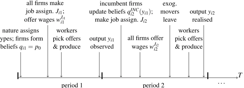
The timing of the events is the following. At the beginning of period 1, nature
moves first to assign an ability type to each worker and this ability type is time
in-variant. Firms make period-1 job assignments and wage offers conditional on their
prior beliefs’ about a worker being good. Workers choose the firm with the highest
wage offer to work at. At the end of period 1, incumbent firms privately observe
workers’ outputs. At the beginning of the next period, incumbent firms update their
beliefs about workers’ ability types and announce job assignment decisions for their
previous period’s employees. After outside firms observe these job assignment
de-cisions, all firms make wage offers simultaneously. Workers privately learn about
their job-switching types in this period and the exogenous movers depart. Workers
then choose the firm with the highest wage offer to work at. If there are
multi-ple firms offering the same highest wage, a worker chooses randomly among those
highest-wage-offer firms but stays with her previous period’s employer if her
pre-vious period’s employer is one of the highest-wage-offer firms. Production then
begins. At the end of period 2, workers’ outputs are privately observed by their
period 1 period 2 . . . T nature assigns
types; firms form beliefsqi1=p0
all firms make job assign.Ji1;
offer wageswJi1
i1
workers pick offers & produce
outputyi1
observed
incumbent firms update beliefsqINC
i2 (yi1);
make job assign. Ji2
all firms offer wageswJi2
i2 exog. movers leave workers pick offers & produce
outputyi2
[image:15.612.121.529.113.261.2]realised
Figure 1: Timing of the job-assignment-wage-offer game.
Firms’ strategies are sequences of job-assignment and wage-offer pairs. Letwitj
denote the wage offer to worker i in period t. Jit denotes the job assignment to
worker i in period t. In equilibrium, the incumbent firm anticipates that outside
firms’ behavior would be affected by its promotion decisions. The best response
is to match the wage offer from outside firms and extract the rent created by the
firm-specific human capital. Therefore, the equilibrium wage offer from the
incum-bent firm is equal to the wage offer from outside firms and there is no turnover in
equilibrium except for the exogenous movers. A firm’s strategy set is
n
Jit,witj
o
t, j=Jit ∈ {l,m},t∈ {1, . . . ,T}.
Figure 1 shows the sequences of beliefs, job assignments, and wage offers after
3
The Analysis
In this section, I begin the analysis with a brief discussion about the equilibrium job
assignment rules and wage offers when a worker’s type is perfectly known. I then
consider what happens given asymmetric information and discuss the relationship
between non-promotion, negative signals, and wage dynamics.
3.1
A Full-information model with T periods
Under full information, workers’ types are fully observed by all firms. Each firm’s
problem is to assign workers to the jobs that maximise the total discounted profit.
Firms solve different problems when assigning workers who have worked for them
in the previous period and those who have not. This is because firms can collect
firm-specific human capital from the old workers in the current period but they
have to train new workers.
Consider a firm’s problem when it assigns workers who were employed by the
firm in the previous period, i.e., when the firm makes job assignment decisions and
wage offers as an incumbent firm. LetΠtINC(θi)denote the incumbent firm’s profit
in periodt from employing a worker who has a probabilityθiof attaining the high
productive efficiency. Πl
t(θi)is the non-promotion profit andΠmt (θi)is the
promo-tion profit from employing this worker. ThenΠINCt (θi) =max
Πtl(θi),Πmt (θi) ,8
8Since there is no turnover in equilibrium for non-exogenous movers and the probability of
where
Πtl(θi) = (1+S)[θizlH+ (1−θi)zLl +f(t−1)]−witl +βΠtINC+1(θi), (3)
Πmt (θi) = (1+S) [θizmH+ (1−θi)zLm+f(t−1)]−witm+βΠINCt+1(θi). (4)
wtjis the equilibrium wage that an incumbent firm offers, which is equal to
out-side firms’ wage offer.9 In periodt, the incumbent firm chooses a job-assignment-wage-offer pair to maximise the total discounted profit given workers’ types. If
non-promotion is more profitable, the firm assigns the worker to the lower level
job. Otherwise, the firm assigns the worker to the upper-level job. Due to the
firm-specific human capital, an incumbent firm can potentially make positive profit by
retaining an old worker.
When a firm makes decisions as an outside firm, i.e., when it considers wage
bids for workers in other firms, its problem is characterised by a zero profit
condi-tion (due to free entry). Thus, the equilibrium wage in periodtis equal to a worker’s
current period’s productivity plus potential discounted future profits at an outside
firm,ΠtOU T+1 (θi), i.e.,
witj(θi) = [θizHj + (1−θi)z j
L+f(t−1)] +βΠtOU T+1 (θi),j∈ {l,m},θi∈ {θg,θr}. (5)
In the last period, since there are no future periods, a worker’s wage is equal
9The expressions in 3 and 4 describe equilibrium behavior. The original firms’ problem for this
to her productivity in period T. In periods before T, a period-t “outside” firm
would become an “incumbent” firm from period t+1 onward. This is because
from periodt+1 onward, a period-t outside firm starts to collect the firm-specific
human capital as a period-t incumbent firm does. Since a period-t outside firm has
the same information about a worker as a period-tincumbent firm does, the outside
firm’s expected future profit is equal to an incumbent firm’s expected future profit
from periodt+1, i.e.,ΠtINC+1(θi) =ΠtOU T+1 (θi) =Πt+1(θi). Thus, we can substitute
(5) into (3) and (4), and an incumbent’s job-assignment problem simplifies to
ΠtINC(θi) =S·{max
l,m
[θizlH+(1−θi)zlL,θizmH+(1−θi)zmL]+f(t−1)},θi∈ {θg,θr}.
Since a good worker has higher expected productivity on the upper-level job
and an ordinary worker has higher expected productivity on the lower level job,
the good worker should be assigned to the upper-level job and the ordinary worker
should be assigned to the lower level job in each period. Also, since workers of
the same type are ex ante identical, the equilibrium wages are only functions of
workers’ types, i.e., all good workers are paid the same wage in a certain period
while all ordinary workers are paid another. I thus omit the individual subscript in
the wage equations in the rest of this section.
I summarise the job assignment rules and equilibrium wages under full
infor-mation in the following proposition. All proofs are provided in the appendix.
Proposition 1. Suppose each worker’s type is fully observable. Then the job
as-signment rules and the equilibrium wages satisfy (i) and (ii):
paid wtm(θg) = [Egm+ f(t−1)] +βS[Egm+f(t)]in period 1≤t <T ; she is paid
wmT(g) =Egm+ f(T−1)in period T ;
(ii) An ordinary worker is assigned to the labourer level in every period and
is paid wlt(θr) = [Erl+ f(t−1)] +βS[Erl+ f(t)] in period1≤t <T ; she is paid
wliT(r) =Erl+f(T−1)in period T .
From Proposition 1, only the next period’s productivity matters for the
equi-librium wage. This is because the future profit is the extra economic rent that an
incumbent firm can extract from collecting the benefit of one more period of
firm-specific human capital compared to an outside firm. Thus, the rent is the next
period’s productivity multiplied by the firm-specific human capital factor S. This
rent gives an outside firm an incentive to become an incumbent firm in the next
period by bidding away a worker in the current period. Since firms are competing
with each other over workers, all the economic rent is reflected in the equilibrium
wage. The higher the firm-specific human capital is, the more a firm is willing
to pay in anticipation of a higher rent from collecting the firm-specific part of the
productivity.
Now let us consider how the timing of promotion is related to workers’ wages.
An ordinary worker’s wage growth on the labourer job between two periods is
wtl+1(r)−wtl(r) = [f(t)− f(t−1)] +βS[f(t+1)− f(t)] >0. That is, a non-promoted worker’s wage always increases with job tenure. A similar pattern is
observed for good workers’ wages. The reason is that under full information there
is no learning with additional tenure, so workers’ wages are determined solely by
human capital accumulation which is non-decreasing with additional tenure.
non-promoted workers’ wages first increase then decrease with tenure on the same job
level for workers who spend a long time on the same job level. In the next section,
I consider what happens when learning is asymmetric. I show that with
asymmet-ric learning, non-promotion interacts with human capital accumulation and affects
workers’ wage dynamics through learning.
3.2
A Model with Asymmetric Information
With asymmetric information, incumbent firms observe outputs and update their
be-liefs about a worker being good and then make job assignment decisions and wage
offers based on observed outputs. Outside firms observe workers’ job assignments
at the incumbent firms and update beliefs about workers’ ability types. I focus on
perfect Bayesian Equilibriums (PBE) of the model. That is, equilibrium beliefs are
derived based on Bayes’ rule given equilibrium strategies and equilibrium strategies
are optimal for the incumbent firms, the outside firms, and the workers given the
equilibrium beliefs.
Under the current framework, the incumbent firm never learns workers’ true
types. Furthermore, because of the binary output structure, when the incumbents
make promotion announcements, they convey their private information about a
worker’s output in the current period completely under the parameterizations
spec-ified in the previous section. That is, whenever an incumbent firm observes the
high-level productive efficiency, a worker is promoted; whenever an incumbent firm
observes the low-level productive efficiency, a worker stays on the same job level
(a promoted worker stays on the upper level job). In anticipating these
was attained at the labourer job when a promotion is observed; while a low-level
productive efficiency was attained if a non-promotion is observed. It remains to
check that under those beliefs the incumbents’ strategies are indeed optimal.
The firms’ problem is similar to the one under full information, i.e., incumbent
firms choose a job-assignment-wage-offer pair to maximise total expected profit.
The difference is that, since workers’ types are unknown, workers’ expected
pro-ductivity is determined by the belief that a worker is good. LetΠINCt (qINCit )denote
the incumbent firm’s profit in periodt from employing a worker who is believed
(by the incumbent firm) to be good with probability qINCit . Πtl(qINCit ) is the
non-promotion profit andΠmt (qINCit )is the promotion profit from employing this worker.
ThenΠINCt (qINCit ) =max
Πtl(qINCit ),Πtm(qINCit ) , where
Πlt(qINCit ) = (1+S)[qitINCEgl+ (1−qINCit )Erl+f(t−1)]−wlit+βΠINCt+1(qINCit ,l),
(6)
Πtm(qINCit ) = (1+S)[qINCit Egl+ (1−qINCit )Erl+f(t−1)]−wmit +βΠINCt+1(qINCit ,m).
(7)
ΠINCt+1(qINCit ,j),j ∈ {l,m}, is the incumbent’s future expected profit given the
belief int that a worker is good with probabilityqINCit and the fact that the worker
is assigned to job jin periodt.
The outside firms’ problem is characterised by a zero profit condition, so an
outside firm is willing to bid above a worker’s current period’s expected
productiv-ity because it can collect future rents when it becomes an incumbent firm. Similar
next period’s job assignment and productivity are relevant to the expected rents
because an incumbent firm only collects one more period of firm-specific human
capital compared to an outside firm.
Outside firms’ wage bids are
wlit(qOU Tit ) = [qOU Tit Egl+ (1−qOU Tit )Erl+f(t−1)] +βΠtOU T+1 (qOU Tit ,l), (8)
wmit(qOU Tit ) = [qOU Tit Egl+ (1−qOU Tit )Erl+f(t−1)] +βΠtOU T+1 (qOU Tit ,m), (9)
where qOU Tit denotes the outside firm’s belief in period t that worker i is good;
ΠtOU T+1 (qOU Tit ,j)denotes the outside firm’s future expected profit given the belief in
tthat a worker is good and the fact that the worker is assigned to job jin periodt.
Note that under asymmetric information, an outside firm’s belief that a worker is
good is based on the incumbents’ job assignment signals while the incumbent’s
be-lief is based on workers’ output realizations. That is, an incumbent firm and an
out-side firm have different information sets about each worker. Thus, the outout-side firm’s
belief about the worker and the expected future rents from this worker might be
dif-ferent from the incumbent firm’s. However, parameter restriction (ii) guarantees
that the incumbent firm promotes a worker when a high output is observed.
There-fore, at the time of promotion, the incumbent and the outside firms have the same
information about a non-promoted worker, i.e.,qINCit =qOU Tit =qit,ΠINCt+1(qINCit ,j) =
sim-plifies to
Πt[qit(hti−1)] =S· max
l,m
n
E[ylit|qit(hti−1)],E[ymit|qit(hti−1)]
o
=S· max
l,m
n
qit(hti−1)Egl+ [1−qit(hti−1)]Erl,qit(hti−1)E m
g + [1−qit(hti−1)]Erm
o
+S·f(t−1).
Therefore, the equilibrium strategy is that if the belief of a worker being good is
greater than the threshold, i.e.,qit≥q∗(recall thatq∗equates the expected
produc-tivity on the two job levels), the worker is promoted. Otherwise, the worker remains
in the previous job level. Given parameter restriction (i), once a high productive
ef-ficiency is observed (for the first time), the belief of this worker being good would
be above the threshold and thus this worker will be promoted by an incumbent
firm, i.e., sinceqit(1)>qiT(1)>q∗, once a worker attains the high productive
ef-ficiency, she is assigned to the manager position and remains there independent of
subsequent output realizations.
At an outside firm, given the observed job assignment history, the expected
future profit to an outside firm is the same whether the worker is assigned to the
manager position or the labourer position in the current period. Thus, an outside
firm only considers the current period’s expected output when deciding where to
as-sign a worker. If an outside firm observes a promotion (non-promotion), it believes
that this worker has produced high (low) output at the incumbent firm and thus she
a promoted (non-promoted) worker at an incumbent firm is also assigned to the
upper-level (lower-level) job at an outside firm.
LetEt[Zitj|qit(hti−1)]denote the part of the expected productivity int that is
de-termined by workers’ ability types given the observed information up tot−1, i.e.,
Et[Zitj|qit(hti−1)] =qit(hti−1)Egj+ [1−qit(hti−1)]Erj. LetEt[Zitj+1|qit(hti−1),j]denote
the part of the expected productivity int+1 from periodt’s perspective that is
de-termined by workers’ ability types given the observed information up tot−1 and
the job assignment in t. The expression for Et[ZitJit++11|qit(hti−1),j] is given in the
appendix.
I summarise the job assignment rules and equilibrium wages under asymmetric
information in the following proposition.
Proposition 2. Suppose workers’ types are not observed but the incumbent firms
can observe workers’ outputs and the outside firms can observe workers’ job
as-signments. Given the prior belief that a worker is good with probability p0, the job
assignment rules and the equilibrium wages satisfy (i) to (iv):
(i) All workers are assigned to the lower level job in period 1.
(ii) Let ti be the first period in which worker i produces the high output. Then
worker i is assigned to the labourer position in each period t,t≤ti. Her wage in t
is witl[qit(0)] ={Et[Zitl|qit(0)] + f(t−1)}+βS{Et[ZitJit++11|qit(0),l] +f(t)}.
(iii) Worker i is assigned to the manager position in each period t,ti+1≤
t <T . Her wage in t is wmit[qiti+1(1)] ={Et[Z
m
it|qiti+1(1)] + f(t−1)}+β{(1+
S)Et[ZitJit++11|qiti+1(1),m]−Et[Z
m
it|qiti+1(1)] +S f(t)}.
(iv) In period T , if ti≤T−1, the worker is assigned to the manager job and is
paid wmiT[qiti+1(1)] =E[Z
m
the labourer job and is paid wliT[qiT(0)] =E[ZiTl |qiT(0)] + f(T−1).
Note that for workers who have attained the high productive efficiency before
period T−1, outside firms’ beliefs about their types stop updating once they are
promoted because outside firms cannot infer their outputs from job assignments
anymore (see (iv in Proposition 2). However, outside firms expect a promoted
worker to produce either high or low in the next period because there is no
win-ner’s curse and incumbents do not observe workers’ types perfectly. After a worker
worked for a firm for one period, the firm starts to collect new information about
this worker. Thus, the expected rent derived from employing this worker is the
difference between the worker’s expected productivity at an incumbent firm in the
next period, (1+S){Et[ZJit+1
it+1|qiti+1(1),m] +f(t)}, and the worker’s expected
pro-ductivity at an outside firm in the next period,Et[Zitm|qiti+1(1)] +f(t).
Now, let us consider how the non-promotion wages change with job-tenure.
Note that all workers with the same output history are ex ante identical (i.e.,qit(0) =
qkt(0),i6=k). That is, all the non-promoted workers in periodt are paid the same
wage. In the following discussion, I omit the subscriptifor individuals. The wage
paid to a worker who is on level l for t periods ( i.e. she has attained the
low-level productive efficiency in the previoust−1 periods) thus is wtl[qt(0)], and the
wage paid to a worker who is on levell fort+1 periods ( i.e. she has attained the
low-level of productive efficiency in the previoustperiods), iswlt+1[qt+1(0)].
Corollary 1. Under asymmetric information, there exists a t1∗,2<t1∗≤t, such that¯
if the following conditions are satisfied, the non-promoted workers’ wages increase
wlt[qt(0)]<wlt+1[qt+1(0)]; for t >t1∗+1, wtl[qt(0)]>wtl+1[qt+1(0)]if
f(t1∗+1)− f(t1∗)>[q2(1)−q3(1)][Egl−Erl], and (10)
f(t1∗+2)−f(t1∗+1)<[qt¯(1)−qt¯+1(1)][Egl−Erl].10 (11)
Corollary 1 says that when human capital accumulation exceeds the negative
learning about workers’ ability with additional tenure, wages increase; when
hu-man capital grows little between two periods, the negative learning about workers’
abilities lead to a wage decrease.
To see how the conditions in (10) and (11) guarantee the wage patterns
de-scribed in Corollary 1, note that as additional low outputs are observed, the
ex-pectation that a worker is good decreases, i.e., qt(0)>qt+1(0), fort ≥2. Since
Egl >Erl, the part of the wage that is related to workers’ ability types,Et[Ztl|qt(0)] =
qt(0)Egl+ [1−qt(0)]Erl, decreases when firms put a smaller weight on the belief
that a worker is good. Similarly, the forward expectation,Et[ZtJ+t+11|qt(0),l], also
de-creases int, because it is less likely that a worker would produce high in the next
period if she has produced more low outputs in the past. Since both expectations are
bounded, if there is substantial human capital accumulation from periodt to period
t+1, the non-promotion wage increases. If the human capital accumulation from
periodtto periodt+1 is sufficiently small, the non-promotion wage decreases. By
construction, since human capital accumulates very fast whent approaches 1 and it
almost stops growing after ¯t, there exists at least one period between period 2 (note
that tenure in period 2 is equal to 1) and period ¯t+1 such that the non-promotion
Furthermore, the expectation about workers’ types decreases at a decreasing
speed and eventually approaches zero whent approaches∞. Thus, the largest
de-crease in expectation is between period 2 and 3. On the other hand, human
cap-ital increases at a decreasing speed and eventually approaches zero when t
ap-proaches ¯t <∞. Thus, the largest increase in human capital after period t1∗+1 is f(t1∗+2)− f(t1∗+1). The condition in (10) guarantees that in periods before
t1∗+1 the smallest human capital accumulation outweighs the largest expectation decrease. Thus, workers’ wages increase before periodt1∗+1. After that, the condi-tion in (11) guarantees that the largest human capital accumulacondi-tion is smaller than
the smallest expectation decrease. Therefore, workers’ wages decrease after period
t1∗+1.11
As graphed in Baker et al. (1994a), for workers who are promoted from level 1
to level 2 within six years of tenure on level 1, their (real) wages prior to the
pro-motion increase with each additional year of job-level tenure. For workers who are
promoted after the sixth year, their wages prior to the promotion first increase then
decrease with additional level-1 tenure. This empirical finding departs from
Bern-hardt’s (1995) prediction that the non-promotion wages either increase or decrease
monotonically with firm-level tenure but is captured in the above Corollary.
Using a similar argument, one can examine the wage-tenure relation for wages
upon promotion.
Corollary 2. Under asymmetric information, there exists a t2∗,3<t2∗≤t, such that¯
if the following conditions are satisfied, the promotion wages increase in periods
11If the conditions in (10) and (11) are not satisfied, I still get the result that non-promoted
before t2∗+1and decrease in periods after t2∗+1, i.e., for3≤t<t2∗+1, wtm[qt(1)]<
wmt+1[qt+1(1)]; for t >t2∗+1, wtm[qt(1)]>wmt+1[qt+1(1)]if
f(t2∗+1)−f(t2∗)> 1+S
S [q4(2)−q5(2)][E
l
g−Erl], and (12)
f(t2∗+2)−f(t2∗+1)<(1−β)[qt¯(2)−qt¯+1(2)][Egl−Erl]. (13)
Similar to the non-promotion wage, the wage in the period of promotion first
increases then decreases with more time spent on the lower level job before
promo-tion. Baker et al. (1994a) find that if a worker earns a promotion within four years
on level 1, the wage that she earns upon promotion is higher than the wage paid to
someone who is promoted in the previous period. On the other hand, if a worker
earns a promotion after spending more than four years on level 1, the wage that she
earns upon promotion is lower than the wage paid to someone who is promoted in
the previous period.
Note that the condition in (12) is stronger than that in (10) sinceqt(2)−qt+1(2)>
qt(1)−qt+1(2)>qt(0)−qt+1(0). Therefore, it is possible thatt2∗<t1∗, which means
the promotion wage falls before the non-promotion wage does.
It is worth noticing that the signaling effect is embedded in job-tenure rather
than firm-tenure. In the current set up, the level-l job-tenure is equal to firm-tenure
before promotion. Suppose I were to extend the model to include a level below
the labourer’s level, call it the routine level, where workers’ productivities do not
vary with abilities and workers in this level are randomly selected into the labourer’s
level. If we compare a worker who has eleven years of firm tenure with four years on
of firm-tenure with two years on the routine job and eight years on the labourer’s
job, if both workers are not promoted in the current period, the former would earn
a higher wage than the latter although she has longer firm-tenure. The latter has a
lower wage because she spends more time on the labourer’s position. That is, the
negative signal is associated with job-tenure rather than firm-tenure.
4
Data and Tests
In Baker et al. (1994a), the wage-job-tenure profile is shown using a raw plot. In
this section, I use the same dataset that they have studied to estimate a tenure-wage
equation controlling for other observables. I focus on the relationship between
job-tenure and non-promotion wages as well as the relationship between job-job-tenure
(before promotion) and promotion wages.
The dataset was constructed by George Baker, Michael Gibbs, and Bengt
Holm-strom from the personnel records of a medium-sized US firm in the financial
ser-vices industry. It contains detailed information on workers’ demographic
charac-teristics, tenure, subjective performance evaluation, and promotion history. In their
seminal papers, Baker et al. (1994a;b) provide a thorough analysis of wage and
ca-reer dynamics in this firm during a 20-year period from 1969 to 1988 using the full
sample of managerial employees for a total of 68,437 employee-year data points.
In this analysis, I restrict the sample to US white males to focus on the wage
dy-namics without concerning the gender-wage-gap. I also exclude demotion, which
takes up 2%-3% of the sample. Since I use a one-year lag in calculating job-tenure,
per-Table 1: Levels, Titles, and Education
Level TITLE HS BS MA PHD Total
1 AH 80 78 16 7 181
N=4,699 44.2 43.09 8.84 3.87 100 Pct.=29.63% AJ 1,460 1,301 481 31 3,273 44.61 39.75 14.7 0.95 100
AK 766 402 77 0 1,245
61.53 32.29 6.18 0 100
2 H 59 73 20 17 169
N=5,399 34.91 43.2 11.83 10.06 100
Pct.=34.05% I 43 124 21 0 188
22.87 65.96 11.17 0 100
J 97 134 70 17 318
30.5 42.14 22.01 5.35 100
K 428 180 59 0 667
64.17 26.99 8.85 0 100 L 1,406 585 209 3 2,203 63.82 26.55 9.49 0.14 100 M 551 848 409 46 1,854 29.72 45.74 22.06 2.48 100
3 F 21 80 22 0 123
N=5,759 17.07 65.04 17.89 0 100 Pct.=36.32% G 2,327 1,905 1,056 105 5,393 43.15 35.32 19.58 1.95 100
SH 47 148 24 24 243
[image:30.612.146.466.205.606.2]formance measure and I exclude years of schooling 15,17,19, and 20 since those
years of schooling are hard to categorise with a degree measure. There are eight job
levels, where level 8 is the CEO position.12 I only look at workers on levels 1 to 3 since the promotion and wage dynamics on upper-level jobs might be very different
from those on lower level jobs. Moreover, I want to focus my analysis on the same
sample that generates the wage plots in Baker et al. (1994a). In those plots, they
focus on the wage and job-tenure relations on level 1 through level 3. This sample
selection procedure gives me a sample of 15,857 employee-year data points across
three job levels.
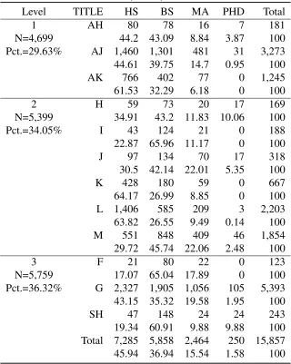
Table 1 presents the 17 major job titles as specified in Baker et al. (1994a;b),
grouped by job levels and interacted with education groups following DeVaro and
Waldman (2012). Observations are roughly equally distributed across three job
levels, with 30% from level 1, 34% from level 2, and 36% from level 3. There are
12 job titles on level 1 to 3 but there are one or two job titles that are the dominant
job title on a particular level.
Table 2 presents the descriptive statistics. Supervisor subjective performance
ratings are measured annually on a five-point scale where 1 denotes the best
perfor-mance and 5 the worst. There are roughly equal numbers of employee-years in the
three job levels. The average tenure at the firm is 3.7 years and the average tenure
in the job level is 2.6 years. Workers on average spend 2.3 years on level 1 before
being promoted to level 2. They spend a little longer, 2.6 years, on level 2 before
being promoted to level 3. Around 15% of the employees are promoted in each
sample year.
Table 2: Summary Statistics
Variable Obs Mean Std. Dev. Min Max Real Salary (in 1988 dollar) 15857 46726.37 10483.57 20846.91 109890.10
∆Real Salary 11859 1644.12 3047.10 -13522.83 30163.46
∆% Real Salary 11859 0.04 0.07 -0.24 0.91 Age 15857 39.03 9.43 23.00 69.00 High School 15857 0.46 0.50 0.00 1.00 Bachelor 15857 0.37 0.48 0.00 1.00 Master 15857 0.16 0.36 0.00 1.00
PhD 15857 0.02 0.12 0.00 1.00
Performance Rating (t-1) 11859 1.95 0.71 1.00 5.00 Year at Company (t-1) 13372 3.74 3.51 0.00 18.00 Year at Level (t-1) 15086 2.60 2.56 0.00 17.00 Promotion 15857 0.15 0.36 0.00 1.00
To test the job-tenure-wage profile, I consider the following wage equation.
wit =β0+β1Lit−1+β2Wi0+β3Xit−1+εit (14)
iindexes an individual andt indexes years. Xit−1is a vector of controls
includ-ing age and age squared, education, and performance ratinclud-ing in the previous year.
Lit−1is year at level int−1 before promotion. Thus, it denotes the job-level tenure
at the previous level for a just promoted worker and job-level tenure at the current
level up tot−1 for a non-promoted worker.Wi0is workeri’s first salary at the firm,
which is a control for workers’ initial characteristics (Belzil et al., 2012).
Work-ers’ initial characteristics need to be controlled for because the model predictions
concern learning about ex ante identical workers. Since the initial wage carries rich
information about an individual, I use it as a proxy for workers’ initial
heterogene-ity.
re-Table 3: Wage-tenure profile before promotion (quadratic): level=1
(1) OLS (2) OLS (3) OLS (4) OLS (5) FE
Dependent Variable: Real Salary in 88 Dollars
Yr. at Level 80.128 1,120.291** 771.463** 1,256.270** 1,002.114** (t-1) (53.370) (111.222) (124.559) (214.247) (127.373) Yr at Level2 -135.559** -99.508** -112.916** -79.256** (t-1) (12.083) (12.466) (17.230) (10.237) Entry Salary 0.328** 0.328** 0.313** 0.353**
(0.014) (0.014) (0.014) (0.024)
Rating (t-1) -2,333.563**
(244.979)
Age (t-1) 1,170.840** 889.369** 1,905.166**
(87.675) (137.627) (254.780)
Age2(t-1) -14.225** -11.218** -24.356**
(1.071) (1.593) (2.885)
High School -307.858 -827.032*
(250.931) (354.364)
Master 3,649.813** 2,721.757**
(349.193) (612.507)
PhD 2,863.510** 1,972.203
(890.531) (1,145.488)
Constant 31,559.206** 30,848.928** 8,778.494** 18,337.007** 3,235.066 (341.818) (346.468) (1,642.439) (2,709.431) (5,608.402)
Observations 4,516 4,516 4,516 2,338 4,518
R-squared 0.147 0.166 0.223 0.237 0.954
[image:33.612.110.560.212.572.2]stricted to those individuals who are on the same job level in a particular year and
I consider individuals on different job levels separately. The sample that I use to
test the promotion-wage-job-tenure relation is restricted to those individuals who
are just promoted in a particular year and I consider the individuals who are
pro-moted from level 1 to level 2 and those who are propro-moted from level 2 to level 3
separately.
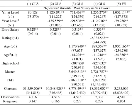
Table 3 looks at the relationship between job-tenure and non-promotion wages
(in real terms) for those individuals on level 1. The table begins with the most
par-simonious specification with only job-tenure in the previous period and the entry
salary as the explanatory variables in Column (1). There is a positive relationship
between wage and job-tenure but it is not statistically significant. Each column
from (2) to (4) adds additional controls. Column (2) adds a quadratic term for
job-tenure. Column (3) includes controls for age and education. Column (4) adds
con-trols for performance rating. The hump-shaped wage-job-tenure relation remains
after I control for performance rating. However, in the theoretical model workers’
wages are not conditioned on their output, which can be reflected in the
perfor-mance measure, so column (3) is a better test of the theory without controlling for
the performance rating.13 In Column (5), I consider a fixed-effect model on in-dividual level excluding performance ratings. The relationship between job-tenure
and the non-promoted workers’ wage persists regardless of model specifications. In
particular, the non-promoted workers’ wage first increases then starts to fall. These
results match Baker et al.’s (1994a) wage plots very well.
Note that, the OLS models compare the average wages across individuals and
13See DeVaro and Waldman (2012) for a discussion of using performance rating as a measure of
the fixed-effect model captures within person wage dynamics. From the
theoreti-cal model, all the non-promoted workers in a given period are paid the same wage
because they are identical in all other dimensions. In practice, workers differ in
age, education, performances and other dimensions. Therefore, I control for other
observables in the OLS models. However, there might still be other unobserved
individual characteristics that are driving the results. So the estimates of the OLS
models capture two effects. First, those individuals who stay on level 1 for a shorter
period of time on average earn a higher wage than those who stay longer because
the former are more able to earn a promotion earlier. Second, each individual has
a smaller wage increase (and eventually wage decrease) with longer tenure on the
same level. The theoretical model suggests that we should also observe the
hump-shaped wage-tenure pattern when we compare within individuals and these
predic-tions are supported by the estimates from the fixed-effect model.14
Table 4 examines the job-tenure-non-promotion-wage relation using job-tenure
dummies instead of imposing the quadratic form on job-tenure in the wage
equa-tion. We can see that the non-promoted workers’ wages increase with job-tenure
then start to fall after four or five years. For example, from Column (1), with three
year tenure on job 1, a worker’s wage is $1,969 higher than the entry wage; with
four year tenure on job 1, a worker’s wage is only $1,544 higher than the entry
wage, which means the worker’s wage starts to fall in the fourth year. If a worker
spends more than six years on level 1 without a promotion, her wage even falls
be-14There is a discrepancy between the theory and the empirical specification in (14) that in the
Table 4: Wage-tenure profile before promotion (year dummies): level=1 (1) OLS (2) OLS (3) OLS (4) FE Yr at Level(t-1) Dependent Variable: Real Salary in 88 Dollars
1 1,327.494** 850.815** -677.111 1,193.591** (289.458) (286.645) (353.374) (141.784) 2 1,603.746** 784.368* 407.647 2,138.382**
(357.945) (377.822) (344.477) (223.858) 3 1,969.184** 1,010.640* 800.016 2,845.665**
(470.574) (500.490) (457.721) (328.424) 4 1,544.368** 530.355 526.257 3,057.691**
(544.806) (569.671) (535.426) (388.907) 5 716.288 -267.627 188.531 3,398.000**
(643.595) (660.488) (626.804) (494.805) 6 -325.991 -1,109.076 -127.689 3,224.353**
(780.660) (813.315) (753.214) (601.316) 7 -944.832 -1,641.365 -850.610 3,142.963**
(989.624) (977.187) (922.020) (755.284) 8 -4,072.561** -4,371.377** -3,399.209** 2,132.144*
(1,096.801) (1,089.629) (1,072.734) (877.605) 9 -4,696.114** -5,248.299** -4,232.494** 2,884.836**
(1,485.813) (1,480.712) (1,419.875) (1,084.924) 10 -6,822.486** -6,992.827** -5,512.765** 3,278.206* (1,876.262) (1,573.646) (1,565.759) (1,424.512) 11 -4,745.591 -5,859.753* -4,843.347 2,259.449
(3,485.411) (2,812.724) (2,894.402) (1,975.629) 12 -6,727.453** -6,466.210** -5,047.442** 1,521.800
(807.280) (1,284.532) (1,300.991) (1,391.815) 13 -7,321.807** -6,495.907** -5,126.091** 1,897.945
(913.263) (1,207.943) (1,206.696) (1,656.205) Entry Salary 0.327** 0.313** 0.354** No
(0.014) (0.014) (0.024) No
Age No Yes Yes Yes
Education No Yes Yes No
Rating No No Yes No
Constant 38,402.605** 13,989.254** 24,168.928** 7,151.725 (175.917) (1,729.504) (3,103.598) (5,009.659) Observations 4,518 4,518 2,338 4,518
R-squared 0.026 0.097 0.107 0.954
low the entry level. These patterns remain after I control for age and education in
Column (2). In Column (3), I add controls for performance rating. The wage pattern
remains. Column (4) presents the fixed-effect estimates with job-tenure dummies.
We can see that workers wages increase fast in the first five years on the job and
[image:37.612.111.566.253.612.2]starts to fall in the sixth year.
Table 5: Wage-tenure profile before promotion(quadratic): level=2
(1) OLS (2) OLS (3) OLS (4) OLS (5) FE
Dependent Variable: Real Salary in 88 Dollars
Yr. at Level -20.267 1,084.606** 733.951** 913.175** 454.667** (t-1) (34.432) (128.834) (146.204) (166.053) (88.055) Yr at Level2 -88.054** -59.899** -46.615** -50.066**
(t-1) (9.830) (10.967) (13.778) (6.686)
Entry Salary 0.308** 0.338** 0.317** 0.373** (0.013) (0.013) (0.013) (0.016)
Rating (t-1) -2,361.349**
(181.537)
Age (t-1) 1,179.609** 1,117.072** 2,388.337** (91.296) (101.540) (220.122)
Age2(t-1) -13.988** -13.186** -25.694**
(1.078) (1.179) (2.488)
High School -801.273** -791.539**
(265.289) (283.761)
Master 3,055.688** 2,475.624**
(342.154) (378.475)
PhD 1,960.592* 1,313.417
(944.297) (1,115.009)
Constant 37,490.788** 35,143.455** 12,620.226** 16,757.512** -7,025.540 (317.198) (425.766) (1,764.041) (1,980.936) (4,636.120)
Observations 4,574 4,574 4,574 3,779 5,141
R-squared 0.111 0.127 0.174 0.199 0.930
Robust standard errors in parentheses ** p<0.01, * p<0.05
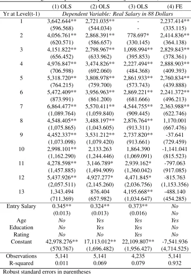
Table 6: Wage-tenure profile before promotion(year dummies): level=2 (1) OLS (2) OLS (3) OLS (4) FE Yr at Level(t-1) Dependent Variable: Real Salary in 88 Dollars
1 3,642.644** 2,721.035** - 2,237.414** (596.568) (544.034) - (335.115) 2 4,056.761** 2,868.391** 778.697* 2,414.836**
(620.571) (586.657) (330.145) (364.138) 3 4,151.822** 2,798.967** 1,098.994** 2,829.843**
(656.452) (633.962) (395.853) (378.361) 4 4,976.847** 3,474.826** 2,227.494** 2,888.903**
(706.598) (692.060) (484.368) (409.393) 5 5,318.720** 3,808.978** 2,861.933** 2,760.834**
(764.215) (759.700) (573.743) (439.888) 6 5,472.409** 3,956.963** 2,869.221** 2,241.372**
(873.991) (861.200) (681.666) (496.213) 7 6,864.477** 5,570.411** 4,544.755** 2,363.988**
(1,089.764) (1,059.840) (909.445) (622.746) 8 4,548.405** 3,488.197** 2,876.764** 1,170.001 (1,075.865) (1,043.605) (913.311) (667.476) 9 4,452.337** 3,531.212** 2,737.820** -37.641
(1,073.098) (1,079.420) (913.661) (729.459) 10 2,998.101** 2,133.263 1,864.390 -1,141.041
(1,162.290) (1,244.446) (1,069.091) (815.523) 11 4,278.598** 3,146.789* 2,939.162* -797.063
(1,457.885) (1,494.909) (1,360.042) (917.085) 12 5,437.926** 4,927.277* 4,471.845* -815.763
(2,057.511) (2,145.260) (2,036.756) (1,153.356) 13 1,343.494 876.404 4,195.668** -488.140
(711.369) (657.982) (1,034.647) (454.285) Entry Salary 0.345** 0.324** 0.373** No
(0.013) (0.013) (0.016) No
Age No Yes Yes Yes
Education No Yes Yes No
Rating No No Yes No
Constant 42,978.276** 17,113.012** 22,109.807** -7,541.936 (570.767) (1,696.482) (1,956.427) (4,714.525) Observations 5,141 5,141 4,235 5,141
R-squared 0.011 0.069 0.079 0.932
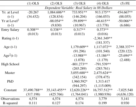
stay on level 2. The hump-shape wage-tenure profile is still evident in both
speci-fications with either a quadratic term on year-at-level or job-tenure dummies.
Col-umn (4) in each table controls for age, education and performance rating. ColCol-umn
(5) considers a fixed-effect model. From the fixed-effect model, the non-promotion
wage on level 2 starts to fall in year 5.
Note that I do not control for firm tenure for the non-promoted workers for two
reasons. First, for individuals who are on level 1, their firm tenure is equal to their
job tenure. Second, for a non-promoted worker on level 2, conditional on firm
tenure, those who have longer 2 tenure in general should have shorter
level-1 tenure. If more able workers are promoted earlier on level level-1, those individuals
who have longer level-2 tenure should earn a higher wage. On the other hand, long
tenure on level 2 sends a negative signal. So, holding firm tenure fixed, the theory
predicts that wages can either increase or decrease with job tenure on level 2. The
current specification without controlling for firm tenure examines the average effect
of level-2 tenure on wages allowing individuals to have different years of tenure on
level 1.
Table 7 examines the average wages in the year of promotion for workers with
different job-tenure on the lower level job before promotion. Columns (1) and (2)
consider the promotion wage when a worker is promoted from level 1 to level 2.
From Column (1), the promotion wage first increases then decreases with tenure
on the job before promotion but the estimates are not statistically significant. From
Column (2), the promotion wage increases when tenure on the previous job is low
and decreases with tenure on the previous job is high but the relationship flips signs