Munich Personal RePEc Archive
Exponential Smoothing, Long Memory
and Volatility Prediction
Proietti, Tommaso
Dipartimento di Economia e Finanza
10 July 2014
Exponential Smoothing, Long Memory and Volatility
Prediction
Tommaso Proietti
Department of Economics and Finance, University of Rome Tor Vergata, Italy,
and CREATES, Aahrus University, Denmark
Abstract
Extracting and forecasting the volatility of financial markets is an important empirical problem. Time series of realized volatility or other volatility proxies, such as squared returns,
display long range dependence. Exponential smoothing (ES) is a very popular and successful forecasting and signal extraction scheme, but it can be suboptimal for long memory time series.
This paper discusses possible long memory extensions of ES and finally implements a general-ization based on a fractional equal root integrated moving average (FerIMA) model, proposed originally by Hosking in his seminal 1981 article on fractional differencing. We provide a
decomposition of the process into the sum of fractional noise processes with decreasing orders of integration, encompassing simple and double exponential smoothing, and introduce a low-pass real time filter arising in the long memory case. Signal extraction and prediction depend
on two parameters: the memory (fractional integration) parameter and a mean reversion pa-rameter. They can be estimated by pseudo maximum likelihood in the frequency domain. We
then address the prediction of volatility by a FerIMA model and carry out a recursive forecast-ing experiment, which proves that the proposed generalized exponential smoothforecast-ing predictor improves significantly upon commonly used methods for forecasting realized volatility.
Keywords: Realized Volatility. Signal Extraction. Permanent-Transitory Decomposition.
1
Introduction
Volatility is an important characteristic of financial markets. Its measurement and prediction has attracted a lot of interest, being quintessential to the assessment of market risk and the pricing of financial products. A possible approach is to adopt a conditionally heteroscedastic or a stochastic volatility model for asset returns, see Engle (1995) and Shephard (2005) for a collection of key references in these areas. Alternatively, we can provide a statistical model for a time series proxy of volatility, such as daily realized volatility measures, see e.g. McAleer and Medeiros (2008), or squared returns (possibly after a logarithmic transformation of the series). This paper is based on the latter approach and takes as well established fact the presence of long range dependence as a characteristic feature of volatility, see Ding, Granger and Engle (1993), Bollerslev and Wright (2000), Taylor (2005, section 12.9), Andersen et al. (2001), Hurvich and Ray (2003), among oth-ers, though this point is not without controversy (see, e.g. Diebold and Inoue, 2001, and Granger and Hyung, 2004, who illustrate that stochastic regime switching and occasional breaks can mimic long range dependence).
Long memory is often modelled by a parametric model featuring fractional integration. Letting
{yt}denote a univariate random process andB the backshift operator,Bkyt=yt−k, a basic model
(Granger and Joyeux, 1980, and Hosking, 1981) is the fractional differenced noise,
(1−B)dyt=ξt, ξt∼WN(0, σ2),
where d is the memory parameter, WN(0, σ2) denotes white noise, a sequence of uncorrelated
random variables with zero mean and variance σ2, and, for non-integer d > −1, the fractional
differencing operator is defined according to the binomial expansion as
(1−B)d=
∞
X
j=0
Γ(j−d) Γ(j + 1)Γ(−d)B
j,
where Γ(·) is the gamma function. We shall denote this by yt ∼ FN(d). For d ∈ (0,0.5) the
process is stationary and its properties can be characterised by the autocorrelation function, which decays hyperbolically to zero, and its spectral density, which is unbounded at the origin. The model can be extended so thatξt is replaced by a stationary short memory autoregressive moving
aver-age (ARMA), leading to the important class of ARFIMA (autoregressive, fractionally integrated, moving average) processes. For comprehensive treatments of long memory time series see Palma (2007), Giraitis, Koul and Surgailis (2012) and Beran et al. (2013).
according to Granger’s (1980) seminal result, a long memory process can result from the con-temporaneous aggregation of infinite first order AR processes). The heterogeneous autoregressive model (HAR) model by Corsi, based on a constrained long autoregressive model depending only on three parameters, associated to volatility components over different horizons (daily, weekly and monthly), can mimic the long memory feature and has proved extremely practical and successful in predicting realized volatility.
At the same time, there is growing interest in decomposing volatility into its short and long run components. Engle and Lee (1999) introduced a component GARCH model such that the conditional variance is the sum of two AR processes. Adrian and Rosenberg (2008) formulate a log-additive model of volatility where the long run component, a persistent AR(1) process with non-zero mean, is related to business cycle conditions, and the short run component, a zero mean AR(1), is related to the tightness of financial conditions. Engle, Ghysels and Sohn (2013) have recently introduced multiplicative and log-additive GARCH-MIDAS model, where the long run component is a weighted average of past realized volatilities, where the weights follow a beta dis-tribution. Colacito, Engle and Ghysels (2011) formulate a multivariate GARCH-MIDAS compo-nent model for dynamic correlations. Related recent papers in the multivariate framework dealing with volatility components are Hafner and Linton (2010), Bauwens, Hafner and Pierret (2013), and Amado and Ter¨asvirta (2013, 2014).
Exponential smoothing (ES) is a very popular and successful forecasting scheme among prac-titioners, as well as a filter for extracting the long run component or underlying level of a time series; it has also been extensively applied to forecasting volatility and value at risk. Its success is not only due to its simplicity, but also for constituting a remarkably close approximation to the volatility extracted by popular parametric methods such as GARCH models, when asset returns are modelled. It has thus become a reference and it has been incorporated in the widely popular RiskMetrics methodology. However, it is inadequate for handling long memory in volatility, which is an important feature of realized volatility series and other volatility proxies, such as squared or absolute returns. ES is a linear filter with weights declining according to a geometric progression with given ratio, usually fixed at 0.94, as advocated by Riskmetrics (see RiskMetrics Group, 1996). For long memory time series Riskmetrics (see Zumbach, 2007) has proposed a new methodology, referred to as RM2006, which aims at mimicking a filter with weighs decaying at a hyperbolic, rather than geometric, rate, by combining several ES filters with different smoothing constants.
(Fer-IMA) model, originally proposed by Hosking (1981): in the closing of his seminal paper, Hosking mentions two fractionally integrated processes that can prove useful in applications: the first is the generalized fractional Gegenbauer process, see Gray, Woodward and Zhang (1989), which has found many applications in the modelling of stationary stochastic cycles with long range depen-dence. The second is the FerIMA process (to be introduced in a later section), which according to Hosking (p. 175, last paragraph) “as a forecasting model it corresponds to fractional order multi-ple exponential smoothing”. The FerIMA process is a particular case of a fractional power process which has the representation (1−B)dy
t =
θ(B)
φ(B)
d
ξt, where φ(B) = 1−φ1B − · · · −φpBp,
andθ(B) = 1−θ1B− · · · −θqBq are polynomials in the lag operatorB with roots outside the
unit circle. To the author’s knowledge not much work has been done in this area, although there is some related work by Pillai, Shitan and Peiris (2012) and the class of Spectral ARMA models considered in Proietti and Luati (2014).
In the sequel we explore the characteristics of this process and propose a decomposition and corresponding filters that can be viewed as a generalization of exponential smoothing for fraction-ally integrated time series. The main result is the decomposition of a process integrated of order
d > 0into the sum of fractional noise processes of decreasing ordersd, d−1,d−2, etc. plus a stationary remainder term. The first component generalizes the ES filter to any value of the frac-tional differencing parameterd and has the following features: (i) it encompasses the traditional ES filter, as well as double exponential smoothing, when the order of integration is 2. (ii) In the long memory case the filter weights have a interesting analytic form, resulting from the multipli-cation of coefficients decaying at a geometric rate (as in traditional ES) and correction factors that decline hyperbolically. (iii) For a FerIMA process it yields a fractional noise process with the same integration order. (iv) It captures the persistent (long-run ifd >1) behaviour of the series as it can be characterised as a low-pass filter.
We address the issue of the empirical relevance of the volatility predictor arising from the Fer-IMA model by performing a recursive forecasting experiment and documenting that it almost systematically outperforms the RiskMetrics predictor as well as th HAC model.
case of a generalized Beveridge and Nelson (1981) decomposition, whereas section 6 analyses the properties of the FES filter as a low-pass filter in the frequency domain. In section 7 we briefly dis-cuss maximum likelihood estimation of the parameters of the FerIMA model and prediction. Our empirical assessment of the FerIMA predictor and signal extraction filter is presented in section 8. Section 9 concludes the paper.
2
Exponential smoothing
Letytdenote a time series stretching back to the indefinite past. The method known as exponential
smoothing (ES) yields thel-steps-ahead predictor ofyt,l = 1,2, . . .,
˜
yt+l|t=λ ∞
X
j=0
(1−λ)jyt−j. (1)
The predictor depends on the smoothing constant, λ, which takes vales in the range (0,1). The above expression is an exponentially weighted moving average (EWMA) of the available obser-vations. The weights received by past observations decline according to a geometric progres-sion with ratio1−λ. The eventual forecast function is a horizontal straight line drawn aty˜t+1|t.
The predictor is efficiently computed using either one of the two following equivalent recursions (adaptive-expectations formulae) :
˜
yt+1|t=λyt+ (1−λ)˜yt|t−1, y˜t+1|t = ˜yt|t−1 +λ(yt−y˜t|t−1). (2)
If a finite realisation is available,{yt, t = 1,2, . . . n}, and we denote byy˜1|0 the initial value of
(2), then
˜
yt+l|t =λ t−1
X
j=0
(1−λ)jyt−j+ (1−λ)ty˜1|0. (3)
If y˜1|0 = y1 (in which case y˜2|1 = y1), the weight of the first observation is increased, yielding
˜
yt+l|t = λPt−j=02(1− λ)jyt−j + (1− λ)t−1y1, and the weights attached to the past and current
observations sum up to unity. Alternatively, we could start the recursion with the average of the first
tobservations,y˜1|0 =Pjt−=01yt−j/t. The same solution is obtained by settingy˜1|0 = 0and rescaling
the weights so that they sum to one:y˜t+l|t= (1−(1−λ)t−1)−1λPt−j=01(1−λ)jyt−j. Comprehensive
reviews of exponential smoothing and its extensions are provided by Gardner (1985), Gardner (2006) and Hyndman et al. (2008).
It is well known that the ES predictor is the best linear predictor for the integrated moving average (IMA) process
whereB is the backshift operator,0 < θ < 1is the moving average parameter, and WN denotes white noise, a sequence of uncorrelated random variables with zero mean and variance σ2. In
particular
˜
yt+l|t =yt−θξt=
1−θ
1−θByt, (5)
is the minimum mean square predictor ofyt+lbased on the time series{yj, j ≤t}. This is
equiva-lent to the above EWMA withλ= 1−θ. The IMA(1,1) process admits the decomposition, known as the Beveridge and Nelson (1981) decomposition, into a permanent componentmt, represented
by a random walk (RW) process,mt=mt−1+ (1−θ)ξt, and a transitory purely random
compo-nent,et=θξt, so thatyt=mt+et. The permanent component is equal to the long run prediction
of the series at timetand it is thus measurable at timetbymt= (1−θ)(1−θB)−1yt.
A remarkable feature of the IMA(1,1) process and the associated ES forecasting scheme is that the one-step-ahead forecast is coincident with the long-run (eventual) forecast. This feature is only possessed by this model (which encompasses the RW).
The ES predictor is useful also in the presence of model misspecification: see Cox (1961) and Tiao and Xu (1993). Thus, it has potential also for a long memory process, if the parameterθ is estimated so as to minimise the multistep prediction error variance.
3
Riskmetrics 2006
Exponential smoothing has been used for forecasting and extracting the level of volatility from either squared returns or realized volatility measures according to the RiskMetrics methodology developed by J.P. Morgan. The Riskmetrics 1994 methodology (RM1994, see RiskMetrics Group, 1996) is based on a single EWMA with parameterλ= 0.06, or, equivalently,θ= 0.94.
The new RM methodology, referred to as RM2006 (see Zumbach, 2007), extends the 1994 methodology to the long memory case, by computing the one-step-ahead volatility prediction, denotedy˜t+1|t, as a weighted sum ofK exponentially weighted moving averages with smoothing
constantsλk, k = 1, . . . , K:
˜
yt+1|t = K
X
k=1
wky˜(t+1k)|t, y˜t(+1k)|t =λkyt+ (1−λk)˜yt(+1k)|t.
The weights decay according to
wk ∝1−
lnτk
lnτ0
,
whereτk, k = 0,1, . . . , K,are time horizons, chosen according to the geometric sequence:
τk =τ1ρk−1, k = 2, . . . , K, τ0 = 1560, τ1 = 4, ρ= √
The smoothing constants are related to the time horizons via
λk= 1−exp(−τk−1).
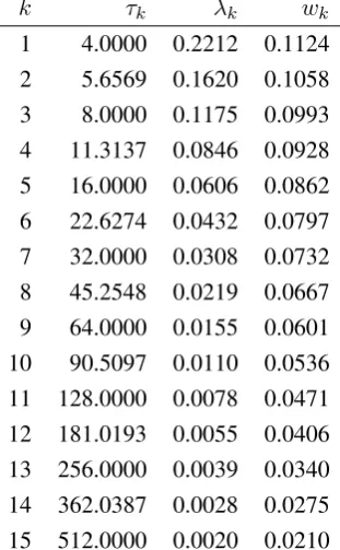
Finally, in the current empirical implementation the valueK is chosen so that τK = 512, which
givesK = 15. Table 1 reports the values of the time horizons, the smoothing constants of theK
[image:8.595.227.383.284.536.2]EWMAs, and the combination weights for the current implementation of RM2006.
Table 1: RM2006: values of the time horizons τk, the corresponding smoothing constants,λk =
1−exp(−τk−1)and the weightwk, proportional to1−lnlnττk0.
k τk λk wk
1 4.0000 0.2212 0.1124 2 5.6569 0.1620 0.1058
3 8.0000 0.1175 0.0993 4 11.3137 0.0846 0.0928 5 16.0000 0.0606 0.0862
6 22.6274 0.0432 0.0797 7 32.0000 0.0308 0.0732
8 45.2548 0.0219 0.0667 9 64.0000 0.0155 0.0601 10 90.5097 0.0110 0.0536
11 128.0000 0.0078 0.0471 12 181.0193 0.0055 0.0406
13 256.0000 0.0039 0.0340 14 362.0387 0.0028 0.0275 15 512.0000 0.0020 0.0210
Denoting w†j = PK
k=1wkλk(1− λk), so that y˜t+1|t = Pjw †
jyt−j, the weights attached to
past observations are an arithmetic weighted average of those arising from EWMAs with different smoothing constants and are no longer a geometric sequence. For l ≥ 1, multistep volatility prediction is carried out by multiplyingy˜t+1|tby the square root of the forecast horizon.
Recalling that the RM1994 volatility prediction is based on a single EWMA with parameter
4
Exponential smoothing for long memory processes
In this section, after discussing several possible interesting extensions of ES that can be envisaged in the long memory case, some of which are based on the structural decomposition into an underly-ing level and a noise component, whereas others are based on the reduced form integrated movunderly-ing average representation, we turn our attention to the FerIMA model.
4.1
Fractional Local Level Model
As it is well known (see, e.g. Harvey, 1989), ES provides the minimum mean square estimator (MMSE) of the level component of the unobserved components model yt = µt+ǫt, where the
level component, µt, evolves as a random walk, µt = µt−1 +ηt, ηt ∼ IID N(0, σ2η), and ǫt ∼
IID N(0, σ2
ǫ), with E(ηsǫt) = 0,forallt, s.
Hence, we may think of replacing µt by a fractional noise process, giving the following
frac-tional local level model (fLLM)
yt=µt+ǫt, (1−B)dµt=ηt,
ǫt ηt ! ∼N " 0 0 ! , σ 2 ǫ 0
0 σ2
η
!#
, t= 1, . . . , n.
Estimation of d and of the noise-signal variance ratio σ2
ǫ/ση2 by frequency domain and wavelet
methods has been considered in Tanaka (2004). Deo and Hurvich (2001) have investigated the estimation of d via log-periodogram regression, whereas Arteche (2004) has focused on local Whittle estimation.
The main difficulty with the fLLM is signal extraction. Applying the Wiener-Kolmogorov filter (see Whittle, 1983, chapter 5 and section 8.5), the MMSE of the underlying fractional noise, assuming the availability of a doubly infinite sample, is
˜
µt|∞ =
1 1 + σǫ2
σ2
η(1−B)
d(1−B−1)dyt.
The above filter encompasses two-sided exponential smoothing (d = 1) and the Hodrick and Prescott (1991) filter (d = 2). The MMSE of the level based on a semi-infinite sample (also said the concurrent or real time estimator) is (Whittle, 1983, p. 58).
mt =
ϕ(1)
ϕ(B)
ϕ(1)
ϕ(B−1)
+
yt,
where ϕ(B)ϕ(B−1)σ2 = σ2
η +σǫ2(1−B)d(1−B−1)d and the operator [h(B)]+ defines a lag
polynomial containing only nonnegative powers of B, i.e. if h(B) = Pb
then[h(B)]+ = Pbj=0hjBj. For fractionald, the above expressions are complicated and do not
provide the signal extraction weights in closed form. The easiest way to address signal extraction and forecasting with the fLLM is to approximate the processµtby a finite order Markovian process
as in Chan and Palma (1998).
4.2
ARFIMA(0,
d
, 1) process
The ARFIMA(0,d,1) process(1−B)dy
t= (1−θB)ξt, ξt ∼IID N(0, σ2),where we assume that
0 ≤ θ < 1, admits the orthogonal decomposition into two orthogonal fractional noise processes integrated respectively of orderdandd−1:
yt=
ηt
(1−B)d +
ǫt
(1−B)d−1,
ǫt ηt ! ∼N " 0 0 !
, σ2 (1−θ)
2 0
0 θ
!#
, t= 1, . . . , n.
This results from writing(1−θB)ξt=ηt+ (1−B)ǫt.
Ifµtdenotes the first component, then the MMSE based on a doubly infinite sample is
˜
µt|∞ =
(1−θ) (1−θB)
(1−θ) (1−θB−1)yt.
This is a two-sided EWMA which depends only on the MA parameter. The second FN(d −1) process is extracted by the filter (1θ(1−θB−B)(1)(1−θB−B−−11)).
The real time signal extraction filter is again ES: as a matter of fact, writing (1− θB) = (1− θ) + θ∆, yt = mt +et, where (1−B)dmt = (1 − θ)ξt can be written in terms of the
observations, mt = [(1−θ)/(1−θB)]yt, i.e. an EWMA of the current and past observations.
Moreover,et = θξt/(1−B)d, and in terms of the observed time series, et = 1−θBθ (1−B)yt, is
proportional to the same EWMA filter applied to the first differences.
Hence, the peculiar trait of this model is that signal extraction takes place by ES, regardless of thedparameter. In the cased = 1we obviously obtain ES, whereas ford = 2we decompose an IMA(2,1) process into an integrated RW and a RW. The forecasts are however dependent on the long memory parameter and would not take the form of exponential smoothing. In particular, the one-step-ahead predictor is given by the recursive formula
˜
yt+1|t= − ∞
X
j=0
Γ(j−d)
Γ(−d)Γ(j+ 1) −θ !
yt−j +θy˜t|t−1.
Notice also thatetis predictable from its past (it is an FN(d−1) process). Also, ifd ∈ (0,1)the
4.3
Fractional Lag IMA(1,1)
Consider the following fractional lag IMA(1,1) model:
(1−B)dyt = (1−θBd)ξt, 0≤θ < 1,
where the fractional lag operator,Bd, is defined asBd= 1−(1−B)d. This is a generalization of
the lag operator to the long memory case originally proposed by Granger (1986) and it has been recently adopted by Johansen (2008) to define a new class of vector autoregressive models.
The above specification provides an interesting extension of ES to the fractional case. In fact, the process admits the decomposition into a fractional noise component and a WN component:
yt=mt+et, mt=
1−θ
(1−B)dξt, et =θξt.
In terms of the observations,
mt=
1−θ
1−θBd
yt
which is the ES in the cased= 1. In the cased = 2, the model is the basis for the decomposition ofytinto an integrated random walk plus a noise component (the reduced form being(1−B)2 =
(1−2θB+θ2B2)ξ
t).
4.4
Fractional Equal Root Moving Average Process
In his seminal Biometrika paper, Hosking (1981) introduced the fractional equal–root integrated moving average process
(1−B)dyt= (1−θB)dξt, ξt∼WN(0, σ2). (6)
Writing1−θB= (1−θ)−θ(1−B)and using the binomial expansion of[(1−θ)−θ(1−B)]d,
the process (6) admits the following decomposition:
yt = P∞j=0zjt, zjt = (dj)!j 1−θθ
j 1−θ
1−θB
d
(1−B)jy
t (7)
where (d)j = d(d− 1)· · ·(d− j + 1) is the Pochhammer symbol. This is an infinite sum of
generalized EWMAs applied toytand its successive differences.
The first component is the weighted moving average of the observations available at timet:
z0t =
1−θ
1−θB
d
yt= ∞
X
j=0
with weights given by
w∗j = (1−θ)dϕj, ϕj =−θ
1
j(1−d−j)ϕj−1, j >0, ϕ0 = 1,
by application of Gould’s formula (Gould, 1974), or
wj∗ = (1−θ)dθ
j
j!d
(j), (9)
whered(j)denotes the rising factoriald(j) =d(d+ 1)· · ·(d+j −1).
In terms ofλ = 1−θ,
w∗j =wjcj, wj =λ(1−λ)j, cj =
λd−1d(j)
j! , (10)
which shows that the weights result from correcting the geometrically declining weights, wj =
(1−λ)wj−1, w0 = 1, by a factor depending ond, decreasing hyperbolically withj:
cj =
1− 1−d
j
, c0 =λd−1.
The importance of the correction term is larger, the smaller isλ, due to the factorλd−1. Moreover,
ifd= 1, λd−1d(j)
j! = 1.
We label the linear filter[(1 −θ)/(1−θB)]din (8) a fractional exponential smoothing (FES)
filter. Section 6 will provide a discussion of its properties. The filter performs a long memory -EWMA of the available observations. It depends on two parameters, the memory parameter, d, and the parameterθ, which regulates the speed of mean reversion.
According to (12) the processytis decomposed as the sum of fractionally integrated processes
of orderd−j, j = 0,1, . . . .
zjt = (dj)!jθj(1−θ)j−d(1−B)jP∞k=0 Γ(Γ(k+1)Γ(k+d)d)ξt−k (11)
The components, fordin certain ranges, can be interpreted as the underlying level (z0t), the
under-lying slope (z1t), acceleration (z2t), etc., as it will be discussed in the next section. For a stationary
long memory process,z0tis the fractional noise process,(1−B)dz0t= (1−θ)dξt, whereasz1tis
the antipersistent process(1−B)d−1z
1t=dθ(1−θ)d−1ξt, etc. To extract thej-th component, the
filter(1−θB)−d = P
jϕjBj, ϕj = θ
j
j!d
(j), is applied to the series(1−B)jy
t, and the outcome
is rescaled by(d)jθj(1−θ)d−j. The filters can be approximated by truncating the weights at lag
Ifdis integer, then the number of components is finite. Whend= 1,
yt=z0t+z1t, (1−B)z0t= (1−θ)ξt, z1t =θξt,
and the two components can be interpreted as the permanent and the transitory components in the series (see the next section).
Whend = 2,
yt=z0t+z1t+z2t, (1−B)2(z0t+z1t) = (1−θB)(1−θ)ξt, z3t =θ2ξt
so thatz0t is a stochastic level (an integrated RW), which is coincident with double exponential
smoothing (Brown, 1963). The latter is the optimal predictor for the IMA(2,2) process with a MA rootθ−1 with multiplicity 2;z
1t is a stochastic slope (a RW), and their sum is IMA(2,1), and the
processz2tis white noise.
The next section discusses the interpretation of the components and their relation with the mul-tistep predictor.
5
Permanent-Transitory (Beveridge and Nelson)
Decomposi-tion
The decomposition of the FerIMA process proposed above arises as a special case of the following result, which can be viewed as a generalization of the Beveridge and Nelson (1981, BN hence-forth).
Assumed >0and letytbe the (possibly fractionally) integrated process
∆dyt=ψ(B)ξt, ψ(B) = 1 +ψ1B+ψ2B2+· · ·,
X
j
ψj2 <∞,
andξt∼WN(0, σ2). Consider the expansion of the Wold polynomial
ψ(B) =
r−1
X
j=0
ψj(1)(1−B)j +ψr(B)(1−B)r,
where
ψj−1(B) =ψj−1(1) + ∆ψj(B), j = 1,2, . . . , ψ0(B) =ψ(B).
Two interesting particular cases arise:
• Ifψ(B) = 1 +ψ1B +· · ·+ψqBq, an MA(q) polynomial, then, if r = q, ψr(B)is a zero
• Ifψ(B)is an ARMA(p, q) polynomial, thenψr(B)is an ARMA(p,min{(p−r),(q−r)})
polynomial. Consider for simplicity the case whenq ≥ p, so that, defining θ(B) = 1 −
θ1B− · · · −θqBq andφ(B) = 1−φ1B− · · · −φpBp, we can write
ψ(B) = θ(B)
φ(B) =
θ0(1) +θ1(1)(1−B) +· · ·+θq(1)(1−B)q
φ(B)
we have that forr≤q,
ψr(B) =θr(1) +θr+1(1−B) +· · ·+θq(1)(1−B)q−r,
i.e. an MA(q−r) lag polynomial.
For a given integerr >0, the following decomposition is valid:
yt=z0t+z1t+· · ·zr−1,t+ ˜zrt, (12)
where
zjt =
ψj(1)
(1−B)d−jξt, j = 0, . . . , r−1,
is an FN(d−j) process, and
˜
zrt=
ψr(B)
(1−B)d−rξt.
For integer d = r > 0, z˜r,t is a stationary short memory process, with ARMA(p,min{(p−
r),(q− r)} representation if ψ(B) is ARMA(p, q), and can be referred to as the BN transitory component, as its prediction converges fastly to zero as the forecast horizion increases. The sum Pd−1
j=0zjt is the long run or permanent component, as it represents the value that the series would
take if it were on the long run path, i.e. the value of the long run forecast function actualised at timet.
More generally, for both fractional and integer values of d, we set r = [d], where [d] is the nearest integer tod, in the expression (12) to obtain a generalized BN decomposition:
yt=mt+et, mt=z0t+· · ·+z[d]−1,t, et =
ψr(B)
(1−B)d−[d]ξt.
The component mt is the nonstationary component, determining the behaviour of the forecast
function for long multistep horizons. The component et is stationary, its integration order being
d−[d]∈(−0.5,0.5).
• Whend ∈ [0,0.5)the componentmtis identically equal to zero and all the series is
transi-tory. In fact,[d] = 0and the multistep forecast takes the form
˜
yt+l|t=
ψ(B) (1−B)dB
−l
+
ξt. (13)
• Whend∈(0.5,1.5),ytadmits the following nonstationary-stationary decomposition:
yt =mt+et, mt=z0t, et=
ψ1(B)
(1−B)d−1ξt
Ifd = 1andψ(B) = (1−θB), then mt is an EWMA ofyt andet is white noise. Notice
that ford ∈[0.5,1)the long run forecast of the series is zero and the shocks(1−θ)ξthave
long lasting, but transitory effects. Hence mt is not equivalent its long run prediction, i.e.
the value the series would take if it were on its long run path.
• Whend∈(1.5,2.5),ytadmits the following nonstationary-stationary decomposition:
yt =mt+et, mt =z0t+z1t, et=
ψ2(B)
(1−B)d−2ξt
Ifd = 2andψ(B) = (1−θ1B −θ2B2), thenmtcan be computed according to the
Holt-Winters recursive formulae (see Harvey, 1989) andetis white noise.
• In general, the component et is a stationary process featuring long memory (d > [d]) or
antipersistence (d <[d]).
It should be noticed that the above decomposition differs from the one proposed by Ari˜no and Marmol (2004) for nonstationary fractional processes withd∈ (0.5,1.5). The latter is based on a different interpolation argument and decomposesyt = m∗t +e∗t, where, in terms of our notation,
e∗ t =
ψ1(B)
Γ(d) ξt.As a result, their permanent component is
m∗
t =yt−e∗t =z0t+
1 Γ(d)
Γ(d)(1−B)1−d−1
ψ1(B)ξt.
Thus, it contains a purely short memory component and in the case d ∈ (0.5,1)differs from the long run prediction of the series, which is equal to zero.
6
Fractional Exponential Smoothing Filters
Letting w(B) = P
wjBj denote a generic linear filter, we denote its transfer function by
G(ω) = w(e−ıω), e−iω = cosω −ısinω, where ı is the imaginary unit and ω ∈ [0, π] is the
angular frequency in radians. As it is well known, see for instance Percival and Walden (1993), the gain function, |G(ω)|, provides a useful characterisation about how the linear filter modifies the amplitude of the cyclical components in the series. A low-pass filter is a filter that passes low frequency fluctuations and reduces the amplitude of fluctuations with frequencies higher than a cutoff frequency ωc (see e.g. Percival and Walden, 1993). The latter is defined as the angular
frequency at which a monotonically decreasing gain is equal to 1/2. Correspondingly, the filter is said to pass the fluctuations with period greater than2π/ωc and suppress to a large extent (e.g.
compress by a factor small than 0.5) those with smaller period (ω > ωc). The cutoff frequency or
period is a useful summary measure for defining the characteristic properties of a low-pass filter, although it is not the unique, as we shall see immediately.
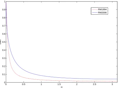
Figure 3 compares the gains of the two Riskmetrics filters, RM1994 and RM2006. The cutoff frequency is very close, being equal toωc = 0.0889for RM1994 andωc = 0.0765, which
corre-spond to a period of 70.69 and 82.13 observations, respectively. However, the RM1994 filter is more concentrated at the cutoff. The concentration can be measured by
β2(ωc) =
Rωc
0 |G(ω)| 2dω
Rπ
0 |G(ω)|2dω
The above concentration measure was defined and analysed according to different perspectives by Tufts and Francis (1970), Papoulis and Bertran (1970), Eberhard (1973) and Slepian (1978). As a result, the RM2006 volatility estimate will be slightly smoother than RM1994. However, the output of the filters will be very similar.
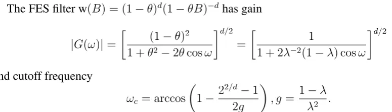
The FES filter w(B) = (1−θ)d(1−θB)−dhas gain
|G(ω)|=
(1−θ)2
1 +θ2−2θcosω
d/2 =
1
1 + 2λ−2(1−λ) cosω
d/2
and cutoff frequency
ωc = arccos
1− 2
2/d−1
2g
, g = 1−λ
[image:16.595.78.466.498.609.2]λ2 .
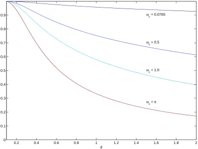
Figure 2 displays the combinations ofdandθ, respectively in the interval (0,2] and [0,1], giving the same cutoff frequencyωc, for some values ofωc. The curve forωc = 0.0765provides the
com-binations that will deliver filtered estimates with comparable smoothness with respect to RM2006; for instance, we needd = 0.7,θ = 0.98to obtain a similar filter. Other cutoff frequencies taken into consideration areωc = 0.5, corresponding to a period of 13 observations,ωc = 1,
Figure 1: Plot of the gains of the RM1994 and RM2006 filters versus the angular frequencyω.
0 0.5 1 1.5 2 2.5 3
0 0.1 0.2 0.3 0.4 0.5 0.6 0.7 0.8 0.9 1
ω
G
a
in
RM1994 RM2006
stationary values of d and θ less than 0.5 the FES filter is an all-pass filter (i.e. |G(π)| < 0.5), and in order to obtain a substantial amount of smoothing we need to haveθvery close to 1. Small variations of theθparameter in the neighbourhood of 1 cause big changes of the cutoff frequency. Obviously,d= 1,θ= 0.94yields the RM1994 ES filter.
7
Estimation and Forecasting with the FerIMA model
lettingωj = 2πjn , j= 1, . . . ,⌊n−21⌋,denote the Fourier frequencies, where⌊·⌋is the largest integer
not greater than the argument, the periodogram, or sample spectrum, is defined as
I(ωj) =
1 2πn n X t=1
(yt−y¯)e−ıωjt
2 ,
wherey¯=n−1Pn
t=1yt.
Letting
f(ω) = 1 2π
1 +θ2−2θcosω
2(1−cosω) p
σ2
denote the (pseudo) spectral density ofyt, the Whittle likelihood is:
ℓ(d, θ, σ2) =−
⌊(n−1)/2⌋
X
j=1
lnf(ωj) +
I(ωj)
f(ωj)
. (14)
The maximiser of (14) is the Whittle pseudo maximum likelihood estimator of (d, θ, σ2). We
refer to Dahlhaus (1989), Giraitis, Koul and Surgailis (2012), and Beran et al. (2013) and for the properties of the estimator in the long memory case. In the nonstationary case, the consistency and the asymptotic normality of the Whittle estimator has been proven by Velasco and Robinson (2000). Tapering may be needed to eliminate polynomial trends, see Velasco and Robinson (2000), but we do not contemplate this possibility here. Notice that we have excluded the frequencies
ω= 0, andπfrom the analysis; the latter may be included with little effort, and their effect on the inferences is negligible in large samples.
The l-step-ahead forecast of the FerIMA model is obtained from each components forecasts, i.e. y˜t+l|t = Pjz˜j,t+l|t.The components are characterised by decreasing levels of predictability:
in fact, the prediction error variance increases with the order of the component,j.
Alternatively, the predictor can be obtained directly from the model specification. Denoting byy¯t = t−1Pt−j=01yt−j, the mean of the available sample observations at time t, thel-steps-ahead
predictor ofytis
˜
yt+l|t = ¯yt+Pjt−=01πjl(yt−j −y¯t),
= Pt−1
j=0πjl∗yt−j, πjl∗ =πjl+1t(1−πjl).
The weightsπjl are computed by the Durbin-Levinson algorithm (see e.g. Palma, 2007) and in
large sample they are obtained as follows:
πjl= l−1
X
i=0
ψiπj+l−i
whereψiis the coefficient of the Wold polynomial associated toBi, yt =ψ(B)ξtandπ(B)is the
8
The Empirical Performance of the FerIMA Volatility
Predic-tor
We consider the empirical problem of forecasting one-step-ahead the daily asset returns volatility, using realized measures constructed from high frequency data. The volatility proxy is the Realized Variance (5-minute) of 21 stock indices extracted from the database ”OMI’s realized measure library” version 0.2, produced by Heber, Lunde, Shephard, and Sheppard (2009). The background information for realized measures can be found in the survey articles by by McAleer and Medeiros (2008) and Andersen, Bollerslev and Diebold (2010). The series range from 03/01/2000 to the 22/01/2014 for a total of 3,674 daily observations.
Denoting byRVta generic realized volatility series, we focus on its logarithmic transformation,
that is we takeyt = lnRVt. We are interested in assessing the properties of the FerIMA predictor
discussed in the previous section, in comparison to three well established alternative: RM1994, which is the standard exponential smoothing predictor withλ= 0.06, the RM2006 methodology, and the heterogeneous autoregressive (HAR) model proposed by Corsi (2009), which is specified as follows:
yt=φ0+φ1yt−1+φ5y¯t−5+φ22y¯t−22+ξt, ξt∼WN(0, σ2),
where
¯
yt−5 =
1 5
5
X
j=1
yt−j,y¯t−22=
1 22
22
X
j=1
yt−j,
are respectively the average realized variance over the previous trading week and over the previous month. This specification captures the long memory feature of RV via a long autoregression, yet preserving the parsimony, and has proven to be very effective for forecasting volatility, rapidly becoming one of the discipline’s standards.
We perform a recursive forecasting experiment such that starting from timen0 = 500we
com-pute the one step ahead volatility predictions according to the four methods and we proceed adding one observation at time. For the HAR And FerIMA specifications we re-estimate the parameters each time a new observation is added. The experiment yields 3,174 one step ahead prediction errors for each forecasting methodology to be used for the comparative assessment.
Denoting by y˜k,t|t−1 the prediction arising from method k, where k is an element of the set {RM1994, RM2006, HAR, F}, F standing for FerIMA, and byvk,t=yt−y˜k,t|t−1,the
correspond-ing prediction error,t=n0+ 1, . . . , n,we compare the mean square forecast error,
MSFEk=
1
n−n0
n
X
t=n0+1
and compute the Diebold-Mariano-West test of equal forecasting accuracy. Denotingdk,t=vk,t2 −
v2
F,t the quadratic loss differential, the Diebold-Mariano-West test of the null hypothesis of equal
forecast accuracy,H0 : E(dk,t) = 0, versus the one sided alternativeH1 : E(dkt) > 0, is the test
statistic
DMk =
¯
dk
p
σ2
k
, d¯k =
1
n−n0
n
X
t=n0+1
dk,t, σk2 =
1
n−n0
"
c0+ 2
J−1
X
j=1
J −j J cj
#
,
wherecj is the sample autocovariance of dk,t at lag j andσk2 is a consistent estimate of the long
run variance of the loss differential. We set the truncation lag equal toJ = 22. See Diebold and Mariano (1995) and West (1996). The null distribution of the test is Student’st withn−n0−1
degrees of freedom.
The results for the 21 realized volatility series (yt = lnRVt) are reported in table 2. The
FerIMA predictor is characterised by a lower MSFE and systematically outperforms the RM1994 and RM2006 predictors, with a single exception (All Ord. series). Only in 3 out of 21 cases the HAR predictor has a lower MSFE. In terms of the Diebold-Mariano-West test, we reject the null that the RM1994 and RM2006 predictors have the same forecast accuracy as the FerIMA predictor at the 5% significance level in all but two cases (All Ord.andHang Seng). When the HAR predictor is compared to the FerIMA predictor, we do not reject in four cases (All Ord.,DIJA,Hang Seng, and IPC Mexico).
Hence, the evidence is strongly in favour of the FerIMA predictor. We also observe that the performance of RM2006 does not differ substantially from RM1994, since, as it was anticipated in section 6, the two predictors are very similar. Also, HAR systematically outperforms both RiskMetrics predictors.
The last two columns of the table report the values of the estimated FerIMA parametersθandd. The memory parameter is always in the nonstationary region (the average of the estimated values being 0.60, with standard deviation 0.04), whereas the moving average parameter ranges from 0.21 to 0.65 with an average value 0.36 and standard deviation 0.12.
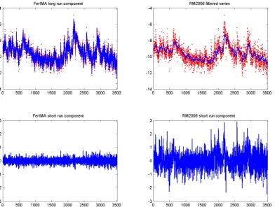
Figure 3 displays the logarithm of the realized volatility series for the S&P 500 index, along with the RM2006 filtered series and the componentmt = z0textracted from the FerIMA model,
computed according to 8, replacing the unknown parameters by their maximum likelihood esti-mates d˜= 0.56 and θ˜ = 0.35. The bottom left plot is the stationary componentyt−mt = et
and the bottom right plot is the deviation from the RM2006 filtered series. It is noticeable that a substantial part of the variation ofytis absorbed by the componentz0t, whereas RM2006 seems to
Table 2: Log-Realized volatility series. Recursive forecasting exercise: comparison of one-step-ahead predictive performance. The first three columns present the relative MSFE ratios MSFEF
MSFERM2006,
MSFEF
MSERM1994,
MSFEF
MSFEHAR, respectively. The next three
columns report the p-values of the Diebold-Mariano test of equal forecast accuracy versus the alternative that the FerIMA (abbreviated to F) is more accurate.
Relative Mean Square Forecast Error p-values of DM test
Series F vs RM2006 F vs RM1994 F vs HAR F vs RM2006 F vs RM1994 F vs HAR d˜ θ˜
S&P 500 0.84 0.85 0.96 0.000 0.000 0.070 0.63 0.44
FTSE 100 0.74 0.76 0.88 0.000 0.000 0.000 0.65 0.35
Nikkei 225 0.76 0.75 0.84 0.000 0.000 0.000 0.55 0.23
DAX 0.75 0.77 0.87 0.000 0.000 0.000 0.61 0.29
Russel 0.86 0.86 0.95 0.000 0.000 0.021 0.58 0.41
All Ord. 1.03 1.04 1.09 0.833 0.887 1.000 0.64 0.65
DJIA 0.91 0.91 1.01 0.016 0.017 0.694 0.65 0.50
Nasdaq 100 0.75 0.75 0.83 0.000 0.000 0.000 0.59 0.21
CAC 40 0.75 0.76 0.88 0.000 0.000 0.000 0.62 0.31
Hang Seng 0.97 0.98 1.04 0.255 0.341 0.935 0.64 0.55
KOSPI Composite Index 0.76 0.76 0.86 0.000 0.000 0.000 0.61 0.27
AEX Index 0.73 0.74 0.87 0.000 0.000 0.000 0.63 0.31
Swiss Market Index 0.73 0.76 0.91 0.000 0.000 0.001 0.66 0.36
IBEX 35 0.75 0.75 0.85 0.000 0.000 0.000 0.58 0.26
S&P CNX Nifty 0.81 0.79 0.85 0.000 0.000 0.000 0.53 0.26
IPC Mexico 0.94 0.94 0.98 0.030 0.020 0.141 0.55 0.50
Bovespa Index 0.80 0.79 0.87 0.000 0.000 0.000 0.51 0.23
S&P/TSX Composite Index 0.87 0.88 0.92 0.003 0.002 0.002 0.57 0.40
Euro STOXX 50 0.82 0.82 0.91 0.000 0.000 0.001 0.60 0.37
FT Straits Times Index 0.82 0.83 0.88 0.000 0.000 0.000 0.58 0.36
9
Conclusions
We have dealt with the problem of forecasting volatility and decomposing it into meaningful com-ponents in the presence of long memory and possible nonstationarity.
We have reviewed the solutions available in the literature and have concluded that the recent RM2006 yields results that are not substantially different from the exponential smoothing predictor with fixed smoothing constant known as RM1994. From the point of view of signal extraction, when applied to realized volatility series (rather than squared or absolute returns or similar noisy proxies), both methodologies yield estimates of underlying volatility that are very stable and imply a very smooth estimate.
After reviewing some plausible extensions of ES to the fractionally integrated framework, we have looked at the properties of a signal extraction filter and the predictor arising from the FerIMA model, a specification originally formulated by Hosking (1981), proposing a decomposition into fractional noise components of decreasing order and offering an interpretation in the light of the well known Beveridge and Nelson decomposition.
A forecasting experiment has illustrated the potential of the FerIMA model for forecasting daily realized volatility, showing that it outperforms both RiskMetrics predictors and the Heterogeneous Autoregressive Model.
In conclusion, the FerIMA model is a simple and parsimonious model, which can play a useful role in forecasting volatility and extracting its underlying level.
Acknowledgements
The author thanks Federico Carlini at CREATES for discussion on the fractional lag operator. The author gratefully acknowledge financial support by the Italian Ministry of Education, Univer-sity and Research (MIUR), PRIN Research Project 2010-2011 - prot. 2010J3LZEN, ”Forecasting economic and financial time series” and from CREATES - Center for Research in Econometric Analysis of Time Series (DNRF78), funded by the Danish National Research Foundation.
References
[2] Amado, C., and Ter¨asvirta, T. (2013). Modelling volatility by variance decomposition.Journal of Econometrics, 175, 142-153.
[3] Amado, C., and Ter¨asvirta, T. (2014). Modelling changes in the unconditional variance of long stock return series.Journal of Empirical Finance, 25(C), 15-35.
[4] Andersen, T.G., Bollerslev, T., and Diebold, F.X. (2010). Parametric and Nonparametric Volatility Measurement. In Y. A¨ıt-Sahalia and L.P. Hansen (eds.), Handbook of Financial Econometrics, Chapter 2, pp. 67-128. Amsterdam: Elsevier Science B.V.
[5] Andersen, T.G., Bollerslev, T., Diebold, F.X., Labys, P. (2003). Modeling and forecasting realized volatility.Econometrica, 71, 579-625.
[6] Andersen, T.G., Bollerslev, T., Diebold, F.X., Labys, P. (2001). The Distribution of Exchange Rate Volatility.Journal of the American Statistical Association, 96, 4255.
[7] Arteche, J. (2004). Gaussian Semiparametric Estimation in Long Memory in Stochastic Volatility Models and Signal plus Noise Models.Journal of Econometrics, 119, 131-154.
[8] Beran, J., Feng, Y., Ghosh, S. and Kulik, R. (2013), Long-Memory Processes Probabilistic Properties and Statistical Methods, Springer-Verlag Berlin Heidelberg.
[9] Bauwens, L., Hafner, C.M., and Pierret, D. (2013). Multivariate Volatility Modeling of Elec-tricity Futures.Journal of Applied Econometrics, 28, 743 761.
[10] Beveridge, S., and Nelson, C.R. (1981). A new approach to decomposition of economic time series into permanent and transitory components with particular attention to measurement of the business cycle.Journal of Monetary Economics, 7, 151 174.
[11] Bollerslev, T. and Wright, J.H. (2000). Semiparametric Estimation of Long-Memory Volatil-ity Dependencies: The Role of High Frequency Data.Journal of Econometrics, 98, 81106.
[12] Brown, R.G. (1963). Smoothing, Forecasting and Prediction of Discrete Time Series. NJ: Prentice-Hall, Englewood Cliffs.
[13] Chan, N. H. and Palma, W. (1998). State Space Modeling of Long-Memory Processes. The Annals of Statistics, 26, 719–740.
[15] Corsi, F. (2009). A simple long memory model of realized volatility. Journal of Financial Econometrics, 7, 174-196.
[16] Cox, D. R. (1961). Prediction by exponentially weighted moving averages and related meth-ods.Journal of the Royal Statistical Society, Series B, 23, 414-422.
[17] Dahlhaus, R. (1989). Efficient Parameter Estimation for Self Similar Processes.The Annals of Statistics, 17, 4, 1749-1766.
[18] Deo, R.S. and Hurvich, C.M. (2001). On the log periodogram regression estimator of the memory parameter in long memory stochastic volatility models.Econometric Theory, 17, 686-710.
[19] Diebold, F. X. and Inoue, A. (2001). Long memory and regime switching.Journal of Econo-metrics, 105, 131–159.
[20] Diebold, F. X. and Mariano, R. (1995). Comparing predictive accuracy.Journal of Business & Economic Statistics, 13, 253 - 263.
Ding, Z., and Granger, C. W. J. (1996). Modeling Volatility Persistence of Speculative Returns: A New Approach, Journal of Econometrics, 73, 185 215.
[21] Ding, Z., Granger, C. W. J., and Engle, R.F. (1993). A Long Memory Property of StockMarket Returns and a New Model.Journal of Empirical Finance, 1, 83106.
[22] Engle, R.F. (1995).ARCH: Selected Readings. Oxford University Press, 1995.
[23] Engle, R.F., Ghysels, E., and Sohn, B. (2013). Stock market volatility and macroeconomic funda- mentals.Review of Economic and Statistics, 95, 776797.
[24] Engle, R.F., and Lee (1999). A Long-Run and Short-Run Component Model of Stock Re-turn Volatility. In Engle, R.F., and White, A. (eds),Cointegration, Causality, and Forecasting, Oxford University Press. Oxford, UK.
[25] Gallant, A.R., Hsu, C.T. and Tauchen, G. (1999). Using Daily Range Data to Calibrate Volatility Diffusions and Extract the Forward Integrated Variance, Review of Economics and Statistics, 81, 617 - 631.
[27] Gardner, E.S. (2006). Exponential smoothing: the state of the art. Part II.International Jour-nal of Forecasting, 22, 637-666.
[28] Giraitis, L., Koul, H.L., Surgailis, D. (2013),Large Sample Inference for Long Memory Pro-cesses, Imperial College Press.
[29] Gould, H. W. (1974). Coefficient Identities for Powers of Taylor and Dirichlet Series. Amer-ican Mathematical Monthly, 81, 3 14.
[30] Giraitis, L., Koul, H. and Surgailis, D. (2012). Large Sample Inference for. Long memory Processes, Imperial College Press, London.
[31] Granger, C.W.J. (1980). Long memory relationships and the aggregation of dynamic models. Journal of Econometrics, 14, 227238.
[32] Granger, C.W.J. (1986). Developments in the study of cointegrated economic variables. Ox-ford Bulletin of Economics and Statistics, 48, 213-228.
[33] Granger, C.W.J., and Hyung, N. (2004). Occasional Structural Breaks and Long Memory with an Application to the S&P 500 absolute returns. Journal of Empirical Finance, 11, 399 – 421.
[34] Granger, C.W.J., and Joyeux, R. (1980). An introduction to long memory time series models and fractional differencing, Journal of Time Series Analysis, 1, 15 - 29.
[35] Gray, H.L., Woodward, W. A. and Zhang, N. (1989). On Generalized Fractional Processes. Journal of Time Series Analysis, 10, 233–257.
[36] Hafner, C., and Linton, O.B. (2010). Efficient estimation of a multivariate multiplicative volatility model.Journal of Econometrics, 159, 5573.
[37] Harvey, A. C. (1989). Forecasting, Structural Time Series Models and the Kalman Filter. Cambridge: Cambridge University Press.
[38] Heber, G., Lunde, A., Shephard, N. and Sheppard, K. K. (2009). OMIs realised measure library. Version 0.2, Oxford-Man Institute, University of Oxford.
[40] Hodrick, J. R., Prescott E. C. (1997). Postwar U.S. business cycles: an empirical investiga-tion.Journal of Money, Credit and Banking, 29, 116.
[41] Hosking, J.R.M. (2006). Fractional differencing.Biometrika, 88, 168-176.
[42] Hurvich, C.M., and Ray, B.K. (2003). The Local Whittle Estimator of Long-Memory Stochastic Volatility.Journal of Financial Econometrics, 1, 445–470.
[43] Johansen, S. (2008). A representation theory for a class of vector autoregressive models for fractional processes.Econometric Theory, 24, 651 676.
[44] McAleer, M. and Medeiros, M. C. (2008). Realized Volatility: A Review. Econometric Re-views, 27, 10–45.
[45] Palma, W. (2007).Long-memory Time Series: Theory and Methods. Wiley. Hoboken, New Jersey.
[46] Percival D., Walden A. (1993).Spectral Analysis for Physical Applications. Cambridge Uni-versity Press.
[47] Pillai, T.R., Shitan. M. and Peiris, M.S. (2012) Some Properties of the Generalized Autore-gressive Moving Average (GARMA (1,1;δ1,δ2)) Model. Communications in Statistics - Theory
and Methods, 41, 699–716.
[48] Proietti, T., and Luati A. (2012). Generalised Linear Spectral Models. Forthcoming in Shep-hard, N. and Koopman, S.J. (2014), Unobserved Components and Time Series Econometrics, Oxford University Press, Oxford, UK.
[49] RiskMetrics Group (1996). RiskMetrics Technical Document, New York: J.P. Mor-gan/Reuters
[50] Shephard, N. (2005).Stochastic Volatility: Selected Readings. Oxford University Press.
[51] Slepian D., Pollak H.O. (1961), Prolate Spheroidal Wave Functions, Fourier Analysis and Uncertainty, I,The Bell System Technical Journal, 40, 43-64.
[53] Tanaka, K. (2004). Frequency domain and wavelet-based estimation for long-memory signal plus noise models. In A. Harvey. S.J. Koopman and N. Shephard (eds.),State Space and Un-observed Component Model. Theory and Application, ch. 4, p. 75–91, Cambridge University Press. 13, 109–131.
[54] Tiao, G. C., and Tsay, R. S. (1994). Some advances in non-linear and adaptive modeling in time-series. Journal of Forecasting, 13, 109–131.
[55] Tiao, G.C., and Xu, D. (1993). Robustness of maximum likelihood estimates for multi-step predictions: the exponential smoothing case.Biometrika, 80, 623 641.
[56] Velasco, C., and Robinson, P.M. (2000), Whittle pseudo-maximum likelihood estimation for non-stationary time series,Journal of the American Statistical Association, 95, 1229-1243.
[57] West, K. (1996). Asymptotic inference about predictive ability, Econometrica, 64, 1067 -1084.
[58] Whittle, P. (1953). Estimation and Information in Stationary Time Series, Arkiv f¨or Matem-atik, 2, 423–434.
[59] Whittle, P. (1983).Prediction and Regulation by Linear Least-square Methods(2nd edition). Basil Blackwell, Oxford, UK.
Figure 2: Combinations ofd(horizontal axis) andθ(vertical axis) giving the same cutoff frequency for FES filter.
d
θ
ωc = 0.0765
ωc = 0.5
ωc = 1.0
ω
c = π
0.2 0.4 0.6 0.8 1 1.2 1.4 1.6 1.8 2