Cross-Validation, Shrinkage and Variable Selection in
Linear Regression Revisited
Hans C. van Houwelingen1, Willi Sauerbrei2
1Department of Medical Statistics and Bioinformatics, Leiden University Medical Center, Leiden, The Netherlands 2Institut fuer Medizinische Biometrie und Medizinische Informatik, Universitaetsklinikum Freiburg, Freiburg, Germany
Email: [email protected]
Received December 8,2012; revised January 10, 2013; accepted January 26,2013
Copyright © 2013 Hans C. van Houwelingen, Willi Sauerbrei. This is an open access article distributed under the Creative Commons Attribution License, which permits unrestricted use, distribution, and reproduction in any medium, provided the original work is properly cited.
ABSTRACT
In deriving a regression model analysts often have to use variable selection, despite of problems introduced by data- dependent model building. Resampling approaches are proposed to handle some of the critical issues. In order to assess and compare several strategies, we will conduct a simulation study with 15 predictors and a complex correlation struc- ture in the linear regression model. Using sample sizes of 100 and 400 and estimates of the residual variance corre- sponding to R2 of 0.50 and 0.71, we consider 4 scenarios with varying amount of information. We also consider two
examples with 24 and 13 predictors, respectively. We will discuss the value of cross-validation, shrinkage and back- ward elimination (BE) with varying significance level. We will assess whether 2-step approaches using global or pa- rameterwise shrinkage (PWSF) can improve selected models and will compare results to models derived with the LASSO procedure. Beside of MSE we will use model sparsity and further criteria for model assessment. The amount of information in the data has an influence on the selected models and the comparison of the procedures. None of the ap- proaches was best in all scenarios. The performance of backward elimination with a suitably chosen significance level was not worse compared to the LASSO and BE models selected were much sparser, an important advantage for inter- pretation and transportability. Compared to global shrinkage, PWSF had better performance. Provided that the amount of information is not too small, we conclude that BE followed by PWSF is a suitable approach when variable selection is a key part of data analysis.
Keywords: Cross-Validation; LASSO; Shrinkage; Simulation Study; Variable Selection
1. Introduction
In deriving a suitable regression model analysts are often faced with many predictors which may have an influence on the outcome. We will consider the low-dimensional situation with about 10 to 30 variables, the much more difficult task of analyzing ‘omics’ data with thousands of measured variables will be ignored. Even for 10+ vari- ables selection of a more relevant subset of these vari- ables may have advantages as it results in simpler models which are easier to interpret and which are often more useful in practice. However, variable selection can intro- duce severe problems such as biases in estimates of re- gression parameters and corresponding standard errors, instability of selected variables or an overoptimistic esti- mate of the predictive value [1-4].
To overcome some of theses difficulties several pro- posals were made during the last decades. To assess the
When building regression models it has to be distin- guished whether the only interest is a model for predic- tion or whether an explanatory model, in which it is also important to assess the effect of each individual covariate on the outcome, is required. Whereas the mean square error of prediction (MSE) is the main criterion for the earlier situation, it is important to consider further quality criteria for a selected model in the latter case. At least interpretability, model complexity and practical useful- ness are relevant [6]. For the low-dimensional situation we consider backward elimination (BE) as the most suit- able variable selection procedure. Advantages compared to other stepwise procedure were given by [7]. For a more general discussion of issue in variable selection and arguments to favor BE to other stepwise procedures and to subset selection procedures using various penalties (e.g. AIC and BIC) see [4] and [8]. To handle the impor- tant issue of model complexity we will use different nominal significance levels of BE. The two post-estima- tion shrinkage approaches mentioned above will be used to correct parameter estimates of models selected by BE. There are many other approaches for model building. Despite of its enormous practical importance hardly any properties are known and the number of informative simulation studies is limited. As a result many issues are hardly understood, guidance to built multivariable regres- sion models is limited and a large variety of approaches is used in practice.
We will focus on a simple regression model
0 1
Y X
,
, ,
n, n
with X a p-dimensional covariate. Let there be n ob- servations y x1 1 Λ y x used to obtain estimates
1
b and 0 x b1
15 p
0
b y of the regression parameters. The standard approach without variable selection is classic ordinary least squares (OLS). In a simulation study we will investigate how much model building can be improved by variable selection and cross-validated based shrinkage. The paper reviews and extends early work by the authors [2,4,9]. Elements added are a tho- rough reflection on the value of cross-validation and a comparison with Tibshirani’s LASSO [5]. With an in- terest in deriving explanatory models we will not only use the MSE as criteria, but will also consider model complexity and the effects of individual variables. Two larger studies analyzed several times in the literature will also be used to illustrate some issues and to compare results of the procedures considered.
The paper is structured in the following way. Section 2 describes the design of the simulation study. Section 3 reviews the role of cross-validation in assessing the pre- diction error of a regression model and studies its be- havior in the simulation study. Section 4 reviews global and parameterwise shrinkage and assesses the perform-
ance of cross-validation based shrinkage in the simu- lation data. The next Sections 5 and 6 discuss the effect of model selection by BE and the usefulness of cross- validation and shrinkage after selection. Section 7 com- pares the performance of post-selection shrinkage with the LASSO. Two real-life examples are given in Section 8. Finally, the findings of the paper are summarized and discussed in Section 9.
2. Simulation Design
The properties of the different procedures are investi- gated by simulation using the same design as in [10]. In
that design the number of covariates , the cova-
riates have a multivariate normal distribution with mean
j , standard deviation j 1
7,14 ,13
0.3, 0.5, 0.5
R R R
0.7
R
for all covariates. Most correlations are zero, except R1,5 = 0.7, R1,10 = 0.5,
R2,6 = 0.5, R4,8 = −0.7, 7,8 9
and 11,12 . The covariates X X3, 8 and X15 are
uncorrelated with all other ones. The regression coeffi- cients are taken to be 00 (intercept), β1 = β2 = β3 = 0,
β4 = −0.5, β5 = β6 = β7 = 0.5, β8 = β9 = 1 and 10 1.5, 11 12 13 14 15 0
1 1 15 15
X X X
. The variance of the linear predictor
Λ in the model equals
var X CX 6.25
2 6.25
2 2.5
, where CX is the covariance
matrix of the X’s. The residual variances are taken to be
or . The corresponding values of
the multiple correlation coefficient
2 var var 2
R X X are R20.50 and
2 5 7 0.714
R
400
n
, respectively. Sample sizes are n = 100
or . For each of the four combinations,
called scenarios,
2,n
10,000
N samples are generated
and analyzed. The scenarios are ordered on the amount of information they carry on the regression coeffients. Scenario 1 is the combination
n100,26.25
, sce-
n100,22.50
, scenario 3 isnario 2 is
n400,26.25
and scenario 4 is
n400,22.50
.Since the covariates are not independent, the contribu- tion of Xj to the variance of the linear predictor
var X 2var
2j j j
is not simply equal to X .
Moreover, the regression coefficients have no absolute meaning, but depend on which other covariates are in the model. To demonstrate this, it is studied how dropping one of the covariates influences the optimal regression coefficients of the other covariates, the variance of the linear predictor var
X
2 and the increase of the resi-
dual variance , which is equal to the decrease of
var X . This is only done for , ,
4 10
X Λ X which
Table 1. Effects of dropping one covariate with non-zero β’s. The other 14 covariates remain in the model. The main body of the table gives the regression coefficients. The last rows show the resulting values of var
X
2
, the increase in the residual
variance and the multiple correlation R2. The latter is computed for the case of . Covariates X
1, X2, X3, X11, ...,
X15 have β = 0. Dropping them will not affect the β’s of the model under “none”.
.
2 6 25
cov covariate dropped
none 4 5 6 7 8 9 10
coeff. 1 0 0 0.47 0 0 0 0 1.47
2 0 0 0 0.25 0 0 0 0
3 0 0 0 0 0 0 0 0 4 −0.5 - −0.50 −0.50 −0.29 −1.20 −0.50 −0.50
5 0.5 0.50 - 0.50 0.50 0.50 0.50 0.53
6 0.5 0.50 0.50 - 0.50 0.50 0.50 0.50
7 0.5 0.34 0.50 0.50 - 0.90 0.50 0.50 8 1.0 1.40 1.00 1.00 1.29 - 1.00 1.00 9 1.0 1.00 1.00 1.00 1.00 1.00 - 1.00
10 1.5 1.50 1.27 1.50 1.50 1.50 1.50 - 11 0 0 0 0 0 0 0 0 12 0 0 0 0 0 0 0 0
13 0 0 0 0 0 0 0.50 0
14 0 0 0 0 0.25 −0.20 0 0
15 0 0 0 0 0 0 0 0
var X
2
6.25 6.139 6.163 6.063 6.107 5.860 5.500 5.103
increase 0 0.111 0.087 0.187 0.143 0.390 0.750 1.147
2
R 0.50 0.491 0.493 0.485 0.488 0.469 0.440 0.408
The table also shows the resulting for the case
that . Apparently, the effect of each covariate
is partly “inherited” by some of the other covariates. A simple pattern of inheritance is seen for X6. It only correlates with X2 and the pair 6
2 R 2 6.25
2,
of assessing the predictive value of a statistical model.
X X is independent
of the rest. If X6 is dropped, X2 gets the regression
coefficient 2,inherR2,660.25. This saves a little bit
of the variance of the linear predictor. It drops from 6.250 to 6.063, while it would have dropped to 6.000 if
X6 were independent of the other predictors. A more complicated pattern is seen for X7. If that one is dropped,
14, 8
X X and X4 inherite the effects. The covariates X14
and X8 show up because they are directly correlated with
X7. Covariate X4 shows up because it is correlated with
X8. The variance of the linear predictor drops from 6.250 to 6.107.
Since
X X3, 11,X12,X15
are independent of the other covariates, they cannot inherit effects. However,
14
X X X1, 2, 13,X can partly substitute X4, ,Λ X10 ,although they have coefficients i 0 in the full model.
3. The Value of Cross-Validation
Cross-validation is often recommended as a robust way
d The simplest approach is leave-one-out cross-validation in which each observation is predicted from a model using all the other observations. The generalization is k-fold cross-validation in which the observations are ran omly divided into k “folds” of approximately equal size and observation in one fold are predicted using the observa- tions in the other folds. In the paper leave-one-out cross- validation will be used
kn
, but the formulas pre- sented apply more generally. Let y i,xi,b1, i beobtained in the cross-validation sub ob-
servation i is not included. The cross-validation based estimate of the prediction error is defined as
set, in which
21, 1
ˆ
CV i i i i i
i
Err y y x x b
n
The true prediction error of the model with estimates
b0
1 n
and b1 from the “original” model using all n obser- vations is defined as
2new 0 new 1 . ErrE Y b X b
2 2
0 1 X
Err b b C b1
.
The results in the simulation study using all variates w
d job in esti-
m of Err
l to ze mus
la
CV r
co ithout any selection are given in Table 2.
The results show that Errˆ CV does a goo
ating the mean value over all simulations.
However, since the correlation between Errˆ CV and Err over all simulation runs is virtually equa ro, it
t be concluded that it does a very poor job in estimating the prediction error of the individual models.
Notice that the standard deviation of Errˆ CV is much rger than that of Err. The explanation is that a lot of the variation in Erˆ is due to the estimation of the unknown 2. Cr alidation might be do a better job
in picking the systematic prediction part of the pre- diction error caused by the error in the estimated
oss-v up
’s. That can be checked by studying the behavior of
2
ˆ CV
Err s which is an estimate of the systematic part
2
0 1
b b
R b1
. Here 2
s is the usual unbiased
estimator of 2. The re
th
deviations from th
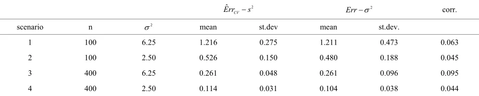
results a shown in Table 3. It nicely shows at the systematic error decreases mono- tonically from scenario 1 to scenario 4.
Means are very similar but standard
e CV estimates are much smaller. CV somehow shrinks the estimate of the systematic error towards the mean. The table shows that the correlations between the esti-
mate ˆ 2
CV
Err s and the true value Err2 are still
very low. The warning issued in Section 4 of [2] still holds. It is nearly impossible to estimate the prediction error of a particular regression model. Cross-validation is of very little help in estimating the actual error. It can only estimate the mean error, averaged over all potential
“training sets”. However, it might be helpful in selecting procedures that reduce the prediction error.
Finally, it should be pointed out that the cross-vali- dation results are in close agreement with the model based estimates of the prediction error as discussed in the same section of [2].
4. Cross-Validation Based Shrinkage
without Selection
4.1. Global Shrinkage
As argued by [2,11], the predictive performance of the resulting model can be improved by shrinkage of the model towards the mean. This gives the predictor
1ˆ
Y y c X x b
0 c 1
with shrinkage factor c, . In the following c will be called global shrinkage factor. Under the assumption of homo-skedasticity, the optimal value for c can be estimated as
2 heur
exp
ˆ 1 p s
c
SS
SS 2
with exp the explained sum of squares, s the esti-
mate of the residual variance and p the number of pre- dictors.
A model free estimator can be obtained by means of cross-validation. Let y i,xi,b1, i be obtained in the
cross-validation subset, in which observation i is not included, then can be estimated by minimizing c
21, 1
n
i i i i i
i
y y c x x b
[image:4.595.56.539.508.604.2]
Table 2. Simulation results for Errˆ CV and Err and their correlation (corr.) in models without selection.
ˆ CV
Err Err corr.
scenario n 2 mean st.dev mean st.dev.
1 1 00 6.25 7.470 1.160 7.461 0.473 0.024
2 100 2.50 3.029 0.474 2.980 0.188 0.029
3 400 6.25 6.505 0.470 6.511 0.096 -0.009
4 400 2.50 2.611 0.189 2.604 0.038 0.002
Table 3. Simulation results for Errˆ CVs
2 and Err2 and their correlation (corr.) in models without selection.
2
ˆ CV
Err s Err2 corr.
scenario n 2 mean st.dev mean st.dev.
1 1 00 6.25 1.216 0.275 1.211 0.473 0.063
2 100 2.50 0.526 0.150 0.480 0.188 0.045
3 400 6.25 0.261 0.048 0.261 0.096 0.095
[image:4.595.58.538.638.735.2]resulting in
1, 2 1, .i i i
i i x b b ng 1 1 ˆ n i i i cal n i i
y y x c x x
This estimate can be obtained by regressi yiy i
on
rcept. Islightly from ˆ
y as proposed in
u
1,
i i i
x x b in a model without an inte t
diff the one obtained by regressing yi
on [2]. The definition allows k-fold
ers
i
cross-validation and is not restricted to leave-one-o t cross-validation. The results of application of global shrinkage in the simulation data, ignoring the restriction
0 c 1, are shown in Table 4. Actually, c0 was never observed and c1 only occasionally.
ble shows that global shrinkage ca lp to
reduce the predictio r if the amount of in
Th n he
n erro formation
in
between reduction in predictio age and the predictio
ar
0 an ely. The
−0 10 for 9. The panel the
actual (true) prediction error based on our knowledge of
8, 0.05
e ta
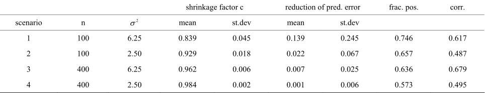
the data is low. For scenario 1 the mean of the shrink- age factor is 0.84 and the mean reduction of prediction error is 0.14. Corresponding values for scenario 4 are 0.98 and 0.001. For the latter all shrinkage factors are close to one and predictors with and without shrinkage are nearly identical. However, the positive correlation between the shrinkage factor c and the reduction in prediction error is counter-intuitive. To get more insight the data for scenario 1 with a small amount of infor- mation
n100,26.25
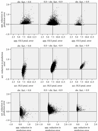
is shown in Figure 1.The re n error due
to shrink n error of the OLS models
lation
e shown for three categories of the shrinkage factor c, namely
c0.8 , 0.8
c 0.9
and
c0.9
. The frequencies of these categories among the 10,000 simu-lations ar espectiv upper
panel shows the apparent (estimated) prediction errors based on cross-validation and the apparent reduction achi- eved by global shrinkage. The differences between the three categories are small, but they are in line with the intuition that the largest reduction is achieved when the shrinkage factor is small. The quartiles (25%, 50%, 75%) of the apparent reduction are 0.09, 0.15, 0.27 for
0.8, 0.01,0.04,0.15
c for 0.8 c 0.9 and −0.07,
e 1754, 774 d 506, r
.02, 0 c0. middle shows
the true model. Here, the picture is completely different. Reduction of the prediction error only occurs when the shrinkage factor is close to one and the OLS prediction error is large. Substantial shrinkage with c0.8 tends to increase the prediction error. The quartiles of the true reduction are −0.29, −0.13, 0.04 for c < 0. , 0.18, 0.31 for 0.8 c 0.9 and 0.19, 0.28, 0.38 for c0.9. The lower panel shows the relation between the apparent
and the a ion. At first sight the res r
counter-intuitive. This phenomenon is extensively dis- cussed in [9]. What happens could be understood from the heuristic shrinkage factor
ctual reduct ults ou
2
heur exp
ˆ 1
c p s SS . If
b is “large” by random fluctuation, th
plained sum of squares SSexp heur ays
ose to 1 and does not “push” b in the direction of the true
e observed ex- is large and cˆ st cl
. If b is “small” andom fluctuati SSexp
is small and cˆheur will be close to 0 and might “push” in the wrong direction. This explains the overall neg
correlation r 0.253
by r on,
r
ative
ible to pred
se Shrinkage
rinkage factor, coin- PWSF), to be defined between apparent and actual re- duction of the prediction error. It must be concluded that
it is imposs ict from the data whether shrink-
age will be helpful for a particular data set or not. The chances are given under “frac. pos.” in Table 4. They are quite high in noisy data, but that gives no guarantee for a particular data set.
4.2. Parameterwi
[4] suggested a covariate specific sh ed parameterwise shrinkage factor ( as
ˆ
Y y X x c b 1 .
Here, c is a vector of shrinkag actors with
0 c 1
e f
for j 1, ,p
Λ
ultiplication:
and “” stands for coordi- nate-wise m
c b 1
jc bj 1,j. This way ofof Breiman’s Garrote [12]. See
also [9,13]. Sauerbrei sug arameterwise
shrinkage after model selection and to estimate the vector
c by cross-validation. As for the global shrinkage
(compared with OLS) achieved by global shrinkage in
regulation is in the spirit
gests to use the p
Tab mulation resu the reductio error
[image:5.595.57.539.643.736.2]out selection; “frac. pos.” stands for the fraction with positive reduction, “corr.” stand for the correlation lts for n in prediction le 4. Si
odels with m
between the shrinkage factor and the reduction.
shrinkage factor c reduction of pred. error frac. pos. corr.
scenario n 2 mean st.dev mean st.dev
1 100 6.25 0.839 0.045 0.139 0.245 0.746 0.617
2 100 2.50 0.929 0.018 0.022 0.067 0.657 0.487
3 400 6.25 0.962 0.006 0.007 0.025 0.636 0.679
Figure 1. Reduction of prediction error achieved by global shrinkage for different categories of the shrinkage factor c; data from scenario 1
n100,26 25.
. The upper panel shows the apparent prediction errors obtain d through cross- e validation, the middle panel shows the actual (true) prediction errors and the lower panel shows the relation between the apparent and the actual reduction.this could be obtained by regression without intercept f
o yiy i on
i i
1, i .e shrink as applied in the simulation data in
m
ith the
in scenario 1. In scenario 4 the in-
mated prediction error obtained from the cross-validation fit is far t
x x b
crease is moderate, but still present. Moreover, the esti-
Although this is against the advice of [4] parameter-
wis age w
odels without selection, ignoring the restrictions 0cj 1 for j1, ,Λ p. A summary of the results is given in Table 5.
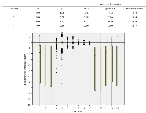
Using PWSF the average prediction error increases
when compared w OLS predictor. The increase is
large (about 10%)
oo optimistic. (Data not shown). The explana- tion is that parameterwise shrinkage is not able to handle the redundant covariates with no effect at all. This can be seen from the box plots in Figure 2.
Table 5. Comparison of the prediction errors of OLS, global se
mean prediction error
shrinkage and parameterwise shrinkage in models without lection.
scenario n 2 OLS global shr. parameterwise shr.
1 100 6.25 7.46 7.32 8.10 2 100 2.50 2.98 2.96 3.24
400 6.25
3 6.51 6.50 6.94
[image:7.595.51.536.106.480.2]4 400 2.50 2.60 2.60 2.77
Figure 2. Box plot of parameterwise shrinkage factors in models without selection. Results from scenario 4.
in models with many predictors without selection on stronger predictors parameterwise shrinkage cannot be recomm
rinkage values will be set to zero, but altogether such a
0.1573, 0.05
ended. The behavior is a bit better if negative sh
constraint is not sufficient. This is completely in line with Sauerbrei’s original suggestion.
5. Model Selection
Following [10] models are selected by backward eli-
mination at significance levels of
and 0.01. An impr selected is, shown in Fig
ession of which cova
ure 3.
riates are
ed, Type I and Type II
selec- he s,
the ones that have an influence on the outcome in the full model. In the simulation those ar the covariates
5.1. Number of Variables Select Error
The “softest” definition of model selection is the tion of covariates to be used in further research. T “optimal” model contains only the important covariate
e
4, , 10
X ΛX . If these are selected the other ones are
redundant. However if one of the important covariates is not selected, other non-important covariates can come to the rescue if they are correlated with the non-selected important covariate(s). In the simulation data non-im- portant covariates that can play such a role are covariates
1, 2, 13, 14
X X X X as can be seen from Table 1. The effect of omitting important covariates is the loss of explained variatio in the optimal model after selection or, equi- valently, the introduction of additional random error. If no selection takes place there is no loss of explained variation, but there is a large number of non-important covariates, leading to larger estimation errors. Even more important is a severe loss in general usability of such pre-
d nsider, for example, a prognostic model
comprising many variables. All constituent variables would have to be measured in an identical or at least in a
n
Figure 3. Frequency of selection per covariate.
similar way, even when their effects were very small. Such a model is impractical, therefore “not clinically useful” and likely to be “quickly forgotten” [14].
From Figure 3 we learn that in the
lot of information (scenario 4) all important variables
% easy situation with a
are selected in nearly all replications. For the 8 variables without an influence selection frequencies agree closely to the nominal significance level. For 15.73 se- lection frequencies are between 15.7% and 19.0%. The corresponding relative frequencies are between 5.1% and
6.55% for 5% and between 0.9% and 3.3% for
1%
. Results are much worse for situations with less
information. For the most extreme scen ob-
vious that all selected models deviate substantially from
the true model. For 1%
ario 1 it is
selection frequencies are
only between 23 and 25.1% for the 4 relevant vari-
4 7
.4%
ables X X with a weak effect. Even for
15.73%
these frequencies are only between 46.1%
and 57.3%. Of these X4 has the lowest frequency,
which is probably cau the strong correlation with
8
sed by
X . With 28.9% X1 has the largest frequency of se-
lection non-important covariates. That is
its strong correlation with X5. In 19.4% of
the simulations X1 is selected while the important vari- able X5 is not selected.
he effect of sel ion at the three levels is shown in
Figures 4-6.
Figure 4 summarizes the number of included variables for the different scenarios. In the simple scenario 4 all seven relevant variables
among d by
the
T ect
were nearly always selected. In ad
ment to the significance level. In 87.7% the correct
model was selected for 0.01
explaine
whereas redundant
variables without influence were ded when using
dition irrelevant variables were selected in close agree-
ad 0.157
For scenarios with less information the num-
ber of selected variables is usually smaller and the sig- l has a stronger influence on the inclusion fr
res 5
riates with nificance leve
equencies. Strong predictors are still selected in most of the replications, but the rest of the selected model does hardly ever agree to the true model. For each of the vari- ables with a weaker effect the power for variable inclu- sion is low.
The comparison of Figu and 6 nicely shows the balance between allowing redundant covariates (cova-
out effect in the selected model) and allowing loss of explained variation. The number of redundant covariates shown in Figure 5, corresponds directly to the type I error. It hardly depends on the residual variance
2
and the sample size n. Despite of some stronger correlations in our design the distribution is very close to binomial
8,
. The type II error is reflected by the loss of the variance of the optimal linear predictor
var X , or ,equivalently, the increase in residual variance 2, caused by not selecting all important cova-
riates. It could be translated into a loss of R2 by divi-
ding it by the marginal variance
2var Y var X , which is equal to 12.5 in sce-
n ios 1 and 3 (σ2 = 6.25) and 8.75 in scenarios 2 and 4
(σ2 = 2.5). This is shown in Figure 6.
General s aking, loss of R2 depends on both the
significance level used in the selection process and the ar
Figure 4. Number of included covariates.
Figure 5. Number of redundant covariates.
amount of information in the data reflected by residual
variance 2 and the sample size n. In scenario 4 with coefficient is 0.7) if the latter is not selected. That is shown in Table 6 for scenario 2 and 0.05
a high amount of information, the loss of R2 is
negligible and the nu er of redu variates can be
controlled by taking 0.01
. It has to
be kept in mind that other variables are also deleted making a direct comparison difficu . Concerning these two variables the correct model includes X5 and excludes
e in 69% of the replications. Here the
mb ndant co
. In sce ario 1 there is a
if the selec n tion
substantial loss of R2 is too strict and
0.1573
might be more appropriate.
As mentioned above and seen in Table 1 the variable
1
X can pa ly take over the role of rt X5 (correlation
lt
X1, which is the cas
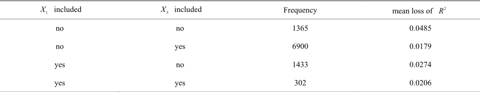
Figure 6. Loss of R in comparison to the full model. The bars show mean ± 1 st.dev. in the population of replications. Table 6. Inclusion frequencies and ave age loss of
2
R X X
r 2 for combinations of
1 and 5 for scenario 2 and 0 05. .
1
X included X5 included Frequency mean loss of R2
no no 1365 0.0485
no yes 6900 0.0179
yes no 1433 0.0274
[image:10.595.57.538.643.736.2]caused by ex f X5 substantially.
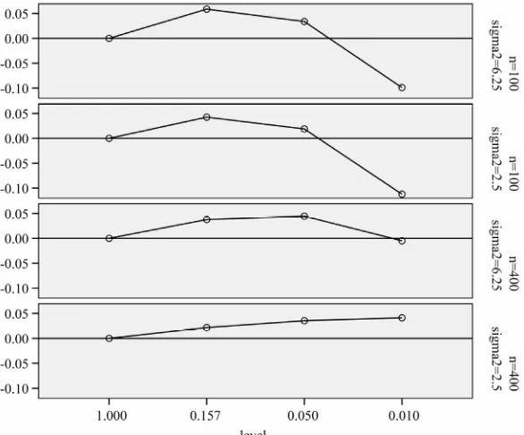
5.2. Assessment of Prediction Error
The predictio ror of a particular model d nds on the number of re ant covariates and the los explained variation. The average reduction of prediction error when
compared with no selection (significance le 1
clusion o
n er epe
dund s of
vel ) is uld be best com- he prediction
2
shown in Figure 7. Those numbers co pared with the systematic component of t error, Err , as reported in Table 3.
It nicely shows that the optimal level depends on the amount of information in the data. It also shows that moderate selection at 0.1573, in a univariate situ- ation equivalent with AIC or Mallows’ CP, can do very little harm. Even 0.05 gives always bette ults than no selection. For a small sample size the relative reduction in prediction error is small. For the large sample size elimination of several variab
r res
[image:11.595.152.445.462.705.2]les reduces the relative prediction error substantially for 0.05. The average number of selected variables is 7.02 for scenario 3 and 7.40 for scenario 4
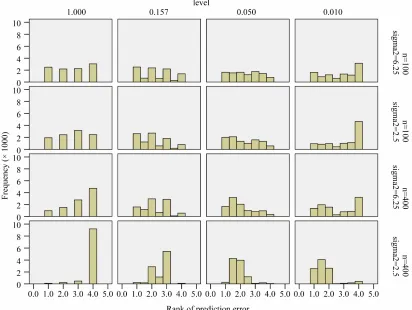
Figure 8 shows the prediction error ranking of the different levels in the ividual simulation data sets. Mean ranks were used in replications where the same model was selected. As observed before, the variation is very big and there is no outspoken winner, but there are some outspoken losers. In all scenarios it is bad not to select at all. However, for a small sample size it is even worse to use a very small s
.
ind
election level.
The p errors of the se els can be
estimated by cross-validation in such a way that in each cross-validation data set the whole sele rocedure is carried ou in Section 3 this will yield a correct esti- mate of the average prediction. Thus, it could be used to
select the al” significance level eral, but it
will not necessarily yield the best proc or the act- ual data set at hand.
s 7 and 9 shows that cross-valida- bout the re- le to notice
rediction lected mod
ction p t. As
“optim in gen
edure f
6. Post-Selection Cross-Validation
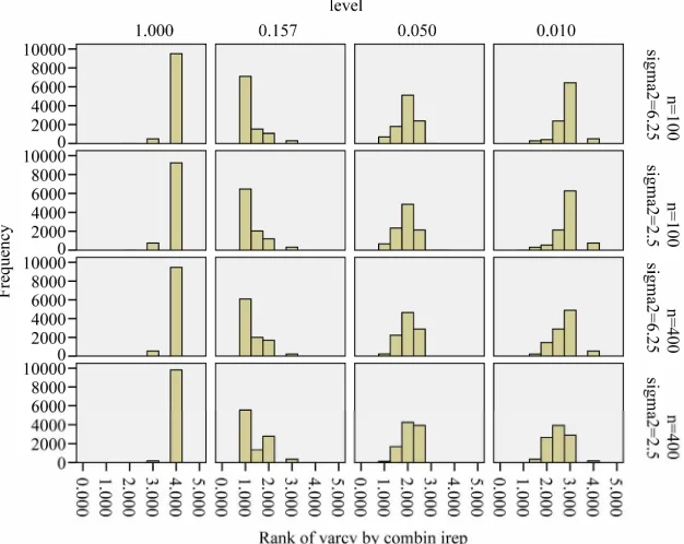
A common error in model selection is to use cross- validation after selection to estimate the prediction error and to select the best procedure. As pointed out by [15], this is a bad thing to do. That is exemplified by Figures 9
and 10.
Comparing Figure
tion after selection is far too optimistic a duction of the prediction error and is not ab
the poor performance of selection at 0.01 for the scenarios 1 and 2. Moreover, as can be seen from Figure 10, post-selection cross-validation tends to favor selec- tion at 0.1573 for all scenarios. This is no surprise because in univariate selection 0.1573 is equi- valent with using AIC, which is very close to using cross-validated prediction error if the normal model holds true.
6.1. Post-Selection Shrinkage
While cross-validation after selection is not able to select
re 7. Mean reduction prediction error as reported in Tables 2 and 3 for different α-levels. Values of Err−s2
21, 0.48, 0. ios 1-4, respectively (see Table 3). Figu
are 1.
Figure 8. Ranks of prediction error for different levels; rank = 1 is best, rank = 4 is worst.
[image:12.595.127.467.426.706.2]Figure 10. Ranks of estimated prediction error obtained from post-selection cross-validation for different levels; rank = 1 is best, rank = 4 is worst. The ranks of the true prediction error are shown in Figure 8.
cross-validation based shrinkage after selection can help to improve the model. The results are shown in Figure 11.
On the average, parameterwise shrinkage gives better predictions than global shrinkage, when applied after selection. An intuitive explanation is that small effects that just survive the selection, are more prone to selection bias and, therefore, can profit from shrinkage. In contrast, selection bias plays no role for large effects and shrink- age is not needed, see [16] and chapter 2 of [8]. Whereas global shrinkage “averages” over all effects, parameter- wise shrinkage aims to shrink according to these indi- vidual needs.
This can also be investigated by looking into the mean
squared
the best model, it might be of interest to see whether
estimation errors ˆjopt j, 2 of the regres-
sion coefficients conditional on the selection of cova- riates in the model. The c efficients o opt j, are the op-
timal regression coef in the selected model. As
discussed in ,j
ficients 2 the opt
Section coefficients can differ
from the j coefficients if there is correlation between
ce the effect of redundant covariates that only enter
that distinction. The precise mechanism is not quite clear yet. To get some better feeling what is going on, the observed scatterplot of parameterwise shrinkage factors versus the OLS estimator are shown in Figure 13 for covariate X3 (no effect), X6 (weak effect) and X9 (strong effect). These covariates are selected because the optimal parameter value when selected does not depend on which other covariates are selected as well. X3 is independent of all other variables and the other two variables are only correlated with one variable without influence. Therefore parameter estimates are theoretically equal to the true value in the full model. If the optimal value varies with the selection the graphs are a bit harder to interpret.
For X3, the covariate without effect and no correlation, the inclusion frequency is close to the type I error and in about half of these cases parameter estimates are positive and negative. The variable is selected in replications in which the estimated regression coefficient is by chance most heavily overestimated (in absolute terms) compared to the true (null) effect. One would hope that PWFS would correct these chance inclusions by a rule like “the
by chance, while the global shrinkage is not able to make
the covariates. Figure 12 shows the mean squared errors of the shrinkage based estimators relative to the mean quared errors of the OLS estimators for sample size
larger the absolute effect b , the smaller the shrinkage factor c”. Although most shrinkage factors are muc lower than one, Fig
h
ure 13 shows a different cloud: “the la
s
rger b , the larger c”.
A similar observation transfers to the plot for X9, which is selected in all replications. Therefore, selection bias is no issue for this covariate. The hope is that PWSF would move the estimate close to the true value β = 1.0. 100
n , scenarios 1 and 2 . Sample size n400 is not shown, because post-selection shrinkage has hardly any effect.
Figure 11. Reduction in prediction error obtained through s
deviation. hr kage after selection. Error bars show mean ± 1 standard in
Figure 12. Relative mean squared estimation errors of the partial regression coefficient per covariate (compared to OLS in the selected model) for the parameter estimates obtained by global (black) or parameterwise post-selection shrinkage (grey). Covariates 1-3 and 11-15 have no effect in the full model.
h b. Most values are close to 1, indicating that servation can be made for the cases where the correlated Generally speaking that does not happen: c increases
slowly wit
[image:14.595.146.453.420.658.2]Figure 13. Parameterwise shrinkage factors versus OLS estimates from selected models for covariates 3, 6 and 9; α = 0:05 and scenario 2; reference lines refer to the true value of the parameter.
variable X13 is included (plot not shown). X13 has no effect and the selection frequency (5.9%) agrees well to the type I error. If X13 is included, the shrinkage factor for X9 show a decreasing trend with c-values clearly below 1 if the estimate overestimates the true value
1 b
, and values around 1 if b1. One might say
that param rin helps to correct for chance
inclusions of ut r estimation errors.
X6 is a covariate with a weak effect. It is not included
in 19% of the replications, certainly cases in which the ue effect was underestimated by chance. The overall for the case where it is included shows a stronger increasing trend (compared with X9) tending to a value of about c0.96, if b is large. Here, X2 plays the role of a nfounding redundant covariate. In cases where it is included (plot not shown), the shrinkage factor for X6 is rather stable with median value about c0.88.
Some understanding obtained by the observa-
tion in [2] that in univariate he optimal shrinkage factor is given by
c
es eter sh
X13 b kag not fo
tr picture
co
can be models t
ˆ 21 var
cuni . If is small,
hard to esti ate. If
this quantity is very m is large it
could be estimated by 1 1 2
uni
c t . The parameter-
wise shrinkage factor behaves very similarly. This could
be seen from plotting PWSF against t (Graphs not
shown). Such a plot clearly shows that
ˆ
2
t (for
0.05
) is the cut-point for an inclusion and that
PWSF tends to increase with t for included variables. For large absolute t-values, PWSF’s are close to one. whereas they drop to about 0.8 for t close to 2. The relation between PWSF and t is similar for all three covariates X9. The difference between the covariates is the size of the effect and correspondingly the range of t
after selection.
The conclusion so far is that coordinate-wise shrinkage is helpful after selection. However it is not clear how to select the significance level. In a real analysis, the level should be determined subjectively by the aim of the study [4]. In the following we will compare backwards elimination with a procedure like the LASSO, that com- bines selection, shrinkage and fine-tuning.
7. Comparison with LASSO
of the penalty parameter . Because LASSO is quite time-consuming it was only applied on the first 2000 data sets for eac com ination h b of n and 2. Figure 14
shows the distr butioi n of the cross-validation based
for each co The variation in the penalty para-
meter
mbination.
, even in the simple situation of scenario 4 is surprisingly large. There is some correlation with the estimated variance in the full model, but that does not explain the huge variation.
The next Figure 15 shows the inclusion frequencies
[image:16.595.135.461.159.418.2] [image:16.595.131.463.449.721.2]ation based λ’s for the different scenarios. Figure 14. LASSO: histogram of the cross-valid
for the different covariates. Relevant variables are nearly always included, but LASSO is not able to exclude redundant covariates if there is much signal in the other ones. For example, in scenario 4 inclusion frequencies are 52% for X3 and 54% for X15, the two uncorrelated
bles with uence. The probable reason is that
selection and shri ge are controlled by the same penal- m
varia
ty ter
out infl nka
[image:17.595.156.442.484.717.2]. The menon is also nicely illustrated by
Figure 16.
Finally, the question how the prediction error of LASSO compares with the models based on selection and shrinkage is answered by Figure 17.
The conclusion must be that LASSO is no panacea. Concerning prediction error, it seems to be OK for noisy data (scenarios 1 and 2), but it is beaten by variable selection followed by some form of shrinkage if the data are less noisy (scenario 4). Most likely, that is caused by the inclusion of two many variables without effect. Vari- able selection combined with parameterwise shrinkage performs quit well. The choice of a suitable significance level seems to depend on the amount of information in
eas 0.01
pheno
the data. Wher has the best performance in
scenari s
en these
o 4, thi arios. In
level seems to be too low in the other
cases selections with 0.157
sc or
0.05
ve better pre ormance. Using
post shrinkage sli ces the prediction
errors with an advantage for parameterwise shrinkage.
8. Examples
8.1. Ozone Data
For illustration, we consider one specific aspect of a
study on ozone effects on school children’s lung growth. The study was carried out from February 1996 to Octo- ber 1999 in Germany on 1101 school children in first and second primary school classes (6 - 8 years). For more details see [17]. As in [18] we use a subpopulation of 496 children and 24 variables. None of the continuous vari- ables exhibited a strong non-linear effect, allowing to assume a linear effect for continuous variables in our analyses.
First, the whole data set is analyzed using backward elimination in combination with global and parameter- wise shrinkage and LASSO. Selected variables with cor- responding parameter estimates are given in Table 7 and mean squared prediction errors are shown in Table 8. The t-values are only given for the full model to illustrate the relation between the t-value and the parameterwise shrinkage factor. For variables with very large
ha selection
diction perf ghtly redu
t -values, PWSF are close to 1. In contrast, PWSFs are all over the place if t is small, a good indication that variables should be eliminated.
Mean squared prediction errors for the full model and the BE models were obtained through double cross-va- s-validated pre- ined by cross- validation within the cross-validation training set. Pre- diction error for the LASSO is based on single cross- validation because double cross-validation turned out to be too time-consuming. Therefore, the LASSO predic- tion error might be too optimistic.
MSE is very similar for all models, irrespective of applying shrinkage or not (range 0.449 - 0.475; the full model with PWSF is the only exception), but the number lidation in the sense that for each cros
diction, the shrinkage factors were determ
covar
Figure 17. Average prediction errors for different strategies.
Table 7. Analysis of full ozone data set using standardized covariates. The unadjusted R2 equals 0.67 in the full model and
drops only slightly to 0.64 for the BE(0.01) model. For the LASSO model it is 0.66.
method full model BE(0.1573) BE(0.05) BE(0.01) LASSO
cglobal 0.973 0.9876 0.9927 0.9958 −
variables b |t| cpar b cpar b cpar b cpar b
ALTER 0.016 1.42 1.09 0.015
ADHEU −0.010 0.90 1.03 −0.005
SEX −0.099 10.04 1.00 −0.101 0.98 −0.098 0.99 −0.096 0.99 −0.094 HOCHOZON −0.033 2.52 0.78 −0.036 0.64 −0.026 0.72 −0.014
AMATOP −0.002 0.15 −33.9
AVATOP −0.007 0.70 −0.20 −0.003
ADEKZ 0.004 0.38 −8.93
ARAUCH 0.003 0.31 −9.15
AGEBGEW 0.010 0.97 −0.00 0.007
FSNIGHT 0.008 0.77 −1.09 0.004
FLGROSS 0.173 11.42 0.97 0.181 1.01 0.181 1.01 0.184 1.01 0.172
FMILB −0.021 1.56 0.45 −0.018 0.64 −0.011
FNOH24 −0.036 2.85 0.72 −0.038 0.72 −0.032 0.79 −0.020
FTIER −0.004 0.37 −5.60 −0.002
FPOLL −0.026 1.32 −1.13 −0.020 0.79 −0.025 0.80 −0.011 FLTOTMED −0.019 1.93 0.86 −0.020 0.63 −0.012
FTEH24 −0.030 1.53 0.36 −0.032 0.25 −0.002
FSATEM 0.023 1.88 1.08 0.023 0.76 0.019
FSAUGE 0.003 0.30 −6.61
FLGEW 0.086 6.04 1.16 0.090 0.98 0.090 0.98 0.090 0.97 0.086 FSPFEI 0.027 2.20 0.68 0.027 0.87 0.032 0.89 0.026 0.90 0.019
FSHLAUF −0.008 0.75 −1.16
FO3H24 0.033 1.58 0.46 0.038 0.22
[image:18.595.60.538.467.738.2]Table 8. Mean squared prediction errors.
model no shrinkage global shrinkage parameterwise shrinkage full 0.0461 0.0461 0.0629
BE(0.1573) 0.0449 0.0449 0.0456
BE(0.05) 0.0475 0.0475 0.0470
BE(0.01) 0.0465 0.0465 0.0464
LASSO 0.0458
of variables in the model is very different. BE(0.01) selects a model with 4 variables, corresponding PWSF are all close to 1. Three variables are added if 0.05 is used as significance level. Using 0.157 selects a model with 12 variables. Two of them have a very low (below 0.3) PWSF, indicating that these variables may better be excluded. LASSO selects a complex model with 17 vari- ables.
Although they carry relevant information the double cross-validation results for the full data set lack the in- tuitive appeal of the split-sample approach. To get closer to that intuition the following “dynamic” analysis scheme is applied. First the data are sorted randomly, next the first ntrain observations are used to derive a prediction
model which is used to predict the remaining n n train
observations. This is done for ntrain 150, 200, 250,
300, 350 and repeated 100 time way an im-
pression is obtained how the different approaches behave with growing information. T
raphs. Figure 18 shows the mean number of covariates
proc are substanti train = 350 LA
selects on average 14.4 vari whereas BE(0.01)
lect .0 varia s. Figure 19 sho the evo tion
of t hri o r mo selected
BE( is alw oun 8 and BE(0
v 0 0.9 r ll m e
glo age s mu wer, from 83
with an increase to 0.95. Figure 20 s the mean
squ dictio f e di
W tion F ha ery nce,
wh glob nkag tor c ghtly reduce
MS dicti oves d if
vari ection rform and all E
than glob ge or. T ost im t
con that “BE(0.01 lowe PW
L ve ilar ction E’s, e
LASSO has to include many e cov es to
that.
8.2 at D
In a exam e wil strate e issues in a
stu ne d ng v le. T ta w
analysed in [19] and later used in many papers. 13 continuous covariates (age, weight, height and 10 body circumference measurements) are available as predictors for percentage of body fat. As in the book of [8] we excluded case 39 from the analysis. The data are avail- able on the website of the book. In Table 9 we give mean squared prediction errors for several models and shrink- age approaches. Furthermore we give these estimates for variables excluding X6, the dominating predictor. This
analysis assumes that X6 would not have been mea-
sured or that it would not have been publicly available. A related analysis is presented in chapter 2.7 of [8] with the aim to illustrate the influence of a dominating predictor and to raise the issue about the term “full model” and whether a full model approach has advantageous pro- perties compared with variable selection procedures. Using all variable MSEs of the models are very similar with a range from 18.76 - 20.80. Excluding 6
= 100, s. In that
X leads to erences between models are still negligible (25.87 - 27.47); with the full model
of the ozone data. For BE(0.157),
E(0.01) a SO we giv ter est
Table 10.
Exclud 6
a severe increase, but diff he results are shown in
g
included. More variables are included with increasing sample size (larger power) and differences between the
followed by PWSF as an exception. This agrees well with the results
edures al. For n SSO
ables, se-
s only 4 ble ws lu
he global s nkage fact r. Fo dels with
0.01) it ays ar d 0.9 for .157) it
aries between .96 and 8, but fo the fu odel th
bal shrink factor i ch lo starting 0.
show
ared pre n errors or th fferent strategies.
ithout selec PWS s a v bad performa
ereas the al shri e fac an sli
E of pre on. PWSF impr the pre ictor
able sel is pe ed has sm er MS
using a al shrinka fact he m portan
clusion is ) fol d by SF” and
ASSO have ry sim predi MS but th
mor ariat achieve
. Body F ata
second ple w l illu som
dy with o ominati ariab he da ere first
B nd LAS e parame imates in
ing X lts in the inclus of othe
bles for all approaches. As the ozone data O
rdly b is er
n fr (0.0 llow PW PWS
ariables selected b BE(0.01) are close to 1, whereas
ariables elected ditionall by BE .157) e
WSF va es below 0.9 and s metimes round 0.6. This
xample confirms that BE(0 1) followed by F
ives sim ar prediction MS but includes ch
aller er of bles
Dis
n and Conclusions
ildin able regression odel is a challenging task
a larger number of candid predictors is a e.
ving a situation with about to 30 variables in ind
full model is often unsu e of
iable selection is required bviousl subjec
nowledg has to play a key role in model buildin , but
en it is limited [ and d iven el-bu is
uired pite e c in t eratu 0,
resu ion r
vari-a in LASS
ha eli inates any m varia le, but the MSE ed by
not bett
tha om BE 1) fo S . F F of all
v y
v s ad y (0 all hav
P lu o a
e .0 PWS
g il E’s, a mu
sm numb varia .
9.
cussio
Bu g a suit m
if ate vailabl
Ha 10 m
the itable and som type
var . O y t matter
k e g
oft 20] ata-dr mod ilding
included under different strategies. Figure 18. Mean number of covariates
Figure 19. Evolution of the global shrinkage factor for differ BE(0.157) and BE(1.000) = “No selection”.
21] w
en
e consider backward elimination as a suitable approach, provided the sample size is not too small and
sensibly chosen according to the
t selection levels. From top to bottom BE(0.010), BE(0.050),
selected regression models.
In a simulation study and two examples we discuss the value of cross-validation, assess a global and a para- meterwise cross-validation shrinkage approach, both without and with variable selection, and compare results with the LASSO procedure which combines variable the significance level is
[image:20.595.135.465.366.622.2]Figure 20. Mean squared prediction error for the different strategies.
Table 9. Mean squared prediction errors.
model no shrinkage global shrinkage param.wise shrinkage
all no X6 all no X6 all no X6
full 19.05 26.74 19.04 26.71 20.59 31.47
BE(0.1573) 20.80 27.47 20.78 27.45 20.22 27.22
BE(0.05) 18.76 26.10 18.76 26.10 18.83 26.85 BE(0.01) 19.54 25.87 19.54 25.87 19.54 25.90
LASSO 19.08 26.22
selection with shrinkage [2,4,5]. As discussed in the introduction it is often necessary to derive a suitable explanatory model which means that the effects of indi- vidual variables are important. In this respect a sparse model has advantages, both from a statistical point of
direct effects of irrelevant variables if a relevant variable is not included. It seems consensus that stepwise and other variable selection procedures have limited value as tools for model building in small studies ([8,21] Section 2.3) and 10 observations per variable often considered
of n 100
view and from a clinical point of view. In a related con- text [22] refer to parameter sparsity and practical spars-
ty.
as a lower boundary to derive an explanatory model [23]. Based on this knowledge it is obvious that a sample size i
9.1. Design of Simulation Study
Our simulation design was used before for investigations of different issues [10]. We consider 15 covariates with seven of them having an effect on the outcome. In addi- tion, multicollinearity between variables introduces in-
is
(6.7 per variable) is low. As a more realistic 400
. Concerning the resi- du
scenario we also consider n
al variance we have chosen two scenarios resulting in
2 0.5
R and R20.71. The 4 scenarios reflect the
[image:21.595.56.537.453.553.2]Table 10. Parameter estimates for the standardized variables.
BE(0.1573) BE(0.01) LASSO
all no X6 all noX6 all no X6
var. b cpar b cpar b cpar b cpar b b
1
X 0.77 0.85 2.76 0.95 2.49 0.98 0.89 2.49
2
X 8.46 0.99 8.86 0.99 4.74
3
X −0.84 0.91 −2.90 0.99 −1.11 0.93 −2.99 0.99 −0.81 −2.17
4
X −0.76 0.69 −0.93 0.63 −0.80 −0.47
5
X −1.09 0.71 −0.76 1.56
6
X 8.93 0.96 8.01 0.99 8.54
7
X −0.57 1.41
8
X 1.01 0.71 0.54 0.99
9 X 10 X 0.18 11 X 0.40 12
X 0.73 0.59 0.43
13
X −1.58 0.98 −2.64 1.00 −1.57 0.97 −2.97 0.96 −1.64 −2.32
and therefore on the comparison between different proce- dures.
a Selection
The fin of Section 3 c
does imate the perfor e model at hand
but the erage perform e over all ble “training
sets”. T ults of Se confirm t
hrink-age o impro diction per nce in data
with little information [2,11] like in the first scenario
with 0 and . However, the results
show actual val f the global ge factor
ret [9] hrinkage is a bit counter-
9.2. Cross-Validation nd Shrinkage without
dings not est
onfirm that cross-validation mance of th
av anc possi
he res ction 4 hat global s
can help t ve pre forma
10
n 26.25
u o that th rd to e interp e . S shrinka is ha
intuitive. Considerable shrinkage is a sign that something is wrong and application of shrinkage might even in- crease the prediction error. That is evident from the nega- tive correlation 0.253 between apparent and actual reduction in prediction error in the simulations from scenario 1. For the more informative scenarios 2-4 all shrinkage factors are close to one and predictors with and without shrinkage are nearly identical. It must be con- cluded that it is impossible to predict from the data a particular data set
positive and negative signs and some of them have values far away from the intended range between 0 and 1.
ediction error is o com-
pare result rom variable selection proce es. This
plies that able predic th favorable statistical
in (or only rest of an is. In
rast to such a statistically analysis r chers
often the to derive a planato odel
willing to accept a m or
prediction per ance [6]. E ing relevant variables
2
erion fo
ous in st ith a lo
whether shrinkage will be helpful for or not.
Our results confirm that it does not make any sense to use parameterwise shrinkage in the full model [4]. Esti- mated shrinkage factors are not able to handle redundant covariates with no effect at all. Therefore they can have
9.3. Variable Selection and Post Selection Shrinkage
Most often pr the main criteria t
s f dur
im a suit tor wi
criteria are the ma ) inte analys
cont guided esear
have and are
aim suitable ex ry m
odel with slightly inferi xclud
form
results in a loss of R and the inclusion of variables without effect complicates the model unnecessarily and usually increases the variance of a predictor. We used several criteria to compare the full model and models derived by using backward elimination with several val- ues of the nominal significance level, the key criterion to determine complexity of a selected model, and the LASSO procedure. The number of variables is a key crit r the interpretability and the practical useful- ness of a predictor. BE(0.01) always selects the sparsest model, but such a low significance level may be danger-
udies w w amount of information. Our