Munich Personal RePEc Archive
Sectoral Labor Market Effects of Fiscal
Spending
Wesselbaum, Dennis
University of Hamburg, German Physical Society, EABCN
9 September 2014
Sectoral Labor Market Effects of Fiscal Spending
Dennis Wesselbaum
∗University of Hamburg, DPG, and EABCN
September 9, 2014
Abstract
This paper studies sectoral effects of fiscal spending. We estimate a New Keynesian model with search and matching frictions and two sectors. Fiscal spending is either wasteful (con-sumption) or productivity enhancing (investment). Using U.S. data we find significant differ-ences across sectors. Further, we show that government investment rather than consumption shocks are driver of fluctuations in sectoral and aggregate outputs and labor market variables. Finally, government investment shocks are much more effective in stimulating the economy than spending shocks. However, this comes at the cost of a very persistent increase in debt.
Keywords: Government Consumption, Government Investment, Search and Matching, Sec-toral Effects.
JEL codes: C11, E32, E62, H5.
∗University of Hamburg, Chair of Economics, Methods in Economics. Email:
1
Introduction
During the Great Recession governments around the world used fiscal policy measures to counter the large adverse effects on real activity. Consecutively, the effects of fiscal policy became a center of attraction in macroeconomic research. However, academic research related to the sectoral (labor market) effects of fiscal policy is rather sparse. This is surprising as e.g. the famous Bernstein and Romer (2009) report on the job market effects of the American Recovery and Reinvestment Act (ARRA, for short) breaks down job gains by Industry.
This paper closes this gap and analyzes the sectoral labor market effects of fiscal spending and, in particular, highlight the differences between government consumption and investment. We build a stylized New Keynesian model of the U.S. economy with search and matching frictions and two production sectors. One sector produces goods, while the other sector provides services. Monetary policy in this model follows a Taylor-type interest rate rule. Fiscal policy can use its resources (generated by lump-sum taxation) for government consumption or by building-up the government capital stock. While government consumption is wasteful and works mainly as a demand-side shock, government capital is used in the production process and affects marginal productivity. We want the reader to think about government capital as infrastructure which is an exogenous input into the production process. The importance of government investments can be inferred from the observation that roughly 30 percent of the 550 Billion U.S. Dollars in the ARRA was allocated to infrastructure programs. We then estimate this model on U.S. time series using Bayesian methods.
Several findings stand out. The manufacturing labor market is characterized by a larger steady state separation rate and a lower bargaining power compared to the service sector labor market. In contrast, vacancy posting costs are almost five times larger in the service sector than in the manufacturing sector. Further, government consumption and investment follow fiscal rule with feedback to output but not to government debt. Government consumption reacts roughly three times as much to variations in output than government investment.
A variance decomposition analysis shows that government investment plays a major role in driving aggregate and sectoral output and inflation. Since we abstract from private capital our results should be interpreted as an upper bound on the role of government investment. Employment appears to be driven by the sectoral technology shocks and, for the manufacturing sector, the aggregate technology shock. Monetary policy plays a minor role but seems to play a non-negligible role in explaining movements in service sector employment.
Fiscal spending shocks increase sectoral and aggregate output. Unemployment decreases on impact but increase in the medium-run. Sectoral differences are driven mainly by the differences in the wage setting, different vacancy posting costs, and different separation rates. Overall, we find that investment shocks create larger real effects than consumption shocks. However, they generate a large increase in government debt that only slowly converges back to the steady state.
Gertler et al. (2008), Lubik (2009), and Di Pace and Villa (2013) estimate search and matching models. While Lubik (2009) estimates a stylized version of the search and matching model, Di Pace and Villa (2013) use a richer model with capital and hours worked. Besides those papers there are studies estimating search and matching models for other countries. Lubik (forthcoming) estimates such a model for Hong Kong, Lin and Miyamoto (2012) use data for Japan, and Wesselbaum (forthcoming) focuses on Australia.
Second, we add to literature on sectoral effects of fiscal policy. However, the papers in this category interpret sectoral as the difference between traded vs. non-traded goods and perform their analysis in an open economy framework. Our analysis, in contrast, is performed in a closed economy setting. Bénetrix and Lane (2010) perform a VAR analysis for a number of European countries and find that government spending increases the relative size of the non-traded vis-a-vis the traded goods sector. They conclude that fiscal shocks do affect the sectoral allocation while having aggregate effects. Along this line, Monacelli and Perotti (2008) use a structural VAR and find a positive comovement in consumption and production for the manufacturing and the service sector in an open-economy model. They show that a canonical open-economy business cycle model fails to generate such a positive comovement.
Further, Bouakez et al. (2013) estimate SVARs for subcategories of government spending and investment. They find large differences in the effectiveness of fiscal policy across sectors. The largest effects are obtained for changes in government employment while spending has only limited effects on output.
Finally, our paper is related to the work by Obstbaum (2011), who builds a New Keynesian search and matching model with fiscal policy. However, the main difference to our paper is that fiscal spending is purely government consumption. One of the main findings is that the effects on labor market variables and output depends crucially on the financing scheme.
The paper is structured as follows. Section 2 develops our model and section 3 presents our data set and discusses our estimation results. Section 4 briefly concludes.
2
Model Derivation
We develop a discrete-time model for the U.S. economy with two different production sectors. This model is an extension to the model developed in Wesselbaum (2011), while labor market frictions follow the contributions from Mortensen and Pissarides (1994) and den Haan et al. (2000). Households maximize utility by setting the path of consumption, which is a CES aggregate of differentiated products. Firms set prices and choose employment in two sectors: manufacturing (i.e. goods production) and service and produce a final good using both sectoral outputs. We further assume that separations are endogenous and driven by job-specific productivity shocks. Hence, there is a flow of workers into unemployment while unemployment-employment transition is subject to search and matching frictions.
fiscal policy uses consumption and investment into government capital to spend resources.
2.1
Households
Our economy is populated by a family with two types of infinitely-lived workers. They inelastically supply one unit of labor and being represented by the unit interval. In addition, household members insure each other against income fluctuations as in Merz (1995). They have the following preferences over consumption
Et
∞
t=0
βt[ln (Ct)], (1)
where the conditional expectation operator is denoted by Et. Households discount the future with
a factorβ ∈(0,1). The intertemporal budget constraint faced by the family is
Ct+
Bt+1
Pt+1 =
WtxNt+Rt
Bt
Pt+1 +but+ Πt+Tt, (2)
where x ∈ m, s is the index for the worker’s sector, either m for manufacturing or s for service. Further, but is income from unemployment with b > 0 corresponding to unemployment benefits,
while Wx
tNt is labor income. Bond holding, Bt, pays a gross interest rate Rt, Πt are aggregate
profits and Tt are lump sum transfers from the government.
Then, the optimality condition for the household is a standard Euler equation given by
1
Ct
=βEt Rt Pt
Pt+1
1
Ct+1 . (3)
2.2
Labor Markets
The firm searches for workers on two discrete and closed markets. This assumption is based upon the limited ability of workers to switch sectors due to specific skills, initial education, and employment protection legislation (see e.g. Lamo et al. (2006)).1 One of those market contains all workers in
the manufacturing sector, and the other contains all workers in the service sector. This assumption allows us to account for differences in vacancy filling rates across sectors, found by Davis et al. (2009) and estimate sectoral matching functions.2
New matchesMtxare created from the pool of unemployedUtxand the number of open vacancies
Vx
t according to the matching function
M(Utx, Vtx) =mx(Utx)µ
x
(Vtx)1
−µx
, (4)
whereµx ∈(0,1)is the elasticity of the matching function with respect to unemployment and the match efficiency is governed bymx >0. Then, the probability of a vacancy being filled in the next
period is q(θx
t) = m(θxt)
−µ. Labor market tightness is given by θx
t = Vtx/Utx. Tightness is a key
variable in search and matching models as it generates a congestion externality: if a firm posts a
vacancy it decreases simultaneously the probability for other firms to fill a vacancy. On the other hand, an additional searcher causes negative search externalities for other searchers, i.e. reduces the job finding probability of all other searchers.
The firm’s exit site is characterized by endogenous separations. The total number of separations in each sector, at firm iis given byρx(˜axit) =F(˜axit), where ˜axit is the cut-off point of idiosyncratic
productivity andF(·)is a time-invariant distribution with positive supportf(·). Its mean is given by ωx and ςx is the dispersion of the function.
Connecting entry and exit site gives the evolution of employment at firmias
Nitx+1 = (1−ρxit+1)(Nitx+Vitxq(θxt)). (5)
The firm has two margins to control employment: either adjust the number of posted vacancies or set the critical threshold, which then influences the separation rate.
Finally, the aggregate values are defined by
Uitagg = Uitm+Uits, (6)
Mitagg = Mm
it +Mits, (7)
Vitagg = Vitm+Vits, (8)
θaggit =
Vitagg
Uitagg. (9)
2.3
Firms
Firms use a standard Cobb-Douglas production technology with elasticity0≤ϑ≤1
Yit=At(Yitm) ϑ
(Yits)1
−ϑ
, (10)
to produce the final production good Yit using the output produced in the manufacturing sector
Ym
it and the service sectorYits.
The sector-specific production technologies are
Yitx= Gkt αx
AxtNitx
˜
ax it
ax f(a
x)
1−F(˜ax it)
dax ≡ Gkt αx
AxtNitxH(˜axit), (11)
where we useH(˜axit) = ˜ax ita
x f(ax ) 1−F(˜ax
it)
dax to ease notation. Further,αx denotes the sector-specific
output elasticity w.r.t. government investment. The elasticity of government investment is a key factor in discussing its effectiveness. While aggregate productivityAtand sectoral productivitiesAxt
are common to all firms, the specific idiosyncratic productivityax
itis idiosyncratic and every period
it is drawn in advance of the production process from the corresponding distribution function. Further, we assume that government capital is used in the production of sectoral outputs as the final good production only acts as an aggregation of sectoral outputs.
We assume that all three technology shocks follow autoregressive processes
lnAt = ρAlnAt−1+eA,t, eA,t∼N(0, σA), (12)
where the error terms are i.i.d. and normally distributed.
The firm maximizes the present value of real profits given by
Πi0 =E0 ∞
t=0
βtλt λ0
Pit
PtYit
− Wm
it − Wits −cmVitm−csVits−
ψ
2
Pit
Pit−1
−π
2
Yt , (14)
while perfect capital markets imply that the firm discounts with the households subjective discount factor β. The first term in parenthesis is real revenue, the second and the third term is the wage
bill, which is given by the aggregate of individual wages
Witx=Nitx
˜
ax it
wtx(ax)
f(ax)
1−F(˜ax it)
dax. (15)
The wage is not identical for all workers, instead it depends on the idiosyncratic productivity across sectors. The fourth and fifth term reflect the total costs of posting a vacancy. The latter term corresponds to Rotemberg (1982) price adjustment costs. The degree of these costs is measured by the parameter ψ ≥ 0, while the costs are related to the deviation from steady state inflation, π.
The first-order conditions with respect to employment, vacancies, and prices are
ξxt = ϕtAxtH(˜axt)−
∂Wx t
∂Nx t
+Etβt+1(1−ρxt+1)ξxt+1, (16)
cx
q(θxt)
= Etβt+1(1−ρxt+1)ξxt+1, (17)
ǫ(1−ϕt) = 1−ψ(πt−π)πt+Etβt+1 ψ(πt+1−π)πt+1Yt+1
Yt .
(18)
The current period average value of workers is given by ξx
t and ϕt reflects real marginal costs.
Further,π denotes the steady state inflation rate. Combining (16) and (17) gives the job creation condition
cx q(θxt)
=Etβt+1(1−ρxt+1) ϕt+1Axt+1H(˜axt+1)−
∂Wx t+1
∂Nx t+1
+ c
x
q(θxt+1)
.
Hiring decisions are a trade-off between the cost of a vacancy and the expected return. The lower the probability of filling a vacancy, the longer the duration of existing contracts - as 1/q(θxt) is the
duration of the relationship between firm and worker - because the firm is not able to replace the worker instantaneously.
As an example, if expected productivity rises, the right-hand side rises while the left-hand side on impact remains unchanged. Higher expected revenue creates incentives for the firm to post more vacancies, which increases labor market tightness. Because the probability that an open vacancy is filled is decreasing in the degree of labor market tightness the cost of posting vacancies increases and reduces incentives to post new vacancies.
Finally, a log-linearization of the last first-order condition around a zero inflation steady state gives the New Keynesian Phillips curve
ˆ
πt=βEtπˆt+1+κϕˆt, (19)
2.4
Wage Determination
Firm and worker engage in individual Nash bargaining and maximize the Nash product
wxt =argmax (Etx− Utx)η(Jtx− Vt)1−η . (20)
The first term is the worker‘s surplus, the latter term is the firm‘s surplus and 0 ≤ η ≤1 is the exogenously determined, constant relative bargaining power. The worker’s threat point isUx
t, the
value of being unemployed and the firm’s threat points are given byVtwhich is zero in equilibrium due to a free entry condition. The asset value of a filled job for the firm isJx
t and for the worker, Ex
t, is the asset value of being employed.
Then, the solution to the problem is an optimality condition
Ex
t(axt)− Utx=
η
1−ηJ x
t (axt). (21)
To obtain an explicit expression for the individual real wage we have to determine the asset values and substitute them into the Nash bargaining solution. The three Bellman equations are given by
Jtx(axt) = ϕtAxtaxt −wxt(axt) +Etβt+1 (1−ρxt+1) ˜
ax t+1
Jtx+1(ax) f(a
x)
1−F(˜ax t+1)
dax , (22)
Ex
t(axt) = wxt(axt) +Etβt+1 (1−ρxt+1) ˜
ax t+1
Ex t+1(ax)
f(ax)
1−F(˜ax t+1)
dax+ρxt
+1Utx+1 , (23)
Utx = b+Etβt+1
θxtq(θxt)(1−ρxt+1) ˜ax t+1
Ex t+1
f(ax ) 1−F(˜ax
t+1)
dax
+(1−θx
tq(θxt)(1−ρxt+1))Utx+1
(24)
The first equation is the asset value of the job for the firm depending on the real revenue, the real wage and if the job is not destroyed, the discounted future value. Otherwise, the job is destroyed and hence has zero value. The second equation is the asset value of being employed for the worker and depends on real wage, the discounted continuation value, and in case of separation the value of being unemployed. The latter equation is the asset value of being unemployed. Unemployed worker receive unemployment benefits, the discounted continuation value of being unemployed, and if she is matched she receives the value of future employment. Finally, the expression for the wage is
wx
t(axt) =η(ϕtAxtaxt +cxθxt) + (1−η)b. (25)
The gap between the real wage and the reservation wage is increasing in every time-dependent component and the worker’s bargaining power.
At the end of this section we determine the cut-off point of idiosyncratic productivity. The firm will endogenously separate from a worker if and only if
Jtx(axt)<0, (26)
i.e. if the asset value of the worker for the firm is negative. Using this condition, the expressions for the real wage, and the vacancy posting condition in equilibrium yields the productivity threshold
˜
axt =
1 (1−η)ϕtAxt
(1−η)b+ηcxθxt −
cx
q(θxt)
2.5
Monetary and Fiscal Policy
The monetary authority targets the nominal interest rate by following a standard Taylor rule, given by
ˆ
Rt=φππˆt+φyYˆt+ert, (28)
where φπ > 0 and φy > 0 are the respective weights on inflation and output. Monetary policy
shockser
t follow an autoregressive processes
lnert =ρrlnert−1+er,t, er,t ∼N(0, σr), (29)
where the error terms are i.i.d. and normally distributed.
Fiscal policy finances expenditures with lump-sum taxes,Tt, and by issuing government bonds,
Bt,
Bt+1
Rt =Bt+G c
t+It−Tt. (30)
The government can uses its resources either for government consumption or for building up the government capital stock.
Government consumption is wasteful and follows a fiscal rule with feedback to output and government debt
Gct = −γcYt−λcBt+Gd,t, (31)
lnGd,t = ρGlnGd,t−1+eGc,t, eGc,t∼N(0, σG), (32)
whereGd,tare discretionary spending shocks with i.i.d. normally distributed errors. Here,γcgives
the weight of output andλcgives the weight of debt in the reaction function.
In contrast, government capital is used in the production process and follows
Gkt = (1−δ)Gtk−1+It−1, (33)
whereδ >0is the depreciation rate of the capital stock andIt−1 is the investment into new capital.
Here, we assume that there is a time-to-build lag following Kydland and Prescott (1982) and, more recently, Bouakez et al. (2014).3 Again, we use a fiscal rule with feedback to output and government
debt to model government investment
It = −γkYt−λkBt+Id,t, (34)
lnId,t = ρIlnId,t−1+eI,t, eI,t∼N(0, σI), (35)
where discretionary investment spending areId,t with i.i.d. normally distributed errors.
Finally, the resource constraint is given by
Yt=Ct+cmVitm+csVits+Gct+It+ψ
2 (πt−1)
2Y
t, (36)
such that the final output good can be consumed by the private and the public sector, used as vacancy posting costs in both sectors, or can be used to build up the government capital stock.
2.6
Calibration and Priors
We calibrate the model for the United States on a quarterly basis and present the prior choice for the estimated parameters.
Households discount the future with β= 0.99, and the demand elasticity is set to 11.
The unemployment rates are taken from BLS household data. For the manufacturing sector we take a value of 12 percent and for the service sector the unemployment rate is set to eight percent. For both sectors, we assume that the idiosyncratic productivities are log-normally distributed with zero mean and a variance of 0.12 as in Krause and Lubik (2007). The job filling rate in steady state is set to 0.7 in line with Krause and Lubik (2007). The steady state cut-off point for idiosyncratic productivity is given by a˜x = F−1(ρx). Then, matches in steady state are computed according
toMx = ρx
1−ρxNx, vacancies are given by Vx =Mx/qx, and labor market tightness is tightness is
θx =Vx/Ux. We can compute match efficiency asmx=qθµx
.
Government consumption is set to 25 percent of output and government investment is set to 5 percent of output in line with the values taken from the NIPA tables.
For the bargaining power of workers we assume a symmetric split and impose a normally distributed prior with mean 0.5 and standard deviation 0.05. Further, the parameter that drives the separation rates belongs to the beta family and has a mean of 0.1 and a standard deviation of 0.02. Vacancy posting costs are assumed to be gamma distributed with mean 0.05 - as usually assumed in the literature - with standard deviation 0.02. Finally, the elasticity of the matching function is assumed to be beta distributed with mean of 0.5 and standard deviation 0.05.
The parameter ϑ in the aggregate production function is assumed to be normally distributed with mean 0.5 and standard deviation 0.1. The sector-specific elasticities of government investment are both normally distributed with mean 0.05 and standard deviation 0.05. Price adjustment costs,
ψ, are assumed to be normal distributed with mean 40 and standard deviation 5, based upon the calibrated value by Krause and Lubik (2007).
The prior on the depreciation rate of government investment belongs to the beta family with mean 0.02 and standard deviation of 0.01. The prior is set to the usually assumed value for private capital in DSGE models. Then, we set the priors for the fiscal rule parameters. For the feedback to output and debt we assume prior belonging to the gamma family with mean 0.1 and standard deviation 0.1.
3
Estimation Results
3.1
Data
We use quarterly, seasonally adjusted time series for the United States from 1954:3 to 2013:4 (238 observations). Total output and the sectoral outputs are taken from the Bureau of Economic Analysis’ NIPA tables. Total output is gross domestic product (A191RC1) in billions of U.S. Dollars. Manufacturing output is the sum of durable (DDURRC1) and nondurable (DNDGRC1) goods. Government consumption is the sum of current expenditures (W013RC) and capital transfer payments (W020RC1) minus the consumption of fixed capital (A918RC1). Government investment is the sum of defense (A788RC1) and nondefense (A798RC1) gross investment plus state and local gross investment (A799RC1). All variables are divided by the personal consumption expenditures price deflator (DPCERG3), with basis year 2009.
Labor market variables are taken from the Bureau of Labor Statistics. Employment in the man-ufacturing sector is employment in the nondurable (CES3200000001) and durable (CES3100000001) sector. Employment in the service sector is the sum of employment in the private service-providing (CES080000001), professional and business service (CES6000000001), and other services (CES8000000001) sector.
Finally, the interest rate is the effective Federal funds rate taken from the St. Louis FED FRED system. Before we run our estimation, we write the time series in logarithmic scale and use a Hodrick-Prescott filter with λ = 1600to generate the cycle component. Then, we use 500.000
draws for our MCMC chains to obtain the estimation results.
3.2
Point Estimates
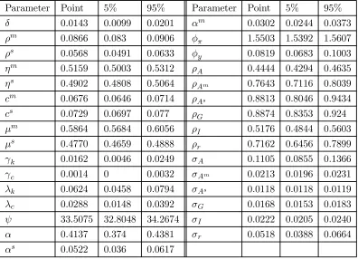
Table 1 presents the point estimates and the 95 percent confidence intervals for the set of estimated parameters.4
The separation rate in the manufacturing sector is larger compared to the service sector (0.09 vs. 0.06). They are sizably smaller compared to the value found by Lubik (2009) for the aggregate separation rate of 0.12. The elasticity of the matching function with respect to unemployment in the manufacturing sector is larger as in the service sector (0.59 vs. 0.48). The smaller value in the service sector implies that i) the finding rate reacts more elastically to changes in labour market tightness and ii) the matching rate is less sensitive to changes in labour market conditions. However, those values are smaller compared to the estimated value in Lubik (2009) of 0.74. We find that workers in the service sector have a slightly smaller bargaining power compared to the manufacturing sector (0.49 vs. 0.52). This implies a smalle share of the surplus in the service sector is allocated to the worker. Next, we consider the cost of posting a vacancy. We find that the cost of posting a vacancy is slightly larger in the service sector (0.073) than in the manufacturing sector (0.068). Usually, this parameter is calibrated at around 0.05 for standard (aggregate) matching models, which seems to be a reasonable value given our estimates. The price adjustment cost
Table 1: Posterior estimates.
Parameter Point 5% 95% Parameter Point 5% 95%
δ 0.0143 0.0099 0.0201 αm 0.0302 0.0244 0.0373
ρm 0.0866 0.083 0.0906 φ
π 1.5503 1.5392 1.5607
ρs 0.0568 0.0491 0.0633 φ
y 0.0819 0.0683 0.1003
ηm 0.5159 0.5003 0.5312 ρ
A 0.4444 0.4294 0.4635
ηs 0.4902 0.4808 0.5064 ρ
Am 0.7643 0.7116 0.8039
cm 0.0676 0.0646 0.0714 ρ
As 0.8813 0.8046 0.9434
cs 0.0729 0.0697 0.077 ρ
G 0.8874 0.8353 0.924
µm 0.5864 0.5684 0.6056 ρ
I 0.5176 0.4844 0.5603
µs 0.4770 0.4659 0.4888 ρ
r 0.7162 0.6456 0.7899
γk 0.0162 0.0046 0.0249 σA 0.1105 0.0855 0.1366
γc 0.0014 0 0.0032 σAm 0.0213 0.0196 0.0231
λk 0.0624 0.0458 0.0794 σAs 0.0118 0.0118 0.0119
λc 0.0288 0.0148 0.0392 σG 0.0168 0.0153 0.0183
ψ 33.5075 32.8048 34.2674 σI 0.0222 0.0205 0.0240
α 0.4137 0.374 0.4381 σr 0.0518 0.0388 0.0664
αs 0.0522 0.036 0.0617
parameter is estimated to be 33.5, which is slightly smaller compared to the calibrated value in Krause and Lubik (2007) which is set to match the Calvo probability of an average price duration of four quarters. Hence, prices are re-set more frequently.
The depreciation rate of government investment is estimated to be 0.0143 which, intuitively, is smaller compared to the depreciation of private capital usually assumed to be close to 0.025. The elasticity of aggregate production function, ϑ, is estimated to be 0.41. This implies a larger weight on service-sector output. The service-sector output elasticity w.r.t. government investment is estimated to be 0.05, which is larger as in the manufacturing sector (0.03). Our results imply that government investment is more productive in the service sector than in the manufacturing sector. In the literature, the elasticity of government investment varies between 0.24 (Aschauer (1989)) and negative values (Evans and Karras (1994)).
54 58 62 66 70 74 78 82 86 90 94 98 02 06 10 −0.1
−0.05 0 0.05
54 58 62 66 70 74 78 82 86 90 94 98 02 06 10 −0.4
−0.2 0 0.2 0.4 0.6 0.8
54 58 62 66 70 74 78 82 86 90 94 98 02 06 10 −0.05
0 0.05
Technology: Manufacturing Technology: Service
Monetary Policy Aggregate Technology
[image:13.595.175.434.85.295.2]Gov. Consumption Gov. Investment
Figure 1: Estimated shocks. Vertical axis presents quarters from 1954 to 2010.
We find that the sectoral technology shocks are highly autocorrelated in contrast to the ag-gregate technology shock. Further, we find that the government spending shock shows a larger degree of autocorrelation compared to the government investment shock. The autocorrelation of the monetary policy shock is midway between the two expenditure shocks.
Finally, we find similar values for the standard deviations of all shocks, with the aggregate technology shock and the monetary policy shock being the most volatile ones. Figure ??presents
the time series of the estimated shocks.In conclusion, we find evidence that sectors do behave significantly different. This holds for the exit as well for the entry side of job flows.
3.3
Shock Decomposition
In this section we want to highlight the main driving forces of business cycle fluctuations in key aggregate and sectoral variables. Figure?? presents the unconditional variance decomposition.
Our results show that output in both sectors is mainly driven by variations in aggregate tech-nology. Further, manufacturing sector output is to 40 percent driven by the manufacturing sector technology shock. In contrast, the service sector technology shock explains only about 30 percent of total variation in service sector output. Innovations in monetary policy are more important for service sector output than for output in the manufacturing sector output. Government expenditure shocks explain less than five percent of sectoral outputs.
Output: M Output: S Inflation Employment: M Employment: S 0
0.1 0.2 0.3 0.4 0.5 0.6 0.7 0.8 0.9 1
[image:14.595.125.492.84.293.2]Technology Technology: M Technology: S Monetary Policy G Consumption G Investment
Figure 2: Unconditional variance decomposition.
employment are driven by 60 percent by aggregate technology shocks and by 25 percent by tech-nology shocks to manufacturing sector output. The remaining 15 percent are explained by shocks to monetary policy and service sector output. In contrast, the main driving forces for service sector employment are the aggregate technology shock and the monetary policy shock. Innovations to service sector output explain only five percent of total variation.
3.4
Impulse Responses
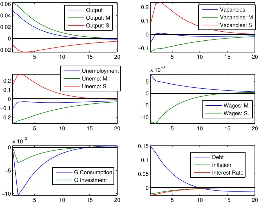
Sectoral Technology Shocks
We begin with a positive, mean-reverting technology shock in the manufacturing sector as shown in figure 3. This shock increases manufacturing sector output and reduces marginal costs in this sector. Lower marginal costs - via the New Keynesian Phillips curve - imply lower prices and inflation falls. The model generates a sectoral shift towards the manufacturing sector as a consequence of higher relative productivity in this sector. While manufacturing sector output increases, service sector output decreases. Nevertheless, the increase in manufacturing sector output overcompensates reduced output in the service sector and aggregate output increases. Our findings contrast the "average out" view of Lucas (1977) that sectoral reallocations should have only very limited effects on aggregate measures. This does not hold true in a sectoral model with labor market frictions and sticky prices. As shown in Wesselbaum (2011) sticky prices are crucial to obtain this result. They create an amplifying effect in the manufacturing sector and through the positive effects of lower interest rates set by the monetary authority.
5 10 15 20 −0.02
0 0.02 0.04 0.06
Output Output: M Output: S
5 10 15 20
−0.1 0 0.1
0.2 Vacancies
Vacancies: M Vacancies: S
5 10 15 20
−0.2 −0.1 0 0.1 0.2
Unemployment Unemp: M. Unemp: S.
5 10 15 20
−10 −5 0 5
x 10−3
Wages: M. Wages: S.
5 10 15 20
−10 −5 0
x 10−3
G Consumption G Investment
5 10 15 20
0 0.05 0.1 0.15
[image:15.595.190.450.110.321.2]Debt Inflation Interest Rate
Figure 3: Impulse responses to an estimated technology shock in the manufacturing sector.
service sector. The technology shock increases the value of a match and leads firms to increase the number of employees. Adjustments mainly occur along the exit side. Firms prefer to reduce the number of separations then to post more vacancies. The reason is that reduced separations are immediately effective and are costless, while vacancies are costly and only become effective in the next period. The opposite effects are obtained for the service sector labor market. To a large extend, this is driven by much larger vacancy posting costs in the manufacturing sector than in the service sector and the larger steady state separation rate in the manufacturing sector.
Higher output and lower inflation lead the monetary authority to lower the interest rate to stimulate private consumption. Fiscal policy responds countercyclically and, hence, government consumption and investment activities are reduced.
Turning to the service-sector technology shock we observe significant differences. We find that the output responses are much more persistent compared to the manufacturing sector shock. Al-though aggregate output does not increase as much as in the previous case, its persistence is much higher. This is partly explained by the small adverse spillover effects towards the manufacturing sector. Manufacturing sector output does decrease but not as much as service sector output did in the previous scenario. This does have effects on the labor markets. Because the increase of aggregate output is more persistent, unemployment decreases by more as the discounted, expected profits from an additional worker are larger. Further, this also explains the larger impact on real wages, as workers have a larger bargaining power in the service sector.
5 10 15 20 0
0.02 0.04
0.06 Output
Output: M Output: S
5 10 15 20
−0.4 −0.3 −0.2 −0.1 0
Vacancies Vacancies: M Vacancies: S
5 10 15 20
−0.6 −0.4 −0.2 0
Unemployment Unemp: M. Unemp: S.
5 10 15 20
0 0.01 0.02 0.03
Wages: M. Wages: S.
5 10 15 20
−3 −2 −1
0x 10
−3
G Consumption G Investment
5 10 15 20
0 0.05
0.1 Debt
[image:16.595.188.453.125.331.2]Inflation Interest Rate
Figure 4: Impulse responses to an estimated technology shock in the service sector.
We begin with a positive, mean-reverting shock to government consumption. Figure 5 presents the impulse response functions. First of all, we find that the effects, aggregate as well as sectoral, are fairly small. Higher government consumption does increase aggregate and sectoral output through the demand channel. Hump-shaped impulse responses show that the model generates a persistent adjustment path towards the steady state. We find symmetric effects in both labor markets. Higher demand creates an incentive for firms to increase employment and do so by reducing firing. The differences in vacancy posting costs and bargaining power across sectors leads to small differences in the reaction of the two sectors. We find that the service sector reacts more strongly to the consumption shock, which is mainly driven by the stronger reaction in real wages.
5 10 15 20 0
1 2 3
x 10−6
Output Output: M Output: S
5 10 15 20
−3 −2 −1 0
x 10−5
Vacancies Vacancies: M Vacancies: S
5 10 15 20
−3 −2 −1 0 1
x 10−5
Unemployment Unemp: M. Unemp: S.
5 10 15 20
0 10 20
x 10−7
Wages: M. Wages: S.
5 10 15 20
0 5 10 15
x 10−3
G Consumption G Investment
5 10 15 20
−0.02 −0.01 0
[image:17.595.192.426.79.314.2]Debt Inflation Interest Rate
Figure 5: Impulse responses to an estimated government consumption shock.
such that unemployment increase in the medium-run. Again, due to the different structural labor market parameters, the reaction in the service sector is larger compared to the manufacturing sector. Finally, we find that the fiscal rules imply a decrease in government consumption but, as the increase in investment is larger than the drop in consumption, debt increases.
We can conclude that government investment is far more effective in increasing aggregate and sectoral output levels than government consumption. However, this also comes at a cost: govern-ment investgovern-ment leads to increased unemploygovern-ment over the medium-run after an initial drop in the unemployment rate. Further, government debt increases sizably. Both observations are not present for government consumption shock.
4
Conclusion
The Great Recession has rescuscitated the interest in the effects of fiscal policy to counter adverse effects on output and labor markets. However, academic research related to the sectoral (labor market) effects of fiscal policy is rather sparse.
5 10 15 20 0
0.02 0.04 0.06 0.08
Output Output: M Output: S
5 10 15 20
−0.3 −0.2 −0.1 0
Vacancies Vacancies: M Vacancies: S
5 10 15 20
−0.4 −0.2 0
Unemployment Unemp: M. Unemp: S.
5 10 15 20
0 0.01 0.02 0.03
Wages: M. Wages: S.
5 10 15 20
−0.02 −0.01 0 0.01 0.02
G Consumption G Investment
5 10 15 20
0 0.5 1
[image:18.595.185.428.88.322.2]Debt Inflation Interest Rate
Figure 6: Impulse responses to an estimated government investment shock.
for discretionary interventions. Then, the model is estimated on U.S. time series using Bayesian methods.
We find several interesting results. Compared to the service sector, the manufacturing sector labor market has higher job flows in steady state and workers have a lower bargaining power. Further, vacancy posting costs are roughly five times lower. Government debt has no significant impact on fiscal spending. Government consumption and investment respond solely to movements in output, i.e. are automatic stabilizers. Government consumption reacts roughly three times as much to variations in output than government investment.
Business cycle fluctuations of sectoral and aggregate output as well as the inflation rate are mainly driven by government investment shock. This finding is likely to be biased due to the absence of private capital. Employment appears to be driven by the sectoral technology shocks and, for the manufacturing sector, the aggregate technology shock.
Both types of fiscal spending shocks lead to an increase in sectoral and aggregate output. For the labor market, unemployment decreases on impact but increase in the medium-run. Overall, we find that investment shocks create larger real effects than consumption shocks. However, they generate a large increase in government debt that only slowly converges back to the steady state.
References
[1] Aschauer, D. A., 1989. "Does Public Capital Crowd Out Private Capital?"Journal of Monetary Economics, 24 (September): 171-188.
[2] Bénétrix, A. and P. Lane, 2010. "Fiscal Shocks and The Sectoral Composition of Output,"
Open Economies Review, 21(3): 335-350.
[3] Bernstein, J. and C. Romer, 2009. "The Job Impact of the American Recovery and Reinvest-ment Plan". The White House.
[4] Bouakez, H., M. Guillard, and J. Roulleau-Pasdeloup, 2014. "Public Investment, Time to Build, and the Zero Lower Bound." CIRPÉE Working Paper 14-02.
[5] Bouakez, H., D. Larocque, and M. Normandin, 2013. "Separating the Wheat from the Chaff: A Disaggregate Analysis of the Effects of Public Spending in the U.S." Mimeo.
[6] Davis, S. J., 2001. "The quality distribution of jobs and the structure of wages in search equilibrium." NBER Working Paper, No. 8434.
[7] Davis, S. J. and J. C. Haltiwanger, 2001. "Sectoral job creation and destruction responses to oil price changes."Journal of Monetary Economics 48(3): 465-512.
[8] Davis, S. J., R. J. Faberman, and J. C. Haltiwanger, 2009. "The Establishment-Level Behavior of Vacancies and Hiring."Quarterly Journal of Economics, 128(2): 581-622.
[9] Di Pace, F. and S. Villa. 2013. "Redistributive effects and labour market dynamics." Center for Economic Studies - Discussion papers ces13.23.
[10] Evans, P., and G. Karras, 1994. "Are Government Activities Productive? Evidence from a Panel of U.S. States,"Review of Economic and Statistics, 76 (1): 1-11.
[11] den Haan, W. J., G. Ramey, and J. Watson, 2000. "Job destruction and the propagation of shocks."American Economic Review 90(3): 482-498.
[12] Kydland, F. E. and E. C. Prescott, 1982. "Time to build and aggregate fluctuations." Econo-metrica, 50(6): 1345-1370.
[13] Krause, M. U. and T. A. Lubik, 2007. "The (ir)relevance of real wage rigidity in the New Keynesian model with search frictions."Journal of Monetary Economics 54(3): 706-727.
[14] Lamo, A., J., Messina, and E. Wasmer, 2006. "Are specific skills an obstacle to labor market adjustment? Theory and an application to the EU enlargement." European Central Bank Working Paper, No. 585.
[16] Lubik, T. A., forthcoming. "Aggregate Labour Market Dynamics in Hong Kong." Pacific Economic Review.
[17] Lubik, T. A., 2009. "Estimating a Search and Matching Model of the Aggregate Labor Market."
Economic Quarterly, 95: 101-120.
[18] Lucas, R. E., 1977. "Understanding business cycles." In: Brunner, K., Meltzer, A. (Eds.),
Carnegie Rochester Series on Public Policy, 5: 7-29.
[19] Merz, M., 1995. "Search in the labor market and the real business cycle."Journal of Monetary Economics 36 (2): 269-300.
[20] Monacelli, T. and R. Perotti, 2008. "Openness and the Sectoral Effects of Fiscal Policy," Journal of the European Economic Association, MIT Press, vol. 6(2-3), pages 395-403
[21] Mortensen, D. and C. A. Pissarides, 1994. "Job creation and job destruction in the theory of unemployment."Review of Economic Studies 61(3): 397-415.
[22] Obstbaum, M., 2011. "The Role of Labour Markets in Fiscal Policy Transmission." Bank of Finland Discussion Papers 16/2011.
[23] Rotemberg, J., 1982. "Monopolistic price adjustment and aggregate output." Review of Eco-nomic Studies 49(4): 517-531.
[24] Tapp, S., 2007. "The dynamics of sectoral labor adjustment." Queen’s Economics Department Working Paper, No. 1141.
[25] Wesselbaum, D., forthcoming. "Labor Market Dynamics in Australia." Australian Economic Review.
[26] Wesselbaum, D., 2011. "Sector-specific productivity shocks in a matching model," Economic Modelling, 28(6): 2674-2682.
0.05 0.1 0.15 0 50 100 150 200 ρ
0.05 0.1 0.15 0
50 100
ρ
0.4 0.5 0.6 0
20 40
η
0.4 0.5 0.6 0 20 40 60 80 η
0.020.040.060.08 0.1 0.12 0 50 100 150 200 c
0.4 0.5 0.6 0
20 40
µ
0.4 0.5 0.6 0 20 40 60 80 µ
0.02 0.04 0.06 0
50 100 150
δ
0 0.2 0.4 0.6 0 20 40 60 80 γ
0 0.2 0.4 0.6 0
200 400 600
γ
0.2 0.4 0.6 0
20 40
λ
0 0.2 0.4 0.6 0
20 40
λ
Service
Manufacturing Manufacturing Service
Service Manufacturing
Manufacturing
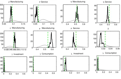
[image:21.595.93.500.85.350.2]Investment Consumption Investment Consumption
Figure 7: Prior vs. Posterior.
−0.10 0 0.1 0.2
50 100
α
−0.10 0 0.1 0.2
50 100
α
1.4 1.5 1.6
0 20 40 60
φ π
0 0.1 0.2
0 20 40 60
φ
30 40 50
0 0.5 1
ψ
0.2 0.4 0.6 0.8
[image:21.595.91.503.91.643.2]0 10 20 30 α y Manufacturing Service