Method of Dynamic VaR and CVaR Risk Measures Forecasting for Long Range Dependent Time Series on the Base of the Heteroscedastic Model

(1)

http://www.scirp.org/journal/ica ISSN Online: 2153-0661

ISSN Print: 2153-0653

Method of Dynamic VaR and CVaR Risk

Measures Forecasting for Long Range

Dependent Time Series on the Base of the

Heteroscedastic Model

Nataliya D. Pankratova, Nataliia G. Zrazhevska

Institute for Applied Systems Analysis, National Technical University of Ukraine “Kyiv Polytechnic Institute”, Kyiv, Ukraine

Abstract

The paper proposes a new method of dynamic VaR and CVaR risk measures forecasting. The method is designed for obtaining the forecast estimates of risk measures for volatile time series with long range dependence. The me-thod is based on the heteroskedastic time series model. The FIGARCH model is used for volatility modeling and forecasting. The model is reduced to the AR model of infinite order. The reduced system of Yule-Walker equations is solved to find the autoregression coefficients. The regression equation for the autocorrelation function based on the definition of a long-range dependence is used to get the autocorrelation estimates. An optimization procedure is proposed to specify the estimates of autocorrelation coefficients. The proce-dure for obtaining of the forecast values of dynamic risk measures VaR and CVaR is formalized as a multi-step algorithm. The algorithm includes the fol-lowing steps: autoregression forecasting, innovation highlighting, obtaining of the assessments for static risk measures for residuals of the model, forming of the final forecast using the proposed formulas, quality analysis of the results. The proposed method is applied to the time series of the index of the Tokyo stock exchange. The quality analysis using various tests is conducted and con-firmed the high quality of the obtained estimates.

Keywords

Dynamic VaR, CVaR, Forecasting, Long Range Dependence, Hurst Parameter, Heteroscedastic Model

1. Introduction

VaR (Value-at-Risk) and CVaR (Conditional Value-at-Risk) have become the How to cite this paper: Pankratova, N.D.

and Zrazhevska, N.G. (2017) Method of Dynamic VaR and CVaR Risk Measures Forecasting for Long Range Dependent Time Series on the Base of the Heteroscedas-tic Model. Intelligent Control and Automa-tion, 8, 126-138.

https://doi.org/10.4236/ica.2017.82010

Received: March 30, 2017 Accepted: May 23, 2017 Published: May 26, 2017

http://creativecommons.org/licenses/by/4.0/

(2)

standard measures of market risk management. Their popularity has led to a large number of publications on this topic in recent years. Definition, descrip-tion of the properties and comparative analysis of these risk measures can be found, for example, in [1] [2] [3]. Various methods for their evaluation and fo-recasting that represents different approaches are proposed. Most of the me-thods that provide explicit formulas for CVaR estimation are described in [4]. Optimization approach for CVaR evaluation is given in [5] [6]. Non-parametric methods of estimation can be found, for example, in [7] [8]. A large number of works devoted to the method of VaR and CVaR estimating based on the sto-chastic time series model. The basic ideas of the approach can be found for ex-ample in [2] [9] [10]. A significant number of works show the practical applica-tion of the approach for estimating and forecasting of stock indices, see for ex-ample [10] [11] [12] [13].

At the same time, during the global financial turmoil, the problem of con-structing of new approaches for VaR and CVaR estimating and forecasting re-mains relevant. In this paper, we propose a new method for VaR and CVaR pre-diction for financial time series. The method takes into account the most statis-tically significant extreme values of data and the presence of the long-range de-pendence that is typical for financial time series [2] [14]. For the convenience of practical application, the method is formulated as an incremental algorithm. At each step, the system of tests is proposed to evaluate the quality of the obtained results.

The proposed algorithm is used for forecasting VaR and CVaR for the time series of daily log return Nikkey225 Stock Index. The analysis of the obtained forecast estimates confirms their high quality. The formatter will need to create these components, incorporating the applicable criteria that follow.

2. Key Definitions

The continuously distributed random variable

{

X tt, ∈Z

}

with finite mean

de-fined on the probability space

(

Ω Ψ Ρ, _t, _t

)

is considered. Here Ψ_t is the

in-formation set containing all available at the time t information about the time series. Series

{

2

}

, t

X t∈Z is assumed to be stationary. It is accepted that the time series has the property of the long-range dependence [15]: there is

0< <

γ

1 and cr >0 so that:

( )

(

)

( )

(

)

{ }

lim r 1, Corr t, t k , 0

k k c k k X X k N

γ

ρ

−

ρ

+

→∞ = = ∈ ∪ (1)

For a fixed confidence level α dynamic risk measures VaR and CVaR

are defined as [9]:

(

)

{

[

]

}

VaRαt t+h =inf x∈ ΡR t Xt h+ ≤x ≥

α

,

(

)

(

)

CVaR VaR ,

t

t t

t h t h

t h E X X t h

α + = Ψ  + + ≥ α + 

[ ]

t

E_Ψ ⋅ denotes expectation with respect to Ψ_t.

(3)

(

)

CVaRt_α t+h where t is an arbitrary moment of time. The forecasting val-ues are determined by extrapolation of the valval-ues of this model (21 cm × 28.5 cm).

3. Forecast Methodology

In the article [16], the most popular methods for dynamic VaR and CVaR

estimating are analyzed, their classification is given and the recommendations for their use are proposed. In accordance with the formulated in the article the structural scheme of selection of dynamic risk measures estimation the approach based on a stochastic time series model is chosen.

Suppose that the time series

{

X tt, ∈Z

}

is a trajectory of stochastic process,

that is:

t t t t t t

X =µ ε+ =µ σ+ Z (2) where conditional mean µt and variation σt are defined on the information space Ψt,

{ }

~

( )

0,1

iid

t t

Z F (independent, identically distributed random va-riables with a conditional distribution function Ft

( )

0,1 ). Let Z is a random

variable with the same distribution as any random variable from

{ }

Zt . Then [2] [9] [10]:

( )

1 ,

,

VaR VaR ,

CVaR CVaR .

t

k t k t k t k t k

t

k t k t k

F Z

Z

α α

µ α σ µ σ

µ σ

−

+ + + +

+ +

= + = +

= + (3)

It is necessary to construct the forecast model for σt to determine its P days forecast and to estimate VaR and CVaR for a random variable Z. Then the forecasting values for dynamic risk measures can be found under the following formulas:

( )

VaR VaR ,

CVaR CVaR ..

t P

t P t P

t p

t P t P

Z Z α α α α µ σ µ σ + + + + + + = +

= + (4)

Hereinafter it is assumed that the trend, that defines µt, is absent (or re-moved from the data) [2]. Please do not revise any of the current designations.

4. An Algorithm for Constructing the Dynamic Risk

Measures VaR and CVaR Forecast Taking into

Account the Long-Range Dependence Presence

For the convenience of the practical application the proposed method for VaR

and CVaR forecasting is formulated as an incremental algorithm.

Step 1. For the time series a time series of variances (TSV) is constructed. General analysis of the studied time series and the TSV is carried out, the de-pendence of time series members (and their squares) from their previous values; the volatility and normality are analyzed.

Step 2. The TSV is tested on the long-range dependence. The Hurst parame-ter is estimated using five standard methods: the aggregated variance method, the method of absolute values of the aggregated series, the periodogram method, the method of residuals of regression, the R/S method [17]. Average value Hmn

(4)

is chosen as the Hurst parameter estimation.

Step 3. The model for σt forecasting is estimated using the FIGARCH model and taking into account the long-range dependence of the WFD. The ac-tualization of the model by reducing it to the model AR (∞) is performed. The method of smoothing of the autocorrelation function (ACF) proposed by the authors in [18] (the new method) is used. The least square method is used to de-termine the autoregression coefficients

(

a1,,aN,

)

′. So the problem is re-duced to the infinite system of Yule-Walker equations [18]:

1 0

, 0, , .

j i i j j a i ρ ρ ∞ + − = = = ∞

∑

 (5)

The regression equation for ACF based on the definition of the long-range dependence (1) is used to get estimates for

( )

(

)

2 2

1 2

: 2 1 H

i k H H k k

ρ ρ

₌

α

₋ − ₊

α

₊

ε

, ε −k iid, k0≤ ≤k N. With the help of the optimization procedure [17] the Hurst parameter estimate and the esti-mates

ρ



( )

k are corrected.

Using

ρ



( )

k instead of ρk the reduced system of normal Equations (5) is constructed and using the Holetskogo method the vector of assessments

(

1

)

ˆ _ˆ_, _,_ˆ

N N

a = a  a ′ is found. As it is shown in [19] the solution of the reduced system converges to the exact solution.

The lag of the reduced AR model M≤N is determined using the informa-tion criterions: AIK (Akaike informainforma-tion criterion), HQC (Hannan-Quinn in-formation criterion), SBIC (Bayesian inin-formation criterion) [14]. The lag value is chosen on the basis of minimum deviation.

The quality of the obtained AR model is checked. The variance ratio test [20]

is used to test if the residuals of the model are iid (independent and identically distributed). The resulting model is used to obtain σˆ_t.

Step 4. The residuals of the model (2) are analyzed. Using σˆ_t (step 3) the

implementations of a random variable _: ˆ _ˆ

t t t t

Z Z =X

σ

are built. Zt are ana-lyzed on iid (the variance ratio test) and other properties. In accordance with the results using the classification scheme given in [21], the method to get

( )

VaR_α Z and CVaR_α

( )

Z estimates is chosen. The estimates VaRα

( )

Z ,



_{( )}

CVaRα Z are obtained.

Step 5. With the results of steps 3 and 4 the model for dynamic risk measures estimating (3) is ready. After building the dynamic risk measures estimations



VaRt_α и CVaRt_α their quality is analyzed using the Kupiec test, the

Kristof-fersen test and the V test [10] [16].

Step 6. The built dynamic risk measures model is used to get the forecast. Using the model from step 3 the P-step forecast for σt is built by the formu-las:

2 2

1

ˆ ˆ ˆ , 1, , 1, , .

M p

l p i l i

i p

a l N p P

σ₊ + σ_{− +}

=

∑

= +  =  (6)

Using the estimates VaRα

( )

Z , CVaRα

( )

Z (step 4) the P-step forecast for dynamic risk measures VaRt Pα

+

and CVaRαt P +

(5)

index of the time series is increased by P and the procedure is repeated as many times as necessary. Thus in each cycle of the algorithm application the model is updated to take into account new data.

Step 7. Using the back testing procedure, the quality of the predicted values 

VaRαt P +

and CVaRt Pα +

(step 6) is checked, the prediction errors ME, MAE, MSE are calculated. For CVaR estimates the BPoE-test [22] is used.

Schematic description of the proposed method is shown in Figure 1. Please take note of the following items when proofreading spelling and grammar.

5. Numerical Testing of the Algorithm

To demonstrate the proposed algorithm a forecast for dynamic risk measures

(

α

=0.9

)

for the time series of log returns on a daily basis is built. Data are col-lected from the oldest and the most well-known index of Asian markets

Nikkey 225 Stock Index (the time series N225 _RED)—a composite index of the 225 largest companies publicly traded in Tokyo Stock Exchange for the

pe-riod from 2005 to 2015. N225 _RED has a relatively low homogeneous vola-tility. The aim of this study is to forecast risk measures at a regular market beha-vior, so data without three time intervals with high volatility of the global finan-cial system (01.07.2008-01.07.2009, 01.01.2011-01.07.2011, 01.02.2013-01.12.2013) are considered. Historical data of Nikkey 225 Stock Index are not available

[image:5.595.259.488.432.616.2]

on-line, but upon request.

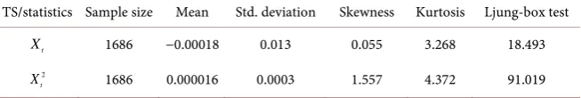
Table 1 demonstrates the descriptive statistics for the time-series

( )

Xt and the squared series

( )

2

t X .

[image:5.595.212.539.681.736.2]

Figure 1. Schematic description of the proposed method of dynamic risk measures VaR and CVaR forecasting.

Table 1. Basic descriptive statistics of the N225_RED.

TS/statistics Sample size Mean Std. deviation Skewness Kurtosis Ljung-box test

t

X 1686 −0.00018 0.013 0.055 3.268 18.493

2

t

X 1686 0.000016 0.0003 1.557 4.372 91.019

Volatility modeling using FIGARCH

Obtaining static VaR, CVaR _{Volatility forecasting}

Dynamic VaR, CVaR forecasting residuals of the model

data data

Preliminary data analysis

(6)

Skewness is about 0 and kurtosis is about 3, so the distributions are close to normal. Ljung-Box test [2] results for m=7 confirm the dependence of data

(and squared data) on their previous values (the values of Q-statistic are larger than critical value 12.017).

Consider the half of the general sample-843 values. The estimates of the Hurst parameter are Hmn=0.7387



and Hopt =0.7281 

(step 2). These values con-firm the long-range dependence of the time series.

Simulate σt (step 3) using the method SACF (the designation _ SACF) and for comparison the standard methodology (the designation _st). The standard methodology uses the AR M

( )

model with the coefficients found by the maximum likelihood method (MLH). The lag of the reduced AR model is

55

M = . The results of the variance ratio test (0.99 < 1.96 for the SACF

me-thod and 0.69 < 1.96 for the standard meme-thod) confirm that the residuals of the models are iid.

For both models Zt are found (step 4) and their analysis is carried out. The results of the variance ratio test (0.98 < 1.96 for the method SACF and 0.97 <

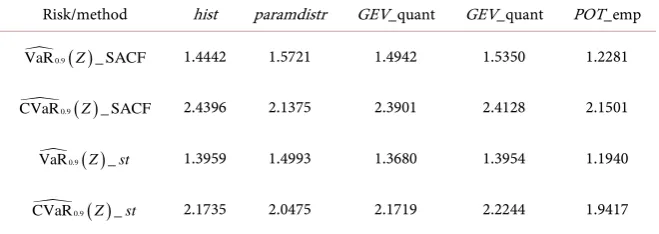
1.96 for the standard method) show that the residuals of the model (2) are iid. Estimates VaR0.9

( )

Z , CVaR0.9

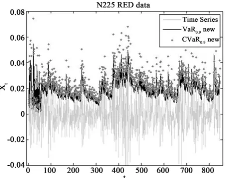
. Table 2 demonstrates the results of the estimating.

Using the results of steps 3, 4 estimates (3) of the dynamic VaR0.9 t

and CVaR0.9 t

(step 5) are obtained. Figure 2 demonstrates the simulated dynamic VaR0.9_ SACF t

and CVaR0.9_ SACF t

(first 836 values) where the explicit formulas under the assumption of a normal distribution

(

paramdistr

)

were used for risk measures

[image:6.595.261.488.520.700.2]

model residuals estimating.

(7)

[image:7.595.210.540.97.214.2]

Table 2. The estimates of the statics VaR0.9

( )

Z , CVaR0.9

( )

Z .

Risk/method hist paramdistr GEV_quant GEV_quant POT_emp

0.9_{( )}

VaR Z _ SACF 1.4442 1.5721 1.4942 1.5350 1.2281

0.9_{( )}

CVaR Z _ SACF 2.4396 2.1375 2.3901 2.4128 2.1501

0.9_{( )}

VaR Z _st 1.3959 1.4993 1.3680 1.3954 1.1940

0.9_{( )}

CVaR Z _st 2.1735 2.0475 2.1719 2.2244 1.9417

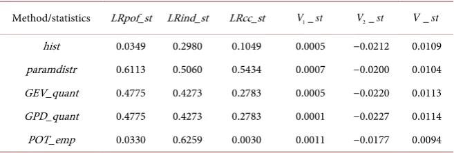
Conduct the analysis of quality (step 5) for VaR0.9 t

estimates using the Ku-piec test (p−values of statistics LRpof), the Kristoffersen test (p− values of statistics LRind) and their combination (p− values of statistics LRcc). The

obtained estimates are reliable if p− values exceed the given significance level (0.1 in our case). To analyze the CVaR0.9

t

estimates the V test with statistics

1

V, V2, V is used. If the estimates are good the statistics, V1, V2, V are close to zero. Table 3 presents the results of the analysis of the dynamic risk measures estimates for the SACF method and Table 4 for the standard

me-thod.

The analysis of the results shows that the method paramdistr (on the

as-sumption of the normal distribution of residuals) gives the best VaR0.9 t

esti-mates for both methods: p− values of statistics are essentially more than 0.1. This is consistent with the results of the basic analysis (Table 1) and is con-firmed by the results of the Jarque-Bera test [2] conducted for Zt (5.624 < 5.649 and 4.38 < 5.649 for both proposed and standard methods, respectively). At the same time, all estimates obtained with POT_ emp method show the

poor quality. The popular historical simulated method

(

hist

)

gives quality

es-timates only with the SACF method. In addition all values of statistics for the SACF method are greater than the appropriate values for the standard method.

V-test shows good results for both SACF and standard methods.

The built models are used for dynamic risk measures forecasting. Forecasting procedure is performed on the window length equal to the half of the general sample power (843 values). 5-day

(

P=5

)

forecast is built (see Figure 2). Thus,

it is assumed that the parameters of the model are adequate for a period 5 (or more) days, the estimates of static risk measures at the forecast horizon are un-changed.

The forecasting procedure (steps 2 - 6) is repeated 168 times, and each time 5 new values (the accumulation window) are added. Table 5 presents minimum

min

H , maximum Hmax and average Hmn values of the Hurst parameter ob-tained for the windows.

Table 5 shows, the values of the Hurst parameter confirm the long-range

(8)

[image:8.595.208.540.113.212.2]

Table 3. The results of the analysis of the dynamic risk measures estimates (SACF method).

Method/statistics LRpof_SACF LRind_SACF LRcc_SACF V1_ SACF V2_ SACF V_ SACF

[image:8.595.210.539.255.366.2]

hist 0.1289 0.5949 0.6058 −0.0002 −0.0233 0.0118 paramdistr 0.7968 0.6467 0.7536 0.0019 −0.0189 0.0110 GEV_quant 0.3477 0.3359 0.6088 0.0012 −0.0228 0.0120 GPD_quant 0.1986 0.4498 0.6688 0.0013 −0.0230 0.0122 POT_emp 0.0253 0.2610 0.0206 0.0011 −0.0249 0.0130

Table 4. The results of the analysis of the dynamic risk measures estimations (standard method).

Method/statistics LRpof_st LRind_st LRcc_st V1_st V2_st V_st

[image:8.595.211.539.400.496.2]

hist 0.0349 0.2980 0.1049 0.0005 −0.0212 0.0109 paramdistr 0.6113 0.5060 0.5434 0.0007 −0.0200 0.0104 GEV_quant 0.4775 0.4273 0.2783 0.0005 −0.0220 0.0113 GPD_quant 0.4775 0.4273 0.2783 0.0001 −0.0227 0.0114 POT_emp 0.0330 0.6259 0.0030 0.0011 −0.0177 0.0094

Table 5. Hurst parameter estimates.

H/method abs. values Aggregated _variance Residuals of _{regression Periodogram} R/S Optimization

min

H 0.7262 0.6872 0.6241 0.6777 0.7044 0.7199

max

H 0.7837 0.7872 0.7246 0.8854 0.7680 0.7438

mn

H 0.7546 0.7445 0.6758 0.7926 0.7356 0.7276

Figure 3 demonstrates the results of variance forecasting using (6) with SACF and standard methods.

Visual comparison of the predicted and real values shows that the proposed new method better describes the dynamic behavior of the time series. Extreme values obtained with the new method are much closer to real values. The new method also exhibits less lag in extreme values determination. This can be ex-plained by the fact that the new method uses the ACF prediction and takes into account the property of the long-range dependence. It should also be noted that the optimization procedure in the determination of the Hurst parameter has sig-nificantly improved the forecast stability.

Minimum, maximum and average values of the static risk measures for dif-ferent windows are shown in Table 6 (the SACF method) and Table 7 (the

standard method).

(9)

[image:9.595.242.508.69.280.2]

Figure 3. Real values of variance for real data and forecast estimates obtained by SACF

[image:9.595.209.540.355.526.2]

and standard methods.

Table 6. VaR0.9

( )

Z , CVaR0.9

( )

Z estimates for different windows (SACF method).

Method hist paramdistr GEV_quant GEV_quant POT_emp

0.9_{( )}

VaR Z _ SACF min 1.4121 1.5115 1.4465 1.4811 1.2280

0.9_{( )}

VaR Z _ SACF max 1.4645 1.5849 1.5325 1.5490 1.7623

0.9_{( )}

VaR Z _ SACFmn 1.4379 1.5414 1.4898 1.5135 1.5103

0.9_{( )}

CVaR Z _ SACF min 2.2466 1.5414 2.2278 2.2607 2.1501

0.9_{( )}

CVaR Z _ SACF max 2.4645 2.1536 2.4217 2.4364 2.6978

0.9_{( )}

CVaR Z _ SACFmn 2.3254 2.1038 2.3013 2.3298 2.4001

Table 7. VaR0.9

( )

Z , CVaR0.9

( )

Z estimates for different windows(standardmethod).

Method hist paramdistr GEV_quant GEV_quant POT_emp

0.9_{( )}

VaR Z _stmin 1.2462 1.2927 1.2541 1.2717 1.1921

0.9_{( )}

VaR Z _stmax 1.4305 2.3181 1.4411 1.4011 1.5898

0.9_{( )}

VaR Z _stmn 1.3125 1.4398 1.3241 1.3372 1.3706

0.9_{( )}

CVaR Z _stmin 1.9061 1.7723 1.9038 1.9390 1.8842

0.9_{( )}

CVaR Z _stmax 2.3166 3.1949 2.3825 2.4033 2.4764

0.9_{( )}

[image:9.595.210.540.564.741.2]

(10)

ues (max-min) for the SACF method is less than the range of values for the

standard method due to the fact that the proposed method explicitly uses the smoothing procedure of ACF and as a result the distribution function is more stable.

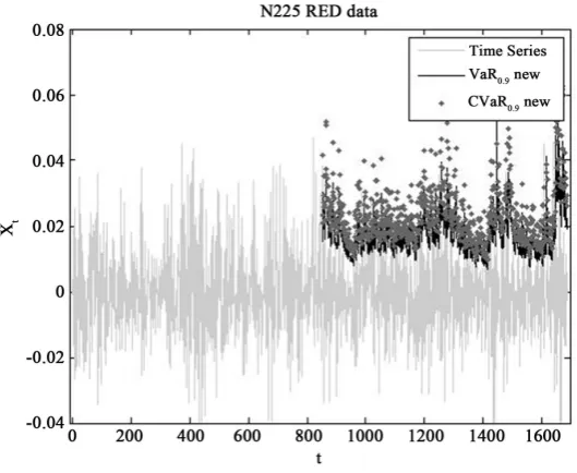
The obtained results are used to get the time series of dynamic risk measures estimates (3). As an example Figure 4 shows the forecast estimates for VaR0.9

t

andCVaR0.9 t

, obtained with the use of the paramdistr method. The prediction errors of VaR0.9

t

and CVaR0.9 t

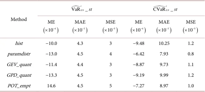
for both methods (for dif-ferent methods of static risk measures estimating) are shown in Table 8 and Ta-ble 9.

Table 8 and Table 9 show that the prediction errors obtained for the SACF

method is less than the prediction errors obtained for the standard method. This proves the advantage of the proposed method. In addition Table 8 shows that methods hist and paramdistr gives the best estimates. This once again

con-firms the previously accepted hypothesis of data normal distribution. The quality of built CVaR0.9

t

[image:10.595.242.507.339.556.2]

forecast estimates is analyzed with BPoE test.

Table 10 shows the BPoE values obtained for the initial data

( )

real and for the

Figure 4. Forecast estimates for VaR0.9 t

and CVaR0.9 t

[image:10.595.212.539.612.736.2]

for 168 windows.

Table 8. The prediction errors of VaR0.9 t

and CVaR0.9 t

(SACF method).

Method

0.9

VaR _ SACF

t _

0.9

10−

×

(11)

[image:11.595.210.539.92.239.2]

Table 9. The prediction errors of VaR0.9 t

and CVaR0.9 t

(standard method).

Method

0.9

VaR _

t

st CVaR0.9_

10−

×

[image:11.595.210.541.275.342.2]

hist −10.0 4.3 3 −9.48 10.25 1.2 paramdistr −13.0 4.5 4 −6.42 7.93 0.8 GEV_quant −11.4 4.4 3 −8.87 9.73 1.1 GPD_quant −13.3 4.5 3 −9.19 9.99 1.2 POT_empt 14.6 4.5 5 −7.27 8.97 1.0

Table 10. Results of BPoЕ-test for CVaR0.9 t

.

Method hist paramdistr GEV_quant GEV_quant POT_emp SACF meth 0.9018 0.9062 0.9102 0.9114 0.9102

st meth 0.8838 0.9154 0.8838 0.8886 0.8958 real 0.9102 0.9034 0.9162 0.9198 0.8898

forecast estimates with the use of the new method

(

SACF meth

)

and the

stan-dard method

(

st meth

)

. These values are compared with the chosen level of

risk measures

α

=0.9. The results show the high quality of the forecast

esti-mates CVaR0.9 t

obtained by the new method.

Table 10 may be used to liken the methods used for forecasting by comparing the value of confidence level α_{for predicted and real risk measures values. The}

standard method based on paramdistr demonstrates the best results. At the

same time, the proposed method shows the best results with the historical simu-lation method

( )

hist . Table 10 shows that the deviation of α for the new

method

(

0.84%

)

is substantially less than the deviation for the standard

me-thod

(

1.8%

)

.

6. Conclusion

In the article, a multi-step procedure for constructing the dynamic risk measures VaR and CVaR forecast is proposed. The procedure is designed for volatile series with the long-range dependence and is based on the heteroscedastic time series model. The optimization procedure for constructing and forecasting of ACF is used to find the model parameters. For the convenience of practical application, the prediction procedure is formulated as an algorithm. To test the proposed al-gorithm, the risk measures forecast for the time series of daily log return

Nikkey 225 Stock Index is built. Different tests carried out at different stages of

the algorithm confirm the good quality of the obtained estimates.

References

(12)

Risk. Mathematical Finance, 9, 203-228.https://doi.org/10.1111/1467-9965.00068

[2] Tsay, R.S. (2010) Analysis of Financial Time Series. 3rd Edition, John Wiley & Sons, Hoboken.https://doi.org/10.1002/9780470644560

[3] Yamai, Y. and Yoshiba, T. (2002) Comparative Analysis of Expected Shortfall and Value-at-Risk: Their Estimation Error, Decomposition and Optimization. Monetary and Economic Studies, 20, 57-86.

[4] Nadarajah, S., Zhang, B. and Chan, S. (2014) Estimation Methods for Expected Shortfall. Quantitative Finance, 14, 271-291.

https://doi.org/10.1080/14697688.2013.816767

[5] Rockafellar, R.T. and Uryasev, S.P. (2000) Optimization of Conditional Value-at- Risk. Journal of Risk, 2, 21-42.https://doi.org/10.21314/JOR.2000.038

[6] Rockafellar, R.T. and Uryasev, S.P. (2002) Conditional Value-at-Risk for General Loss Distributions. Journal of Banking & Finance, 26, 1443-1471.

[7] Scaillet, O. (2004) Nonparametric Estimation and Sensitivity Analysis of Expected Shortfall. Mathematical,14, 115-129.

https://doi.org/10.1111/j.0960-1627.2004.00184.x

[8] Chen, S.X. (2008) Nonparametric Estimation of Expected Shortfall. Journal of Fi-nancial Econometrics, 6, 87-107. https://doi.org/10.1093/jjfinec/nbm019

[9] Embrechts, P., Kaufmann, R. and Patie, P. (2005) Strategic Long-Term Financial Risks: Single Risk Factors. Computational Optimization and Applications, 32, 61-

90.https://doi.org/10.1007/s10589-005-2054-7

[10] Kjellson, B. (2013) Forecasting Expected Shortfall. An Extreme Value Approach. Bachelor’s Thesis in Mathematical Sciences, K7, 43.

[11] Koksal, B. and Orhan, M. (2013) Market Risk of Developed and Emerging Coun-tries during the Global Financial Crisis. Emerging Markets. Finance & Trade, 49, 20-34.https://doi.org/10.2753/REE1540-496X490302

[12] Lee, T.-H., Bao, Y. and Saltoglu, B. (2006) Evaluating Predictive Performance of Va- lue-at-Risk Models in Emerging Markets: A Reality Check. Journal of Forecasting, 25, 101-128.https://doi.org/10.1002/for.977

[13] Yoon, S.-M. and Kang, S.-H. (2013) VaR Analysis for the Shanghai Stock Market.

The Macrotheme Review, 2, 89-95.

[14] Zivot, E. and Wang, J. (2003) Modeling Financial Time Series with S-PLUS. Sprin-ger-Verlag, New York.https://doi.org/10.1007/978-0-387-21763-5

[15] Palma, W. (2007) Long-Memory Time Series: Theory and Methods. John Wiley & Sons, Hoboken.https://doi.org/10.1002/9780470131466

[16] Zrazhevska, N. (2016) Construction and Application of the Classification Scheme of Dynamic Risk Measures Estimating. Eureka: Physics and Engineering, 5, 67-80. https://doi.org/10.21303/2461-4262.2016.00162

[17] Pankratova, N.D. and Zrazhevska, N.G. (2015) Model of the Autocorrelation Func-tion of the Time Series with Strong Dependence. Problemi Upravleniya Informatik, 5, 102-112.

[18] Zrazhevska, N.G. (2015) Smoothed Autocorrelation Function Method for Predict-ing of Variation of Heteroscedastictime. Systemnidoslidzhennya ta informacijni-texnologiyi, 2, 97-108.

[19] Zrazhevskij, A.G. (2011) System Approach to Restoring Functional Dependencies of Non-Stationary Time Series with Different Structures. Abstract of Dissertation for Scientific Degree of PhD, 20. (In Ukrainian)

(13)

Economy, 96, 893-920.https://doi.org/10.21303/2461-4262.2016.00162

[21] Zrazhevskaja, N.G. and Zrazhevskij, A.G. (2016) Classification of Methods for Risk Measures VaR and CVaR Calculation and Estimation. Systemnidoslidzhennya ta informacijnitexnologiyi, 3.

[22] Shang, D., Kuzmenko, V. and Uryasev, S. (2015) Cash Flow Matching with Risks Controlled by bPOE and CVaR. Research Report 2015-3, ISE Dept., University of Florida.

Submit or recommend next manuscript to SCIRP and we will provide best service for you:

Accepting pre-submission inquiries through Email, Facebook, LinkedIn, Twitter, etc. A wide selection of journals (inclusive of 9 subjects, more than 200 journals)

Providing 24-hour high-quality service User-friendly online submission system Fair and swift peer-review system

Efficient typesetting and proofreading procedure

Display of the result of downloads and visits, as well as the number of cited articles Maximum dissemination of your research work

Submit your manuscript at: http://papersubmission.scirp.org/