Estimation of Attributable Risk from Clustered Binary Data: The Case of Cross Sectional and Cohort Studies

http://www.scirp.org/journal/ojs ISSN Online: 2161-7198

ISSN Print: 2161-718X

Estimation of Attributable Risk from Clustered

Binary Data: The Case of Cross-Sectional and

Cohort Studies

Mohamed Shoukri

1*

, Allan Donner

2,3

, Futwan Al-Mohanna

1

1_{Department of Cell Biology, Research Center King Faisal Specialist Hospital & Research Center, Riyadh, KSA}

2_{Department of Epidemiology and Biostatistics, Schulich School of Medicine and Dentistry, University of Western Ontario,} London, Ontario, Canada

3_{Robarts Clinical Trials, Robarts Research Institute, London, Ontario, Canada}

Abstract

Effect sizes are estimated from several study designs when the subjects are in-dividually sampled. When the samples are the aggregate cluster of individuals, the within cluster correlation must be accounted for to construct correct con-fidence intervals, and to conduct valid statistical inference. The purpose of this article is to propose and evaluate statistical procedures for the estimation of the variance of the estimated attributable risk in parallel groups of clusters, and in a design dividing each of k clusters into two segments creating multiple sub-clusters. The estimated variance is the first order approximation and is obtained by the delta method. We apply the methodology and propose a Wald type confidence interval on the difference between two correlated attributable risks. We also construct a test on the hypothesis of equality of two correlated attributable risks. We evaluate the power of the proposed test via Monte-Carlo simulations.

Keywords

Correlated Binary Responses, Effect Size, Split-Cluster Design, Correlated Attributable Risks, Confidence Intervals, Monte-Carlo Simulations

1. Introduction

In the epidemiological research, it is important that the collected data are trans-lated into interpretable results which can be easily communicated to clinicians. The need for “translatable” evidence from research studies is of prime

impor-How to cite this paper: Shoukri, M., Donner, A. and Al-Mohanna, F. (2017) Estimation of Attributable Risk from Clus-tered Binary Data: The Case of Cross-Sec- tional and Cohort Studies. Open Journal of Statistics, 7, 240-253.

https://doi.org/10.4236/ojs.2017.72019

Received: March 2, 2017 Accepted: April 21, 2017 Published: April 24, 2017

Copyright © 2017 by authors and Scientific Research Publishing Inc. This work is licensed under the Creative Commons Attribution International License (CC BY 4.0).

tance in the evaluation of clinical interventions, because they hold the potential to immediately influence the course of patient treatment. When evaluating these studies, the examination of “Effect Size” or (ES) can be a useful measure of the comparative efficacy of the treatment under investigation. In randomized clini-cal trials, an effect size estimate quantifies the direction and magnitude of an ef-fect of an intervention.

When exposure and disease risk are measured on a binary scale, several meas-ures of effect size are in current use [1]. The odds ratio (OR), the relative risk (RR), and the population attributable risk (AR) are the most commonly used measures of effect size in clinical as well as analytic epidemiology.

The concept of AR was introduced in [2] and is a widely used measure of the amount of disease that can be attributed to a specific risk factor. The AR com-bines the relative risk (RR) and the prevalence of exposure P E

( )

to measure the public health burden of a risk factor by estimating the proportion of cases of a disease that would not have occurred if we remove the risk factor.

The concept of AR and its statistical characteristics have been reviewed in [3] and in several publications [4][5]. Statistical inferences on AR require the avail-ability of data from subjects randomly assigned to intervention groups. However, when the sampling strategy involves aggregate or clusters of individuals, adjust-ing for the effect of intracluster correlation is essential in order to conduct valid statistical inferences [6] and the references therein. However, the statistical pro- perties of estimators of AR when clusters are sampled have not yet been fully ex-plored. The fundamental objective of our work is to fill the gap of performing statistical inference on AR under the clustered binary data situation.

In this paper, we obtain the variance of the estimated AR under cluster sam-pling, focusing on cohort and cross-sectional designs. In Section 2, we construct an AR estimator, and in Section 3, we derive its large sample variance adjusted for the intracluster correlation (ICC). In Section 4, we consider the split cluster design, and describe situations where we compare two correlated AR parameters. In Section 5, we conduct a Monte-Carlo experiment to evaluate the empirical power of Wald’s test on the null hypothesis of equality of two correlated attri- butable risk parameters. At the end of each section, we provide an example.

2.

AR

from Cluster Sampling

We start with a parallel group design where k clusters are exposed to a specified risk factor, and l clusters are not exposed, as in the data layout given in Table 1.

In Table 1, we assume that k clusters have been selected at random from a well-defined population of exposed individuals, where the _jth cluster has

j n units. All individuals in this sample are assumed to be exposed to the risk factor. Let x_ij

(

i=1, 2,k j, =1, 2,n_i

)

with xij =1 and 0, denoting positive and ne-

gative responses corresponding to the presence of the exposure with

exposed clus

1 ter

i P xr ij i

π = _ = _{. Similarly we assume that} l clusters have been selected from the population of unexposed individuals, where the th

[image:3.595.206.540.91.192.2]

Table 1. Typical data layout for clustered data in two groups: exposed and unexposed.

Exposed

( )

E Non-Exposed

( )

E

1 2  k 1 2 _ l

11

x x21  xk1 y11 y21 yl1

12

x x22 xk2 y12 y22 yl2

     

1 1n

x x_{2 2n } x_knk y_{1 1m} y_{2 2m } y_lml

absence of exposure. In the unexposed clusters, let y_rs

(

r=1, 2,l s, =1, 2,m_r

)

with yrs =1 and 0 denote positive and negative responses with

1 unexposed cluster

r r rs

Q =P y_ = r_. Furthermore, let ni₁

i j ij

X =

∑

₌ x and

1

r

m r s ij

Y =

∑

₌ y denote respectively the total number of events in the exposed and non-exposed groups; provided that the misclassification error is zero. Therefore, conditional on πi, Xi has binomial distribution with parameters

(

ni,πi

)

. Similarly, conditional on Q Yr, r has binomial distribution with parameters

(

m Q_r, _r

)

. To introduce a within cluster correlation, we assume that πi follows

a beta distribution B a b

( )

, with probability density function (pdf) given in (1).

(

)

_{( ) ( )}

(

)

1

(

)

1

, a b

i i i

a b

f a b i

a b

π ₌ Γ + π − ₋π −

Γ Γ (1)

and that Qr follows a similar beta distribution where pdf is denoted B

(

α β,

)

.

The effect of the intracluster correlation among the responses may be accounted for as follows.

Under the transformations, P a and

a b

=

+ ,

(

)

1

1 1 a b

ρ

−

= + + , the mean and

variance of πi are given respectively by E

( )

πi =P and Var

( )

πi =P

(

1−P

)

ρ1.

Similarly, =α α β

(

+

)

_and

(

)

1

2 1

ρ

α β

−

= + + . Therefore, we have

( )

i

E Q =Q, Var

( )

Qi =Q

(

1−Q

)

ρ2. Consequently, the unconditional

distribu-tion of xi is beta binomial with, E x

( )

i =niρ, and

( )

(

)

(

)

1

Var Xi =n Pi 1−P 1+ ni−1

ρ

. Similarly; E Y

( )

i =m Qi , and

( )

(

)

(

)

2

Var Yi =m Qi 1−Q 1+ mi−1

ρ

.

It should be noted that the beta distribution assumptions imposed on the model parameters is not necessary, and one may adopt a quasi-likelihood set-up, by specifying the first two moments for πi and Qi as shown in [7] and [8]. This

set-up, would lead to the same expressions for Var

( )

X_i and Var

( )

Y_i . The reason for introducing the beta distribution here is that while it serves as me-chanism to create within cluster correlation, it will form the basis for generating data from beta binomial distribution using Monte-Carlo simulations in Section 5.

will be shown in the next sections. We shall now construct unbiased point esti-mators for the parameters P and Q.

From [8] and [6], we have 1

k i i

X =

∑

₌ X has E X

( )

=NP,

( )

(

)

(

0

)

1

Var X =NP 1−P _1+ n −1

ρ

_. Similarly, Y =

∑

lr=₁Yi has E Y

( )

=MQ,

( )

(

)

(

)

2

Var Y =MQ 1−Q 1+ mo−1

ρ

, where 1

k i i

N =

∑

₌ n , M =

∑

lr=₁mi,

2

0 1

k i i

n =

∑

₌ n N, and l 2

o r i i

m =

∑

₌m M . Clearly X N and Y M are unbiased point estimators for P and Q respectively.

The data, under the above set up can then be summarized in a 2 × _{2 table as} shown in Table 2.

Formally, the AR is defined in [2] as:

( )

(

)

{

}

( )

AR= P D −P D E P D (2)

where P D

( )

is the percentage of disease in the population, and P D E

(

)

is the percentage of disease in the population in the absence of exposure to the risk factor. Levin [2] defines the Attributable Risk

( )

AR as “the amount of disease that can be attributed to a specific risk factor”.

Using Bayes theorem, and from [[3]; page 73], Equation (2) may be written as:

( )(

)

( )(

)

1 .

1 1

p E RR AR

p E RR

− =

+ − (3)

Here; RR is the relative risk or the risk ratio, and P E

( )

is the risk of expo-

sure. The RR is defined by RR p D E

(

₍

)

₎

P D E

= _{. In terms of population parameters,}

the AR as defined in (3) is equivalent to:

(

1

)

(

1

)

.

P Q Q P P Q

AR

P Q P Q

− − − −

= =

+ + (4)

Under the transformation, 1

1

AR AR

− Ψ =

+ , we get Q= ΨP. We shall use this transformation to facilitate the derivation of the large sample variance of AR.

The sample estimator of AR, is obtained using the data in a 2 × _{2 cross} classi-fication as given in Table 2.

Epidemiologists use this statistic quite frequently to assess the consequences of an association between a binary outcome of interest

( )

D and exposure to a risk factor

( )

E . The total number of observations in the non-exposed and the exposed groups are given respectively by M and N, assumed fixed.

[image:4.595.206.543.649.737.2]

For a cross sectional or cohort study designs the AR estimator is from [3]

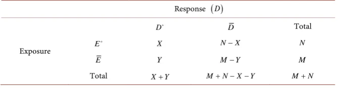
Table 2. Disease-exposure cross classification in a 2 × 2 table.

Response

( )

D

D+ D Total

Exposure E

+ _{X N}−_{X N}

E Y M−Y M

given by:



(

)

(

)

(

)

.

X M Y Y N X

AR

X Y M

− − −

=

+ (5)

Following [9], we shall derive the asymptotic variance of _θˆ_{=ln 1}

(

₋_AR

)

_.

We first write, Var

( )

X =NP

(

1−P c

)

1, and, Var

( )

Y =MQ

(

1−Q c

)

2,

where c1= +1

(

n0−1

)

ρ1, c2 = +1

(

m0−1

)

ρ2,

2

0 1

k i i

n =

∑

₌n N, and 2

0 1

l i i

m =

∑

₌m M .

Using the delta method [10] we can show to the first order of approximation that:

( )

₍

(

)

₎

2

(

₍

)

₎

1 2

2 2

1 1

Var N P C N P C .

P N M MP N M

θ = − + − Ψ

+ Ψ Ψ + Ψ



(6)

A consistent estimator of Var

( )

θ may be obtained on replacing the para-

meters P c c, ,1 2 and Ψ by their moment estimators. An

(

1−α

)

100% confi-dence interval on AR is thus given as:

( )

(

)

(

( )

)

(

1 exp− θ +zα2 var θ ,1 exp− θ −zα2 var θ

)

.

   

The moment estimators of the intraclass correlations are obtained separately from the groups of exposed and unexposed clusters. The moment estimator of

1

ρ is given by:

(

)

1 0 ˆ 1 MSB MSW

MSB n MSW

ρ = −

+ − (7)

where r,

(

)

1 1

1 k n_i ij ij ij

i j

ij

x n x

MSW

n k = = n

− =

−

∑ ∑

(8)

(

)

2

1 1

1

. 1

i ij i

k n i j

ij

x x

MSB

k = = n

− =

−

∑ ∑

(9)

Similar expressions for the (MSW, MSB) are obtained for the clusters of un-exposed. The quantities (MSW, MSB) are estimated from the one-way ANOVA model when the responses are measured on the binary scale. For details the readers are referred to [6].

We now consider two examples, the first is from data arising from a cross sec-tional study and the second example is on data from a randomized prospective trial.

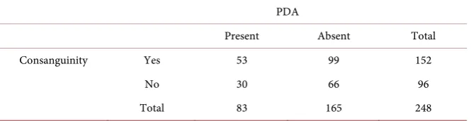
Example 1: Cross-Sectional Study: The effect of consanguinity on congenital heart defects (CHD).

The participating hospitals are from regions that cover the country making the registry a nationwide data repository for the Kingdom of Saudi Arabia [Con-genital Heart Disease Registry 2013]. The present example uses data on a major congenital heart disease; Patent Ductus Arteriosus (PDA). The incidence of PDA has been reported to be approximately, 1 in 2000 births, which accounts for 5% to 10% of all congenital heart diseases with female to male ratio of almost 2:1 [12]. The PDA was found to occur with increased frequency in several genetic syndromes, with precise mechanisms resulting in persistent PDA not yet clear [13][14].

Arab countries are notorious for consanguineous marriages, with first cousin types being the most common. For example in Jordan the prevalence of consan-guinity was reported in [15] as 51.3%, Yemen, 40% as reported [16], and almost 57% in Saudi Arabia as reported [17][18]. More recently, a survey of Saudi fam-ilies conducted in [19], estimated the prevalence of consanguinity to be as high as 56%.

For illustrative purposes of the methodologies presented in this section, we sampled two children from the registry whose mother are non-diabetic, with ma-ternal age less than 40 years. Each sampled child was classified according to the presence/absence of PDA, and the type of parental consanguinity (exposure varia-ble). Therefore, for the exposed (children from consanguineous marriages re-stricted to first degree cousin) and non-exposed (children from non-consangui- neous marriages) the cluster size is n= =m 2. The data are presented in Table 3.

Direct applications using Equations (5), (8), (9), and (10) we get:

( )( ) ( )( )

( )( )

53 66 30 99

AR 6.6%

83 96

−

= = _, P E

( )

=0.61

1 0.325

ρ = _, ρ =₂ 0.332, P=P Dr

(

Consanguineous

)

=0.39,

(

)

0.349

Non Consanguineous 0.31, and 1.11 0.313

r

Q=P D − = RR= = .

The square root of Equation (6) gives _se

( )

_{θ =}ˆ _{0.085, and the 95% confidence}

interval of AR is: −0.104 < AR < 0.210.

The AR estimate is interpreted as follow: if among infants born with CHD, gi- ven that PDA among infants with CHD is a preventable event, then prohibiting first degree relatives’ marriages will reduce the chance of having PDA by 6%.

Example 2: Prospective Cohort study (Weil’s data)

[image:6.595.208.541.647.733.2]

The data in this example was given first in [20] taken from [21], and gives the

Table 3. Consanguinity and PDA.

PDA

Present Absent Total

Consanguinity Yes 53 99 152

No 30 66 96

results from an experiment comparing two treatments. One group of 16 preg-nant female rats was fed a control diet during pregnancy and lactation, while the diet of a second group of 16 pregnant females was treated with a chemical. For each cluster (litter consisting of the pups born to a female rat), the number n of pups alive at 4 days and the number y of pups that survived at 31 day lactation period were recorded. The data are given as a fraction y n in Table 4.

In Table 4, the numerator is the number of dead pups during 21 days lacta-tion period, and the numerator is the number who survived past 4 days. The pur-pose of the experiment was to determine if the chemical treatment significantly affects the survival rate among the pups. That is, we need to test the null hypo-thesis H0:P=Q. The data are presented in a 2 × 2 format in Table 5.

0.24

P= and Q=0.10, giving relative risk RR=2.4.

( )( ) ( )( )

( )( )

35 142 16 112

39.4%. 51 158

AR= − =

(

control

)

0.029

ρ = _, ρ

(

treated

)

=0.040, n₀=9.84, m0 =9.16, and

( )

ˆ _0.0555

se θ = , and the 95% confidence interval on AR is: 0.33 < AR < 0.45.

3. Split Cluster Design

Split-cluster experiments are being used by investigators in health sciences when naturally occurring aggregates of individuals with nested subgroups may be as-signed to different treatments. Cited examples include split mouth trials, in which a subject’s mouth is divided into two segments that are randomly assigned to different treatment groups. In other situation, randomization to treatment conditions may be possible at the person level within the cluster. In this case, when the treatment conditions are available within each cluster, the design is re-ferred to as a multisite or split cluster design (SCD). The major attractiveness of this design is that it removes a large portion of the inter-subject variation from the estimate of treatment effect; and hence has the potential to require a lesser number of subjects than a parallel arm design with the same power. When the response variable of interest is binary, statistical methods developed to evaluate the effect of intervention depends on non-parametric methods, as shown in [22].

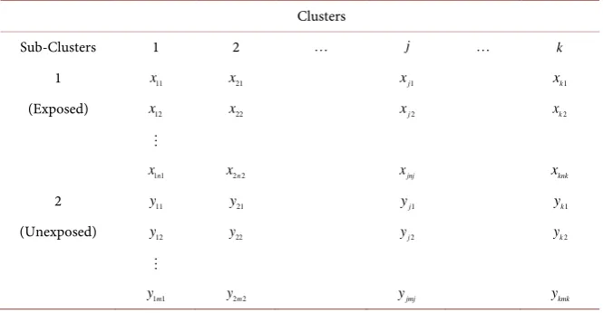
In this section we present the data layout for the SCD (see Table 6) and derive the large sample variance of the AR as a measure of effect size.

Under a similar set up to that we presented in the previous section and with appropriate change in notations the random variables 1

i

n i j ij

X =

∑

₌ x and

1

i

m i j ij

[image:7.595.210.537.670.732.2]

Y =

∑

₌ y will have the same beta-binomial distributions, but they are no- longer independent.

Table 4. Weil’s data: Mortality due to exposure is a two arms clinical trial.

Control 13/13 12/12 9/9 9/9 8/8 8/8 12/13 11/12

9/10 9/10 8/9 11/13 4/5 5/7 7/10 7/10

Treatment 12/12 11/11 10/10 9/9 10/11 9/11 9/11 8/9

[image:8.595.209.538.90.169.2]

Table 5. Weil’s data collapsed in a 2 × 2 table.

Exposure Status Total

Dead Alive

Treated 35 112 147

Control 16 142 158

Total 51 254 305

Table 6. Data layout for the split-cluster design.

Clusters

Sub-Clusters 1 2  j _ k

1 x11 x21 xj1 xk1

(Exposed) x12 x22 xj2 xk2



1 1n

x x_{2 2n} x_jnj x_knk

2 y11 y21 yj1 yk1

(Unexposed) y12 y22 yj2 yk2



1 1m

y y_{2 2m} y_jmj y_kmk

( )

(

)

(

1

)

1

Var X =NP 1−P _1+ u −1

ρ

_

( )

(

)

(

2

)

2

Var Y =MQ 1−Q _1+ u −1

ρ

_.

The correlation parameters ρ1 and ρ2 are estimated as shown in Equations (7)-(9).

Although the AR estimator maintains the same expression under split clusters, its variance is affected by the correlations within the sub-clusters, and between units in the exposed and the non-exposed sub-clusters.

Using the delta method, we can therefore show that

( )

_[

(

)

_]

(

_[

)

_]

[

]

(

)(

)

2

1 2

2 2

1 2 12

1 2 2

1 1

ˆ Var

2

1 1

N P c N P c

P N M M P N M

NP

NM P P c c

M P N M

ψ θ

ψ ψ ψ

ρ _{ψ ψ}

ψ ψ

− −

= +

+ +

−

+_ _ − − _ _

 + 

 

(10)

where c1= +1

(

u1−1

)

ρ1, c2 = +1

(

u2−1

)

ρ2,

2

1 1

k i i

u =

∑

₌n N and

2

2 1

k i i

u =

∑

₌ m M .

[image:8.595.207.540.201.374.2]

then use the one-way ANOVA to obtain the within and between mean squares. Substituting these quantities in (7) we obtain a moment estimator of ρ12.

Example 3: Split-Mouth Trial

For illustrating the proposed methodology, as a third example, we consider data from a split-mouth trial on 23 patients evaluating the effect of chlorhex-idine in the treatment of gingivitis [22]. The data are presented in Table 7. The chlorhexidine and control treatments were randomly applied to four sites lo-cated in the patient’s left and right sides of the upper and lower jaws. We are in-terested here in testing the effect of treatment on the presence or absence of plaque, as based on the measurements taken two weeks after baseline and sum-marized in Table 8. The sample estimates and standard errors (SE) of P and Q, the proportion of patients having plaque in the chlorhexidine and control groups, are estimated at 0.89 (SE = 0.0343), and 0.77 (SE = 0.0491), respectively. The intra-class and inter-class correlation coefficients are estimated as

1

ˆ 0.0395

ρ = , ρ =ˆ2 0.087, as shown in the previous section, pooled estimate

ˆ 0.070

ρ = _{The sample estimate of the relative risk RR is 1.155.}

1 0.0395

ρ = _, ρ =₂ 0.087, ρ =12 0.039.

( )( ) ( )( )

( )( )

82 21 10 71 1722 710

7.19%. 153 92 14076

AR= − = − =

( )

ˆ _0.092

se θ = , and the 95% CI on AR is (−0.112, 0.225).

4. Testing the Equality of Two Correlated

AR

Parameters

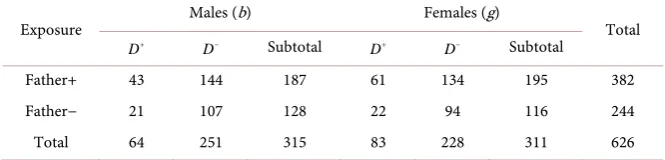
Interest is focused on studying the change in disease-exposure etiology under va- rying conditions. We illustrate this situation using the published data [23].

[image:9.595.207.539.543.606.2]

For example in the case of family data we may be interested in evaluating the effect of disease status of a parental exposure variable on their siblings, which can be divided into males and females within the same family. In this case, we

Table 7. Number of sites with plaque in four sites

(

m_ij=4

)

treated with chlorhexidine and control in 23. The data are adapted from [22] and is given in Table 7.

Treat Affected (+) Not Affected (−) Total

Chloro. (1) 82 10 92

Control (2) 71 21 92

Total 153 31 184

Table 8. Disease distribution among males and females according to father (exposure va-riable) disease status.

Exposure Males (b) Females (g) Total

D+ D− Subtotal D+ D− Subtotal

Father+ 43 144 187 61 134 195 382

Father− 21 107 128 22 94 116 244

[image:9.595.206.539.652.732.2]

have two correlated attributable risk estimator, one describing the disease-ex- pose etiology for males, and the other for females. The main interest here is to compare the AR of males to that of females from the same sib-ship.

Example 4: Correlated AR’s from Cross Sectional Study: Family Data We now consider a highly structured clustered familial data that has a two level hierarchy with blood measurements taken on parents (level two) and their offspring (level one) together with other anthropometric features [23]. Familial data sets are known to have considerable “within-cluster” correlation due to the homogeneous nature of family members. The goal is to classify the offspring blood pressure status based on parents BP and other anthropometric features. The data set contains 223 families with a mean number of siblings equal to 3 siblings per family. The outcome variable in this data set is a binary variable de-fined as offspring blood pressure status. If simultaneously SBP > 130 and DBP > 80, then an offspring is considered diseased

( )

D+ or otherwise normal

( )

D− . The exposure variable in this example is whether a parent (here we select the fa-ther) has the condition (presence of exposure) or does not have the condition (absence of exposure). The data are presented in Table 8.

We present the general methodology as follows: Testing for gender difference in the population AR is formulated as testing the null hypothesis

0: 1 2

H AR = AR against a general unspecified alternative H1:AR2=AR1+ ∆. Note that testing this null hypothesis is equivalent to testing

0: 1 2, or 0: 0

H θ θ= H ∆ = .

Let the point estimators be denoted by θˆ1 and θˆ2. The difference

1 2

ˆ ˆ

D=θ θ− is asymptotically unbiased and has variance

( )

( )

ˆ1

( )

ˆ2

( )

ˆ ˆ1 2

var D =var θ +var θ −2 cov θ θ, .

Hence the null hypothesis is rejected whenever Z =D var

( )

D falls in the interval Z>zα2 or Z< −zα2 , where zα2 is the

(

1−α 2 100%

)

cut off

point on the standard normal curve. With a slight difference in notation,

( )

ˆ

var θi is similar to the expression in Equation (6). We derive cov

(

θ θˆ ˆ1, 2

)

using the delta method. In general, the data will have a structure similar to that given in Table 9.

We define the moment estimator as before:



(

) (

)

(

)

1, 2.

j j j j j j

j

j j j

x M Y Y N X

AR j

M X Y

− − −

= =

+

Let ˆ _{ln 1}

(

_j

)

j AR

θ = − _{, then similar to the first situation, we have:}

( )

₍

(

)

₎

2

(

₍

)

₎

1 2

2

2 2

1 1

ˆ

var j j j j j j j .

j j

j j j j j j j j j j

N P c N P c

P N M M P N M

ψ

τ θ

ψ ψ ψ

− −

= = +

[image:10.595.206.540.677.735.2]

+ +

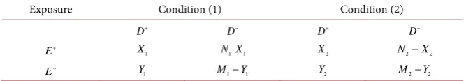
Table 9. Collapsed data for the analysis of correlated AR parameters.

Exposure Condition (1) Condition (2)

D+ D− D+ D−

E+ X1 N X1− 1 X2 N2−X2

Here;

1

j

k j i ji

N =

∑

₌ n , lj₁

j i ji

M =

∑

₌m , c1j = +1

(

n0j−1

)

ρ

1j, c2j = +1

(

m0j −1

)

ρ

2j,

and 2

0 1

1 kj

j i ji

j

n n

N =

=

∑

_, 2

(

) (

)

0 1

1

, 1 1

j

l

j i ji j j j

j

m m AR AR

M = ψ

=

∑

= − + _{, and}

rate of exposure to the risk factor under the condition

j

P = jth .

Moreover, ρ1j is the intracluster correlation of the exposed clusters under jth condition, and ρ_2j is the intracluster correlation of the unexposed clus-ters under jth condition. They two parameters are estimated as described in (7).

For simplicity we assume that these correlations are constant among the ex-posed and unexex-posed.

Using the delta method we can show after some algebra that:

( )

ˆ ˆ1 2

[

1 2 1 2 2 1 2 1 1 2 1 2 1 2 1 2

]

cov θ θ, =ρ α α γ γ +α β γ δ α β γ δ+ +β β δ δ .

(11)

The correlation

ρ

which, under both conditions is the average correlation among the responses, is estimated as described in Section 3.

The values inside the square bracket are given by:

(

1

)

j j

j j j j j

x P N M

θ α ψ ∂ = = − ∂ +

(

)

j j j

j j j j j j j

N

y M P N M

θ β ψ ψ ∂ = = − ∂ +

( )

(

)

2 1 var 1

j xj N Pj j P cj j

γ

= = −

( )

(

)

(

)

2 2 2 var 1

1 1, 2.

j j j j j j

j j j j j j

y M Q Q c

M P P c j

δ

ψ ψ

= = −

= − =

Therefore;

(

)

2 2

[

]

1 2 1 2 1 2 1 2 2 1 2 1 1 2 1 2 1 2 1 2

ˆ ˆ

var θ θ− =τ +τ −2ρ α α γ γ +α β γ δ α β γ δ β β δ δ+ + .

(12)

Using the data in Table 8 we get:

Males: P1=.59, M1=128,AR1=.19, var

( )

θ =ˆ1 .0142. Females:P2 =.63, M2 =244,AR2 =.29, var

( )

θ =ˆ2 .00578

(

ˆ1 ˆ2

)

var θ θ− =.01987, .211 .342 0.929

.141

z=− + = , and p−value=0.353.

Therefore there is not enough evidence in the data to support the hypothesis of presence of gender differences for the paternal effect on the siblings’ hyper-tension status.

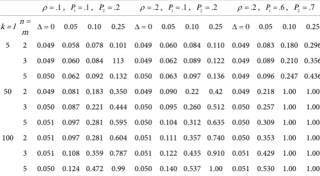
5. Simulations

number of scenarios under which we examine the properties of the proposed test statistic Z. The statistic Z =D var

( )

D is computed when both P₁ and P2 are strictly positive with additional restriction,

(

2 2

)

[

]

1 2 2 1 2 1 2 2 1 2 1 1 2 1 2 1 2 1 2

ρ

<

τ

+

τ

α α γ γ

+

α β γ δ α β γ δ

+ +

β β δ δ

_{. If these conditions}

are not satisfied, the sample is replaced until a total of 1000 iterations are ob-tained for each parameter combination. Table 10 shows the empirical levels and powers of the test assuming that the number of clusters is the same under both conditions and for the exposed and the non-exposed clusters. The main conclu-sions from Table 10, is that the proposed test statistic hold its empirical Type I error rate levels. There is an increase in the test power when the correlation in-creases, and when the prevalence of exposure parameters P1 and P2 are away from the boundaries of the interval (0, 1). We also note an appreciate increase in the power when the number of clusters is above 50, and naturally when the tested parameters are well separated.

6. Discussion

The population Attributable risk, like the odds ratio and relative risk is a meas-ure of disease risk association. However it has a special appeal to public health epidemiologists as it measures the percent reduction in the chances of having the outcome among subjects who are exposed to the risk factor. Clearly, not every-one in the population is exposed to the risk factor. For example, in evaluating the relationship between consanguinity and the risk of PDA, not all parents are relatives. We assume say that 55% of women in the population (as in the Saudi traditional society) are married to a first cousin. To determine how much of a reduction there would be in PDA among CHD newborns we have 0.55 × 0.06 = 3.3%.

We have developed estimators of the variance and the confidence interval on

[image:12.595.209.533.555.733.2]

AR when the units of sampling are aggregates of individuals under three study designs. In all situations the estimation of the intraclass correlation is crucial to

Table 10. Empirical type i error rates and powers based on 1000 replications from the bi-variate beta binomial distribution. We set AR1 = 0.05, and therefore, AR2=AR1− ∆.

.1

ρ = , P1=.1, P2=.2 ρ =.2, P1=.1, P2=.2 ρ =.2, P1=.6, P2=.7

k = l n = _m ∆ =0 0.05 0.10 0.25 ∆ =0 0.05 0.10 0.25 ∆ =0 0.05 0.10 0.25

conduct valid statistical inferences.

One of the objectives of this paper was to develop and evaluate simple test sta-tistic that could be used to compare dependent attributable risks in the case of clustered dichotomous outcome variables.

7. Conclusions

1) Through simulations, a major finding of our work is that to test the equality of correlated attributable risks, either from cross sectional or cohort studies, one needs a much larger number of clusters than that expected to achieve high power. 2) An interesting extension of our study is to construct model-based inference on the AR. This would require the development of a semi parametric model sim-ilar to the generalized estimating equation, or a full probabilistic model such as generalized linear mixed model where the effect of multiple covariates may be accounted for.

3) A limitation of the simulation study is the restrictions that the number of observations in all clusters is held constant (balanced design) and that the within cluster and the cross cluster correlations are equal. The reason for this assump-tion is to limit the number of factors which affect the power so that reasonable conclusions can be made. But we believe that these restrictions should not affect the overall conclusions.

Conflict of Interest

The authors declare that there is no conflict of interest.

References

[1] Richardson, J. (1996) Measures of Effect Size. Behavior Research Methods, Instru-ments and Computers, 28, 12-22. https://doi.org/10.3758/BF03203631

[2] Levin, M.L. (1953) The Occurrence of Lung Cancer In Man. Acta Unio Internatio-nalis Contra Cancrum, 9, 531-541.

[3] Fleiss, J. (1982) Statistical Methods for Rates and Proportions. 2nd Edition, John Wiley, New York.

[4] Fletcher, R.H., Fletcher, S.W. and Wagner, E.H. (1996) Clinical Epidemiology: The Essentials. Lippincott Williams & Wilkins, Philadelphia.

[5] Gordis, L. (1996)Epidemiology. WB Saunders Co., Philadelphia.

[6] Donner, A. and Klar, N. (2000) Design and Analysis of Cluster Randomized Trials in Health Research. Arnold, New York.

[7] McCullagh, P. and Nelder, J.A. (1989) Generalized Linear Models. 2nd Edition, Chapman & Hall/CRC.

[8] Cox, D.R. and Snell, E.J. (1989) Analysis of Binary Data. 2nd Edition, CRC Press, Boca Raton, FL.

[9] Walter, S.D. (1975) The Distribution of Levin’s Measure of Attributable Risk from Case-Control Studies. American Journal of Epidemiology, 106, 206.

[10] Kendall, M. and Stuart, A. (1987) Advanced Theory of Statistics. Vol. 1, 5th Edition, Griffin, London.

[12] Mitchell, S.C., Korones, S.B. and Berendes, H.W. (1971) Congenital Heart Disease, in 56,109 Births. Incidence and Natural History. Circulation, 43, 323-332.

https://doi.org/10.1161/01.CIR.43.3.323

[13] Satoda, M., Pierpont, M.E., Diaz, G.A., Bornemeier, R.A. and Gelb, B.D. (1999) Char Syndrome, an Inherited Disorder with Patent Ductus Arteriosus, Maps to Chromosome 6p12-p21. Circulation,99, 3036-3042.

https://doi.org/10.1161/01.CIR.99.23.3036

[14] Satoda, M., Zhao, F., Diaz, G.A., Burn, J., Goodship, J., Davidson, H.R., Pierpont, M.E. and Gelb, B.D. (2000) Mutations in TFAP2B Cause Char Syndrome, a Familial Form of Patent Ductus Arteriosus. Nature Genetics, 25, 42-46.

https://doi.org/10.1038/75578

[15] Khoury, S.A. and Massad, D. (1992) Consanguineous Marriages in Jordan. Ameri-can Journal of Medical Genetics, 43, 769-775.

https://doi.org/10.1002/ajmg.1320430502

[16] Jurdi, R. and Saxena, P.C. (2003) The Prevalence and Correlates of Consanguineous Marriages in Yemen: Similarities and Correlates with Other Arab Countries. Jour-nal of Biosocial Sciences,35, 1-13. https://doi.org/10.1017/S0021932003000014

[17] El-Hazmi, M.A., Al-Swailem, A.R. and Warsey, A.S. (1995) Consanguinity among the Saudi Arabian Population. Journal of Medical Genetics, 32, 623-626.

https://doi.org/10.1136/jmg.32.8.623

[18] Becker, S.M., Al Halees, Z., Molina, C. and Paterson, R.M. (2001) Consanguinity and Congenital Heart Disease in Saudi Arabia. American Journal of Medical Genet-ics Part A, 99, 8-13.

https://doi.org/10.1002/1096-8628(20010215)99:1<8::AID-AJMG1116>3.0.CO;2-U

[19] El-Mouzan, M., Al-Salloum, A., Al-Herbish, A., Qurashi, M. and Al-Omar, A. (2008) Consanguinity and Major Genetic Disorders in Saudi Children: A Commu-nity-Based Cross-Sectional Study. Annals of Saudi Medicine, 28, 169-174.

https://doi.org/10.4103/0256-4947.51726

[20] William, D.A. (1975) The Analysis of Binary Responses from Toxicological Experi-ments Involving Reproduction and Teratogenicity. Biometrics, 31, 949-952.

https://doi.org/10.2307/2529820

[21] Weil, C.S. (1971) Selection of the Valid Number of Sampling Units and a Consider-ation of Their CombinConsider-ation in Toxicological Studies Involving Reproduction, Te-ratogenesis or Carcinogenesis. Food Cosmetics Toxicology, 8, 177-182.

[22] Donner, A., Klar, N. and Zou, G. (2004) Methods for the Statistical Analysis of Bi-nary Data in Split-Cluster Designs. Biometrics,60, 919-925.

https://doi.org/10.1111/j.0006-341X.2004.00247.x

Submit or recommend next manuscript to SCIRP and we will provide best service for you:

Accepting pre-submission inquiries through Email, Facebook, LinkedIn, Twitter, etc. A wide selection of journals (inclusive of 9 subjects, more than 200 journals)

Providing 24-hour high-quality service User-friendly online submission system Fair and swift peer-review system

Efficient typesetting and proofreading procedure

Display of the result of downloads and visits, as well as the number of cited articles Maximum dissemination of your research work