Grid integration and smart grid
implementation of emerging technologies
in electric power systems through
approximate dynamic programming
Xiao, Jingjie
Purdue University
13 August 2013
Online at
https://mpra.ub.uni-muenchen.de/58696/
EMERGING TECHNOLOGIES IN ELECTRIC POWER SYSTEMS THROUGH
APPROXIMATE DYNAMIC PROGRAMMING
A Dissertation
Submitted to the Faculty
of
Purdue University
by
Jingjie Xiao
In Partial Fulfillment of the
Requirements for the Degree
of
Doctor of Philosophy
December 2013
Purdue University
ACKNOWLEDGMENTS
I would like to thank my advisors, Dr. Joseph Pekny and Dr. Andrew Liu,
for their guidance, insight, patience, and trust, and for always being inspiring and
supportive. I would also like to thank them for the freedom they gave me to pursue
my own interests.
I would also like to thank my committee members, Dr. James Dietz and Dr. Omid
Nohadani for sharing their expertise, and giving me advice and encouragement. To
Dr. Gintaras Reklaitis for sharing his knowledge and being supportive.
I could never have finished without the help of my group-mates and collaborators:
Dr. Bri-Mathias Hodge, Dr. Shisheng Huang, Xiaohui Liu, and Hameed Safiullah.
I were lucky to work with them and have them as good friends. To my office-mates
and good friends: Dr. Ye Chen, Manasa Ganoothula, Elcin Icten, Harikrishnan
Sreekumaran, Emrah Ozkaya, Anshu Gupta, and Aviral Shukla who made the office
a productive and entertaining place.
TABLE OF CONTENTS
Page
LIST OF TABLES . . . v
LIST OF FIGURES . . . vi
ABSTRACT . . . viii
1 INTRODUCTION . . . 1
1.1 Motivation and Literature Review . . . 1
1.2 Research Objectives and Contributions . . . 9
1.3 Technical Background . . . 11
1.3.1 Dynamic programming . . . 11
1.3.2 Approximate dynamic programming . . . 14
2 CENTRALIZED PLUG-IN HYBRID ELECTRIC VEHICLE CHARGING 18 2.1 Outline of the Short-Term Energy System Model . . . 18
2.2 A Deterministic Linear Programming Formulation . . . 21
2.3 An Approximate Dynamic Programming Formulation . . . 24
2.3.1 Making decisions approximately . . . 27
2.3.2 Value function approximation . . . 28
2.3.3 Complete algorithm. . . 32
2.4 Test Case: the California System . . . 33
2.4.1 Electricity Demand . . . 34
2.4.2 Electricity Generation . . . 35
2.4.3 Modeling and Forecasting Wind Power . . . 38
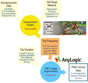
2.4.4 Obtaining PHEV Arrival Rate . . . 40
2.5 Evaluating Approximate Dynamic Programming Solutions . . . 45
2.5.1 Performance measures under deterministic assumption . . . 46
Page
2.5.3 Selecting step size . . . 53
3 EXTENSIONS OF THE SHORT-TERM ENERGY SYSTEM MODEL . 58 3.1 Decentralized PHEV Charging . . . 58
3.1.1 A deterministic mixed integer linear programming formulation 59 3.1.2 An approximate dynamic programming formulation . . . 60
3.2 Decentralized PHEV Charging with Vehicle-to-Grid as Storage . . . 63
3.2.1 A deterministic mixed integer linear programming formulation 64 3.2.2 An approximate dynamic programming formulation . . . 66
3.3 Comparing PHEV Charging Policies . . . 70
4 RESOURCE PLANNING WITH REAL-TIME PRICING . . . 77
4.1 Outline of the Long-Term Energy System Model . . . 78
4.2 A Deterministic Linear Programming Formulation . . . 81
4.3 An Approximate Dynamic Programming Formulation . . . 83
4.4 Numerical Results. . . 87
5 CONCLUSIONS AND FUTURE WORK . . . 91
LIST OF REFERENCES . . . 94
A MATLAB CODES . . . 102
LIST OF TABLES
Table Page
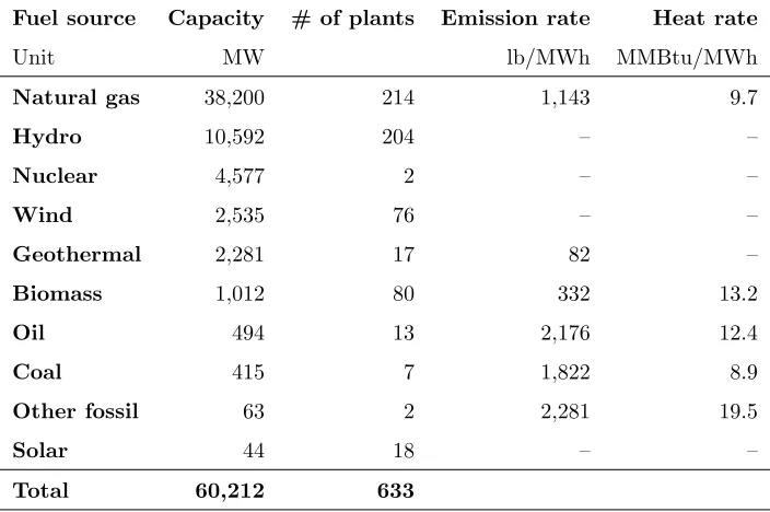
2.1 Statistics for the electric power generation by fuel type, California, 2009 35
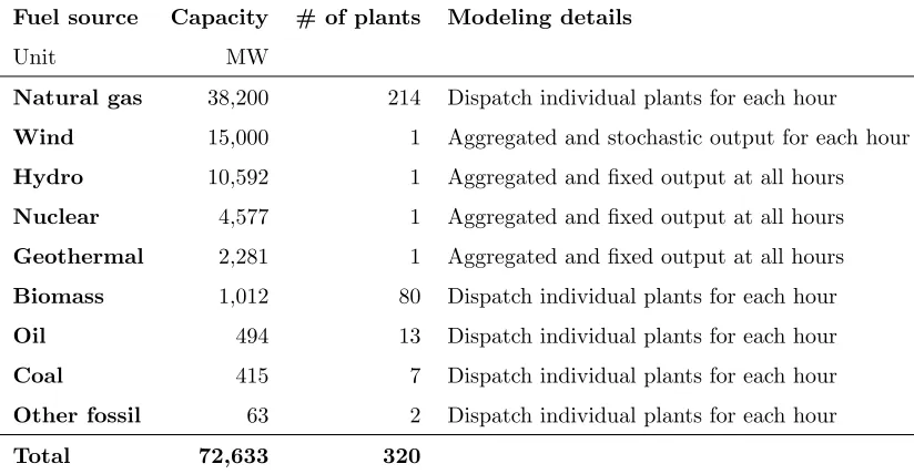
2.2 Modeling the electric power generation by fuel type . . . 37
2.3 Characteristics of the California transportation system (BTS) . . . 45
2.4 Characteristics of Chevrolet Volt (EPA) . . . 45
2.5 Characteristics of various charging configurations [89] . . . 45
2.6 Performance statistics of the ADP algorithm for deterministic cases under different PHEV penetration rates . . . 47
2.7 Performance statistics of the ADP algorithm for stochastic cases under different PHEV penetration rates . . . 52
2.8 Performance statistics of the ADP algorithm for stochastic cases under dif-ferent PHEV penetration rates (with an increased variance in wind forecast error) . . . 52
4.1 Costs comparison for various charging policies . . . 90
LIST OF FIGURES
Figure Page
1.1 Overview of implementing approximate dynamic programming . . . . 15
2.1 Illustrating a PHEVs’ charging due time given its arrival time . . . 23
2.2 Computing the electricity consumed for charging PHEVs at each hour in a day . . . 23
2.3 Illustrating how to obtain a new sample estimate of the value function gradient approximation given the wholesale electricity price approximations 31
2.4 Statistics of system demand at different hours in a day, California, August 2009 . . . 34
2.5 Statistics for electric power generation mix using a bubble chart, Califor-nia, 2009 . . . 36
2.6 Statistics of wind availability factor at different hour in a day, California, August 2006 . . . 39
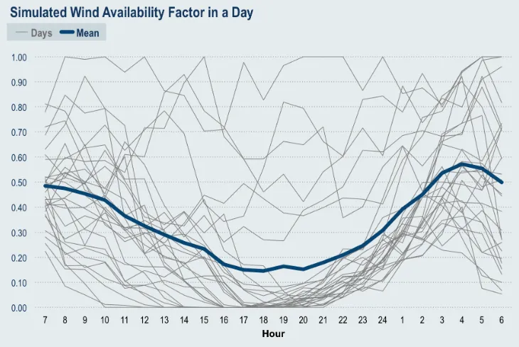
2.7 Plot of simulated wind availability factor at different hour in a day, Cali-fornia, August . . . 41
2.8 Flowchart overview of modeling PHEV arrival at different hour in a day 42
2.9 Probability that a PHEV is plugged in at different hour in a day . . . . 43
2.10 Optimal PHEV charging decision fromOP T andADP for a deterministic case . . . 48
2.11 Optimal PHEV charging decision in a day from ADP and W S for a stochastic case . . . 50
2.12 Hourly electricity demand in a day from OP T and ADP for a stochastic case . . . 51
2.13 Hourly wholesale electricity price in a day from OP T and ADP for a stochastic case . . . 51
2.14 Plot of the objective values with respect to iterationnfor step size (0.3, 0.1), for a deterministic case . . . 54
Figure Page
2.16 Plot of the objective values with respect to iterationnfor step size (0.5, 0.1), for a stochastic case . . . 55
2.17 Plot of the objective values with respect to iterationnfor step size (1/n, 0.2), for a stochastic case . . . 55
2.18 Choosing the best step size based on the mean and standard deviation of the objective values generated by the ADP algorithm . . . 56
3.1 Illustrating how to generation a new estimate of marginal value of in-creasing PHEV inventory by one unit, given wholesale electricity price approximations . . . 69
3.2 System demand profile in a day under four charging scenarios . . . 72
3.3 Wholesale electricity price profile in a day under four charging scenarios 72
3.4 Generation costs in a day for four charging scenarios and five PHEV pen-etration levels . . . 73
3.5 Generator emissions in a day for four charging scenarios and five PHEV penetration levels . . . 73
3.6 Consumers’ electric payment in a day for four charging scenarios and five PHEV penetration levels . . . 74
3.7 Generator and tailpipe emissions in a day, assuming a high tailpipe emis-sion rate . . . 74
3.8 Generator and tailpipe emissions in a day, assuming a low tailpipe emission rate . . . 75
4.1 Wind capacity investment decision under different pricing and charging schemes . . . 88
ABSTRACT
Xiao, Jingjie Ph.D., Purdue University, December 2013. Grid Integration and Smart Grid Implementation of Emerging Technologies in Electric Power Systems Through Approximate Dynamic Programming. Major Professor: Joseph F. Pekny and An-drew L. Liu.
A key hurdle for implementing real-time pricing of electricity is a lack of
con-sumers’ responses. Solutions to overcome the hurdle include the energy management
system that automatically optimizes household appliance usage such as plug-in hybrid
electric vehicle charging (and discharging with vehicle-to-grid) via a two-way
com-munication with the grid. Real-time pricing, combined with household automation
devices, has a potential to accommodate an increasing penetration of plug-in hybrid
electric vehicles. In addition, the intelligent energy controller on the consumer-side
can help increase the utilization rate of the intermittent renewable resource, as the
demand can be managed to match the output profile of renewables, thus making the
intermittent resource such as wind and solar more economically competitive in the
long run.
One of the main goals of this dissertation is to present how real-time retail pricing,
aided by control automation devices, can be integrated into the wholesale
electric-ity market under various uncertainties through approximate dynamic programming.
What distinguishes this study from the existing work in the literature is that
whole-sale electricity prices are endogenously determined as we solve a system operator’s
economic dispatch problem on an hourly basis over the entire optimization horizon.
This modeling and algorithm framework will allow a feedback loop between
electric-ity prices and electricelectric-ity consumption to be fully captured. While we are interested
in a near-optimal solution using approximate dynamic programming; deterministic
The other goal of the dissertation is to use this framework to provide numerical
ev-idence to the debate on whether real-time pricing is superior than the current flat
rate structure in terms of both economic and environmental impacts. For this
pur-pose, the modeling and algorithm framework is tested on a large-scale test case with
hundreds of power plants based on data available for California, making our findings
useful for policy makers, system operators and utility companies to gain a concrete
1. INTRODUCTION
1.1 Motivation and Literature Review
The retail electricity rate has been kept flat for the past century, mainly due
to technological limitations and regulatory policies. On the other hand, wholesale
electricity prices vary constantly (e.g. hourly, or even minute-by-minute) to reflect
changes in costs of producing electricity at different time. It has long been understood
that the current flat retail rate structure is inefficient [1–5]. It prevents consumers
from benefitting from a lower electricity bill by reducing their electricity consumption
when the wholesale electricity price is high and increasing their consumption during
time periods when the electricity price is low. An inelastic short-term demand,
com-bined with extremely high costs of blackouts [6–8], also means that sufficient
generat-ing capacity must be installed to satisfy some extreme realizations of demand shocks.
This leads to an electricity system that is overly built with capital intensive assets,
solely to maintain system reliability.
Aware of potential benefits of demand-side participation, the U.S. Department of
Energy (DOE) envisions a future electricity system, referred to as Smart Grid [9–13],
where consumers are fully integrated into wholesale power markets. The Federal
Energy Regulatory Commission (FERC) also encourages a wholesale market where
demand and supply are treated symmetrically. How are the visions of smart grid
to be implemented, however, is still a subject of a great deal of debate [14–18].
Programs intended to promote demand-side participation can be divided into two
major categories: incentive-based demand response (DR) programs, and time-varying
retail prices [19] including time-of-use tariffs (TOU), critical-peak pricing (CPP), and
Incentive-based demand response programs pay customers to reduce their
con-sumption relative to an admistratively set baseline level of concon-sumption. Studies
including Aalami et al. 2010 [20], Caron and Kesidis 2010 [21], and Parvania and
Fotuhi 2010 [22] focus on efficiently integrate such programs in wholesale electricity
markets to provide reserves. Time-varying prices can be static or dynamic. Static
time-varying prices, generally called time-of-use prices, are preset for pre-determined
hours and days; while dynamic prices are allowed to change on short notice, often
within a day or less. Important dynamic pricing schemes include real-time pricing
and critical peak pricing. Real-time pricing is characterized by passing on a price,
which best reflects changes in wholesale electricity prices and supply/demand
bal-ance, to consumers. Critical peak pricing allows for a retailer to occasionally declare
an unusually high retail price for a limited number of hours.
Economists have long recognized that dynamic pricing, reflecting varying system
conditions over locations as well as time, is the path to realizing full benefits of active
demand participation in the wholesale electricity market. For example, Borenstein
et al. 2002 [3] conclude that real-time pricing delivers the most benefits in terms of
reducing peak demand. Their conclusion is drawn based on a comprehensive
theo-retical and practical analysis of possible approaches to integrate an active demand
side into the wholesale electricity market. Hogan 2010 [5] also concludes in favor of
real-time pricing, but from a perspective of price signal development. He argues that
a straightforward way to implement real-time pricing is to use full wholesale
electric-ity prices, with a fixed customer charge for transmission and distribution, metering
and billing costs. However, to apply incentive-based demand response and critical
peak pricing, sophisticated calculations are required to achieve principles laid out by
FERC. Bushnell et al. 2009 [4] pinpoint an important drawback of using
incentive-based demand response. That is, individual customers will always know more about
their true baseline than the administrator of a demand response program. Therefore,
Despite its potential benefits, real-time pricing was not possible to implement in
the past because the meter that most consumers had can record only the sum of
con-sumption over each month, not in each minute or hour. However, these technological
limitations have been greatly reduced. For example, millions of smart meters that
record electricity consumption on frequent intervals have been installed.
Develop-ment of advanced metering infrastructure (AMI) has been increasingly encouraged
by federal and state incentives. AMI can enable a two-way communication between
consumers and electricity retailers (even a system operator1
) in terms of electricity
usages and prices [11, 24, 25].
Technologies such as AMI help pave an efficient path to universal deployment of
real-time pricing and active consumer participation. However, advanced
infrastruc-tures alone are not enough. There are at least two important barriers to a widespread
adoption of real-time pricing. The first barrier is a lack of knowledge among
con-sumers about how to respond to real-time updated prices. As most concon-sumers have
long been accustomed to a flat rate of electricity, it would take a long time for them to
learn to track and respond to dynamic electricity rates, if they decide to do so at all.
Allcott 2011 [1] has observed, based on the first real-time pricing program operated
in Chicago since 2003, that households rarely actively checked hourly prices provided
(via telephone or the Internet), as it was difficult for them to constantly monitor the
prices and respond properly. Andersen 2011 [26] also argues that business cases for
Smart Grid should work with or without consumers’ behavior change. Therefore,
without automation technologies, it would be difficult for consumers to respond to
real-time prices that change frequently.
To overcome this hurdle, enabling technologies that allow residential customers
to respond automatically to pricing signals without adding significant burden to
con-sumers’ lifestyle have emerged. Such metering and control systems, referred to as
household energy management controllers (EMCs) or energy management system
1A system operator is responsible for the operation of the electric grid to match demand and
(EMS), can be programmed to automatically optimize home appliances energy
us-age in response to real-time price signals. Existing products include GE NucleusR,
Control4R, etc. Some energy scheduling algorithms that can be embedded into EMCs
of a household or small business to maximize its utility (or minimize its energy cost)
have been desiged (Ibars et al. 2010 [27], Mohsenian-Rad et al. 2010 [28], etc).
The second barrier to a universal deployment of real-time pricing is political
resis-tance because of costs and risks associated with RTP. FERC 2009 [14] pinpoints the
disagreement on cost-benefit analysis of real-time pricing as one of regulatory barriers.
From a customer’s perspective, there are two main costs associated with time-varying
rates [19]. The first is the metering cost, which would be the cost of a smart meter
net of its operational benefit such as the avoided meter reading cost. The second
cost is the loss of welfare associated with reducing or shifting usage. There is no
consensus among the literature on the debate about whether real-time pricing would
have positive net welfare effects. For example, Allcott 2012 [2] estimates that
mov-ing from 10 percent of consumers on real-time pricmov-ing to 20 percent would increase
welfare in the PJM electricity market by $120 million per year in the long run. In
another study [1] based on a real-time pricing program in Chicago, the same author
concludes that households were not sufficiently price elastic to generate gains that
substantially outweigh the estimated cost of the advanced electricity meter required
to observe hourly consumption.
Another valid regulatory concern regarding real-time pricing of electricity is that
RTP could increase instability of the electric grid. For example, Allcott 2012 [2]
observes based on simulations that real-time pricing could cause peak energy prices
to increase, assuming that the reserve margin2
is a fixed percentage of peak demand.
He discovers that the reason behind this counter-intuitive observation is that the
required excess capacity is less with more consumers on RTP since the peak demand
with RTP is lower.
2Reserve margin must be imposed on the electric system to deal with some extreme realizations of
To address these regulatory concerns, we must show that real-time pricing could
yield tangible benefits to end consumers without facing significant volatility on their
monthly electric bills. One potential benefit from real-time pricing, aided with
house-hold automation devices, is that it can facilitate an increasing adoption of electric
vehicles (EVs) and/or plug-in hybrid electric vehicles (PHEVs). Interests in
devel-oping EV/PHEVs are driven by environmental concerns, and high and volatile fuel
prices [29]. While electric vehicles have a limited range and thus suffering from “range
anxiety” [30]; plug-in hybrid electric vehicles eliminate this problem as it has an
in-ternal combustion engine that works as a backup when its battery is depleted. In
this study, we use only PHEVs as an illustrative example. Adapting the modeling
framework to include EVs and other household appliances such as air conditioners
would be a straightforward extension.
The electricity consumed for charging PHEVs (e.g. 0.4 kW per mile driven for a
Chevy Volt) will present a significant new load on the existing electric system [31]. An
increased penetration of PHEVs will, if no additional measures are taken, increase
the system peak, since there is usually a natural coincidence between the normal
system peak and charging pattern. Thus, the uncoordinated new load associated
with charging will reduce the load factor3
and capacity utilization, increase peaking
generating unit usage, and raise electricity rates. It will also increase power losses
and voltage deviation [32], and reduce transformers’ life [33].
The impact of PHEVs on the electric grid depends on when they are charged.
From a PHEV owner’s point of view, their PHEV has to be charged overnight so
the driver can drive off in the morning with a fully-charged battery. This gives
op-portunities to strategically shift PHEV charging loads without causing inconvenience
to consumers. There is extensive literature on assessment of potential benefits of
coordinated charging on reducing the system demand peak, power losses, electricity
generation costs and emissions. In studies including Clement et al. 2009, 2010 [34,35],
3The load factor is defined as the average load divided by the peak load over a specified time
Denholm and Short 2006 [36], and Sortomme et al. 2011 [37], a system operator is
assumed to be able to directly control PHEV charging and to coordinate it with
power system operations. It is, however, unlikely for this scenario to be implemented
in the real world since it requires the system operator to track every PHEV in the
system. Besides the technological difficulty associated with such a centralized
charg-ing scenario, drivers’ privacy can also be a barrier in implementcharg-ing this scheme [38].
Although the centralized charging controlled by a system operator is not practical,
it can nonetheless serve as a benchmark case to which other more realistic charging
schemes can be compared. Thus, in this study the centralized charging scheme is
considered along with various other charging scenarios.
Some studies on PHEV charging argue that charging decisions should be left
to individual consumers, and time-varying tariffs can be provided as incentives for
consumers to shift their charging demand to late night hours when the electricity price
is low. A time-of-use tariff is used in Axsen et al. 2011 [39], Huang et al. 2011 [40],
and Parks et al. 2007 [41]. These studies are usually done through simulations (with
a detailed modeling of PHEV driving patterns) since it is trivial to determine the
start time of charging.
In this study, we are interested in using real-time pricing tariffs as signals to
coor-dinate PHEV charging. As we discussed early on, with the help of EMCs, residential
consumers will have the capability to effectively react to hourly-updated price signals
and optimize their charging start time. Studies including Conejo et al. 2010 [42], Han
et al. 2010 [43], Kishore and Snyder 2010 [44], and Valentine et al. 2011 [45] discuss
PHEV charging with a real-time pricing tariff. However, they treat price signals as
exogenous information and use historical wholesale electricity prices (or statistical
models based on historical data). By doing this, they assume that PHEV charging
demand does not affect the cost of generating electricity. This assumption does not
hold when the real-time price of electricity changes every hour or less. Real-time
pricing creates a closed feedback loop between electricity supply and demand, and
respect to the price in previous hours will influence the price in the upcoming
op-eration periods. Algorithms designed without considering this closed feedback loop
may not fully realize the benefit of deployment of real-time pricing. Mohsenian-Rad
and Leon-Garcia 2010 [46] argue that any residential energy management strategy in
hourly-updated real-time pricing requires price prediction capabilities. A few
stud-ies share this view and examine decentralized charging, in which charging decisions
are made on residential level in response to real-time pricing, based on convex
op-timization (Samadi et al. 2010 [47]), mixed integer linear programming (Sioshansi
2012 [48]), dynamic programming (Livengood and Larson 2009 [49]), reinforcement
learning (O’Neill et al. 2010 [50]), game theory (Chen et al. 2011 [51], Mohsenian-Rad
and Leon-Garcia 2010 [46]). Our work is distinguish from these studies because we
demonstrate that the proposed approximate dynamic programming-based modeling
and algorithm framework can be extended to solve resource planning problems and
assess long-term effects of real-time pricing. In the decentralized charging scenario
examined in this dissertation, we assume real-time price signals are updated hourly to
reflect the real-time interaction between electricity demand and supply, and charging
decisions are made by EMCs for PHEV owners in response to price signals.
PHEVs could play an even bigger role in future electric systems if we consider
vehicle-to-grid (V2G) acting as storage resources. The electric grid suffers from a
lack of affordable storage resources, and as a result, system generation will need to
exactly match fluctuating load at any time. V2G allows a PHEV to charge when the
electricity price is low and discharge to send energy back to the electric grid when the
electricity price is high, thus acting as a storage resource [52, 53]. PHEV owners can
potentially gain revenue, which could make PHEVs more economically competitive.
Many believe that a large number of PHEVs with V2G aggregated together have
the potential to participate in energy markets, from bulk energy to ancillary services
including spinning reserves and frequency regulation [43, 54–56]. In this study, we
consider a decentralized charging scenario in which V2G is included, and charging
Another benefit of a universal deployment of real-time pricing and active consumer
participation enabled by EMCs is that more variable energy resources (VERs) such
as wind can be incorporated into power systems. Increasing amount of wind energy
has been installed in the United States, driven by policy factors such as Renewable
Portfolio Standards (RPS), and by market factors such as the demand for green power,
and the natural gas price volatility. For example, California’s RPS program requires
investor-owned utilities, electric service providers, and community choice aggregators
to increase procurement from eligible renewable energy resources to 33% of total
procurement by 2020 [57]. It is well known that it is difficult to accurately predict wind
availability even in the short term [58–60]. The variable and unpredictable nature
of wind energy imposes great challenges for system operators in balancing electricity
supply and demand in the short run, and planning wind capacity investment in the
long run. A number of studies, including [61–66], examine wind power generation
integration into short-term power operations and quantify system reserves (back-up
energy) required to maintain system reliability when wind penetration is high.
The volatility of wind resources and a possible asynchronous effect between wind
and normal system demand profiles can be mitigated with real-time pricing, since
RTP can signal load profile to adapt to short-term wind variations. Real-time
pric-ing provides customers with hourly-updated price signals that reflect changpric-ing
mar-ket conditions including the availability of wind resources. Residential consumers
equipped with EMCs will be able to charge their vehicle when wind energy is
abun-dant. Borenstein 2005 [67] and De Jonghe et al. 2011 [68] argue that the demand
elasticity to price should be considered when we optimize long-term generation
in-vestments.
There are, however, very few resource planning models to guide investment and
policy decisions on intermittent resources with or without real-time pricing. Current
planning models (for example, NEMS [69] used by the Energy Information
Adminis-tration (EIA) and the U.S. DOE, and MARKAL [70] used by the International Energy
perform economic dispatch4
on a chronologically hourly basis, and use load duration
curves5
and wind capacity factor6
for intermittent energy. To accurately represent
the economics of wind resources under real-time pricing, a planning model has to
capture hourly fluctuations of wind power production and consumers’ reactions to
price signals. Powell et al. 2012 [74] propose an approximate dynamic programming
(ADP) framework for planning energy resources in the long run. This framework can
handle different levels of decision granularity, link different time periods together, and
handle different sources of uncertainty.
1.2 Research Objectives and Contributions
One of the main purposes of this dissertation is to present an approximate dynamic
programming-based modeling and algorithm framework that optimizes PHEV
charg-ing and dischargcharg-ing decisions, while capturcharg-ing the feedback loop between wholesale
electricity prices and consumer electricity usages. While we are interested in
near-optimal policies since the algorithm is based on approximations; we use deterministic
linear programming solutions as benchmarks to demonstrate the high quality of our
solutions. The modeling and algorithm framework is extended to solve a resource
planning model to guide long-term investment decisions on wind resources. The
other purpose of the dissertation is to use the framework to provide numerical
evi-dence to the debate about whether real-time pricing is superior than the current flat
rate structure in terms of both economic and environmental considerations. In the
numerical analysis, we attampt to answer the following questions. First, what are
the effects of increasing PHEV penetration on daily electricity system demands and
wholesale electricity prices under real-time pricing, compared with the
business-as-4Economic dispatch is the short-term determination of the optimal output of power plants to meet
the system load at the lowest possible cost. It is performed by the system operator at every hour (or less) [71].
5A load duration curve is similar to a load curve, but the demand data is ordered in descending
order of magnitude, rather than chronologically [72].
6The wind capacity factor of a wind farm is defined as wind power production over certain time
usual flat tarrif? Second, to what extent will real-time pricing reduce daily electricity
generation costs and emissions? Third, what are the impacts of real-time pricing
on generating capacity investment decisions in the long term? Especially, will
real-time pricing, coupled with an intelligent demand participation, increase the economic
competitiveness of intermittent wind resources?
This dissertation contributes toward the understandings of real-time pricing in
three aspects. First, distinguished from most of the existing work in the literature,
real-time pricing signals are hourly-updated and endogenously determined, as we solve
the system operator’s economic dispatch problem on an hourly basis over the entire
optimization horizon. This allows our model to capture the feedback loop between
electricity demand and supply, thus representing full benefits of real-time pricing.
Second, to our knowledge, this work is the first to incorporate endogenous real-time
pricing in a long-term resource planning model. Our modeling framework considers
hourly variations of wind resources and consumers’ reactions (automated by EMCs)
to real-time price signals. These price signals reflect energy market conditions
includ-ing wind availability. This enables us to fully represent the economics of wind energy
under real-time pricing. Third, the proposed modeling and computational framework
is applied to a real-world case (with hundreds of generators and high wind
penetra-tion) based on the data available for California, thus making the findings more useful
for policy makers, system operators and utilities to gain a concrete understanding of
the system-level impacts of real-time pricing and its potentials to facilitate the
inte-gration of plug-in hybrid electric vehicles and wind resources into the future electric
grid.
The dissertation proceeds as follows. In the remainder of this chapter, technical
backgrounds on dynamic programming and approximate dynamic programming will
be provided. Chapter 2 presents a centralized charging scenario based on a short-term
energy model, in which a system operator is assumed to make charging decisions for
PHEV owners over a 24-hour horizon. At the end of the chapter, details on the
against the optimal solution. Chapter 3 extends the modeling framework to consider
two decentralized charging scenarios (with and without V2G, respectively), in which
EMCs are assumed to make decisions for consumers in response to price signals. At
the end of the chapter, comparison analysis among various charging policies will be
discussed. In Chapter 4, the modeling and algorithm framework is further extended to
make resource investment decisions over a long planning horizon. Chapter 5 discusses
conclusions and future works.
1.3 Technical Background
In this section, we will provide technical details on dynamic programming and
approximate dynamic programming. Note that we are only interested in finite
hori-zon problems, since both power operation and resource planning problems, studied in
this dissertation, have a specific horizon. Dynamic programming (Bellman 1956 [75])
has been used to solve many optimization problems that involve a sequence of
deci-sions over multiple time periods. It is natural for us to use dynamic programming to
formulate energy system problems, since it is common for these problems to have
el-ements that link different time periods together. It is, however, generally known that
dynamic programming suffers from the curses of dimensionality. To overcome the
computational difficulties of dynamic programming, approximate dynamic
program-ming (ADP) [76] has been implemented to solve large-scale, dynamic and stochastic
problems in areas such as energy resource allocation (Powell et al. 2012 [74]), network
revenue management (Zhang and Adelman 2009 [77]), large-scale fleet management
(Sim˜ao et al. 2009 [78]). For this reason, our computational framework is developed
based on approximate dynamic programing.
1.3.1 Dynamic programming
We describe a dynamic program by defining its decision variables, state variables,
policies to make a decision. We use h ∈ {1,2, . . . , H} to denote a finite number of
time periods. Let xh present the vector of all decision variables at time h. Decisions at time h are made depending on state variables at time h, denoted as St. Sh are designed to include only the information available at timeh, and as a result decisions
are not allowed to anticipate events in the future. Once a decision is made, the system
then evolves over time, with new information arriving that also changes the state of
the system. New information at time h is captured by random variables. Let ωh denote the vector of random variables that represent all sources of randomness at
time h. Note that the realization of ωh will not become known to the system until time h+ 1. When we make decisions, they are governed by two sets of constraints.
The first set of constraints only affects decisions made at one point in time. The other
set of constraints is in the form of the transition function that describes how a state
evolves from one point in time to another, linking activities over time. The transition
function that governs the system evolution from a state at time h to the next state
at timeh+ 1 is defined as
Sh+1 =SM(Sh, xh, ωh), 1≤h≤H−1. (1.1)
Note that S1 is the initial state, which is given as data. A cost function (for a
min-imization problem) at time h measures the system costs incurred at time h. Let
Ch(Sh, xh) denote the cost function at time h. If the exogenous information is deter-ministic, the objective function is written as
min xh
H
X
h=1
Ch(Sh, xh). (1.2)
For a stochastic problem in which the exogenous information is random, we are
in a position of finding the best policy (or decision rule) for choosing decisions, since
the state Sh is also random. Let Xhπ(Sh) denote a decision rule, and let Π be a set of decision rules. The problem of finding the best policy would be written as
min π∈Π E
( H X
h=1
Ch(Sh, Xhπ(Sh))
)
Assume that the state space is discrete, dynamic programming can be used to break
down a large, finite-horizon problem into a series of simpler and more tractable
sub-problems. This is done by defining the value function of every state Sh, denoted as
Vh(Sh), to represent the sum of expected contributions from stateSh until the end of the time horizon. Bellman’s Equation [75] is used to recursively compute the value
associated with each state, written as:
Vh(Sh) = max xh
{−Ch(Sh, xh) +E[Vh+1(Sh+1)|Sh]}, 1≤h≤H−1, (1.4)
where Sh+1 =SM(Sh, xh, ωh). A transition matrix that gives the probability that if we are in a stateSh and make a decisionxh, then we will be in stateSh+1, is assumed
to be known. Note that the terminal value VH(SH) is assumed to be given as data. Often we simply use VH(SH) = 0. By working backwards from the last time period, and using Bellman Equation (1.4) recursively, the optimal value Vh associated with each state can be found. Note that at time periodh, we have already computedVh+1.
A dynamic programing algorithm is presented as follows:
Step 1 Initialization. Set the terminal value VH(SH) = 0.
Step 2 For h=H−1, . . . ,1:
Step 2.1 For each Sh:
Step 2.1.1 Compute Vh(Sh) using
Vh(Sh) = max xh
{−Ch(Sh, xh) +E[Vh+1(Sh+1)|Sh]}.
Step 3 Return the optimal objective value V1.
Note that solving the dynamic program using Bellman Equation requires to
enu-merate all states Sh (assuming the state space is discrete) and compute the value Vh associated with each state. Therefore, dynamic programming suffers from the “three
curses of dimensionality” arising from the state space, action space, and random
1.3.2 Approximate dynamic programming
To overcome the computational difficulties of dynamic programming, approximate
dynamic programming has been implemented to solve large-scale, stochastic, dynamic
problems. Approximate dynamic programming uses the concept of the post-decision
state variable to avoid complex calculations of the expectation in Bellman Equation
(1.4). The post-decision state at time h, denoted as Sx
h, is the state of the system immediately after making a decision at time h, but before any new information at
time h arrives. With the use of the post-decision state variable, we can break the
original transition function (1.1) into the following two steps:
Sx h =S
M,x(S
h, xh), 1≤h≤H; (1.5)
Sh+1 =SM,ω(Shx, ωh), 1≤h≤H−1, (1.6)
where SM,x(S
h, xh) represents the pre-transition function used to obtain the post-decision state variable at time h, and SM,ω(Sx
h, ωh) represents the post-transition function used to step forward to the next pre-decision state variable (known as the
state variable in the dynamic programming setting) at timeh+1. Figure 1.1 illustrates
a generic decision tree with decision nodes (squares) and outcome nodes (circles).
The information available at a decision node is the pre-decision state Sh, at which a decision xh needs to be made. The information available at an outcome node is the post-decision state Sx
h, right after which new information ωh reveals. The pre-transition function SM,x(S
h, xh) takes us from a decision node (pre-decision state at time h: Sh) to an outcome node (post-decision state at time h: Sx
h). The post-transition function SM,ω(Sx
h, ωh) takes us from the outcome node to a next decision node (pre-decision state at timeh: Sh+1).
The value function of the post-decision state Sx
h, denoted as Vhx(Shx), would be written as follows
Vhx(S x
Fig. 1.1. Overview of implementing approximate dynamic programming
The value function around the post-decision state (ranther than the value function
around the pre-decision state as for dynamic programming) is used in the
approxi-mate dynamic programming setting to take advantage of the fact that Vx
h(Shx) is a deterministic function of xh. UsingVx
h(Shx), Bellman Equation (1.4) can be rewritten as
Vh(Sh) = max xh
{−Ch(Sh, xh) +Vhx(S x
h)}, 1≤h≤H. (1.8)
This allows us to avoid computing an expectation within the optimization formulation
in Bellman Equation (1.4). Instead of calculating the exact value function associated
with each post-decision state, Vx
approximates the value function of the post-decision state. We use ¯Vx h (S
x
h) to denote an approximation of the value function around the post-decision state Sx
h, which depends only on Sx
h.
For obtaining the value function approximation ¯Vx
h (Shx), approximate dynamic programming performs an iterative operation. Let n ∈ {1, . . . , N} denote the
itera-tion counter, where N is a preset finite number. To describe the iterative operation,
we add the iteration countern to the decision variables, state variables, random
vari-ables, and value function approximations. For example, the pre-decision state at time
h for iteration n is referred to as Sn
h. The initial value function approximations are assumed to be 0. Starting from iteration n= 2, at each time h, given a pre-decision
state Sn
h, we make a decision, using the value function approximation computed in the previous iteration n−1, ¯Vhn−1(Shx). The optimizaiton problem that is solved to make an optimal decision at time his presented as follows
vn
h = maxx
h
−Ch(Sn
h, xh) + ¯V n−1
h (S x
h) , 2≤n≤N, 1≤h≤H, (1.9)
where Sx
h =SM,x(Shn, xh). Letxnh denote an optimal solution of (1.9), and vhn repre-sent the objective value associated with the optimal solution. vn
h is a new estimate of the value of being in post-decision stateShx,n. We now usevn
h to update value function approximation ¯Vn−1
h according to the following equation
¯
Vhn = (1−αn−1)×V¯n− 1
h +αn−1×vhn, 2≤n ≤N, 1≤h≤H, (1.10)
where αn−1 is a step-size between 0 and 1; and, the common practice is to use a
constant step-size or a declining rule such as αn−1 = 1/(n−1).
The post-decision state at time h is determined by the following pre-transition
function
Shx,n =SM,x(Sn h, x
n
After xn
h is determined in (1.9), and a particular realization of new information, ω n h, becomes known to the system, the system evolves to the next pre-decision state at
time h+ 1 using the following transition function:
Shn+1 =S
M
(Shn, x n h, ω
n
h), 2≤n≤N, 1≤h≤H−1. (1.12)
The realization of new information can be generated by Monte Carlo sampling. We
proceed to make decisions till the end of the horizon to complete iterationn. The same
procedure is repeated for a number of iterations. A generic algorithm for approximate
dynamic programming is presented as follows
Step 1 Initialization. Set ¯V1
h(Shx) = 0, h∈ H. Set n = 2.
Step 2 Generate a particular realization of new information ωn
h, h∈ H.
Step 3 For 1 ≤h≤H:
Step 3.1 Solve the following optimization problem:
vhn= maxx
h
−Ch(Shn, xh) + ¯V n−1
h (S x h) ,
and let xn
h denote an optimal decision of the above optimization problem.
Step 3.2 Update ¯Vn−1
h using the following equation ¯
Vhn= (1−αn−1)×V¯n− 1
h +αn−1×vnh.
Step 3.3 Find the next pre-decision state using the following function
Sn h+1 =S
M(Sn h, x
n h, ω
n h).
Step 4 n =n+ 1. If n≤N, go to Step 2.
Step 5 Return the value function approximation ¯VN
h , h∈ H.
Exactly how to construct and update the value function approximation in order
to find a good decision rule is very problem specific. When we present our
approxi-mate dynamic programming-based modeling and algorithm framework for solving a
specific energy system problem, important details such as how the value functions
are approximated and updated, how to select a proper step size αn−1, and how to
design performance measures used to evaluate the quality of the ADP solutions, will
2. CENTRALIZED PLUG-IN HYBRID ELECTRIC
VEHICLE CHARGING
To quantify the potential benefits of real-time pricing in integrating plug-in hybrid
electric vehicles into the electric grid, we will compare various PHEV charging schemes
under different electricity tariffs. In this chapter, we will focus on a centralized
charging scenario in which an independent system operator (ISO) controls the timing
of PHEV charging. In the electric power system, a system operator is responsible for
power operations to make sure electricity demand is satisfied by generation at any
time. While unrealistic to be implemented in the real world, the centralized charging
case can be used as a benchmark for evaluating other charging policies.
The chapter proceeds as follows. Section 2.1 provides an outline of the ISO’s
short-term energy system model, followed by a deterministic linear programming
formulation in Section 2.2, and a stochastic optimization formulation based on
ap-proximate dynamic programming in Section 2.3. Section 2.4 provides details of the
test case used in the numerical analysis, which is based on data available for
Califor-nia’s electricity and transportation sectors. Finally, in Section 2.5, the approximate
dynamic programming solutions are evaluated to show how closely they match with
the optimal solution.
2.1 Outline of the Short-Term Energy System Model
A system operator solves a multi-period economic dispatch problem to determine
the optimal output of each power plant at each time. Leth∈ {1,2, . . . , H}denote the
hours within a day, and j ∈ {1,2, . . . , J} represent individual power plants. We will
describe the economic dispatch problem using the language of dynamic programming
vector ωh, transition function, and cost function associated with each time h. The economic dispatch problem determines at each point in time how much energy to be
produced from each power plantghj [MW], and from renewable resources such as wind energy wh [MW] to satisfy the system demand. When the electricity demand cannot be met, electric service interruptions will occur, resulting in expensive outage costs
measured by value of lost load (VOLL) [$/MWh] [79]. Note that using a variable for
the quantity of lost load at each hour qh [MW], the optimization problem is always feasible. The centralized PHEV charging scenario is modeled by assuming that a
system operator has control over power system variables as well as charging decisions
(how many vehicles to charge at each hour)zh+[thousand]. The superscript ‘+’ is used throughout this study to indicate the variables associated with PHEV charging. In
later chapters, we will introduce the superscript ‘−’ to represent PHEV discharging
when vehicle-to-grid is modeled. The decision variables at time h, captured by a
vector xh, are presented as follows
ghj [MW] power dispatched from power plantj at timeh;
wh [MW] wind power production at time h;
qh [MW] lost load (unsatisfied electricity demand) at time h;
z+
h [thousand] number of PHEVs to charge at time h.
The state variables consist of the PHEV charging state, system demand state, wind
energy state, and system generation state. The state variables at timeh, represented
by a vector Sh, are described as follows
Y+
h [thousand] number of PHEVs plugged in and waiting to be charged at hourh;
λh [thousand] expected number of new PHEVs plugged in at hourh;
Dh [MW] system electricity demand at hour h;
CP [kW] PHEV battery charging power (e.g. 3.3 kW using a Level II charger);
βh [100%] expected wind availability factor (output/capacity ratio) at hourh;
N GP [$/MMBtu] natural gas price (e.g. 5 $/MMBtu);
Gj [MW] maximum power output from power plantj;
ERj [lb/MWh] emission rate of power plant j;
HRj [MMBtu/MWh] heat rate of power plant j;
F U ELj [$/MWh] variable fuel cost of power plant j; and, F U ELj =N GP ×HRj;
V OLL [$/MWh] value of lost load (e.g. 2000 $/MWh).
The number of new PHEVs plugged in λh [thousand] and wind availability βh [100%] are assumed to be random. The random variables for exogenous information
at timeh, denoted by a vectorωh, are presented as follows
λh [thousand] number of new PHEVs plugged in at hour h,
βh [100%] wind availability factor at hour h.
In the system operator’s economic dispatch model, the one element that links all
the time periods together is the PHEV charging state, namely the number of empty
batteries plugged in and waiting to be charged at time h, Y+
h . The system operator can strategically delay vehicles’ charging to take advantage of low electricity prices
and excess wind power in late night hours. The transition functions used to move the
PHEV backlog at time h to the next time h+ 1 would be written as
Yh+ = 0, h= 1; (2.1)
Yh++1 =Y +
h −z
+
h +λh, 1≤h≤H−1. (2.2)
Equation (2.1) states that the initial number of the PHEV backlog at the beginning
of a day is assumed to be zero. Note that in general for a dynamic program the initial
state S1 is given as known. Equation (2.2) says that the new backlog at time h+ 1
depends on the backlog at previous time h, the number of vehicles to be charged at
time h, z+
The costs incurred at time h in the system include costs of dispatching power
generation to meet the system demand at time h, and costs paid for any unsatisfied
demand at timeh,qh. The cost function at timeh, denoted asChdisp(Sh, xh), is given by
Chdisp(Sh, xh) = J
X
j=1
F U ELj ×ghj +V OLL×qh, 1≤h≤H. (2.3)
2.2 A Deterministic Linear Programming Formulation
If we assume the exogenous information is deterministic, the short-term economic
dispatch problem can be formulated as a simple linear program, which can be solved
using commercial packages such as GAMSR [80] and CPLEXR [81]. In this
sec-tion, we will describe the deterministic linear programming formulation in which
random variables of exogenous information are replaced by their expected values
ωh = λh, βh
, 1≤h≤H, where
λh =E(λh) ;
βh =E(βh).
The objective of the deterministic linear program for the short-term economic
dispatch problem (in which charging decisions are made by a system operator) is to
minimize the costs of satisfying system demand over a 24-hour horizon, written as
min ghj, wh, qh, z+h, Y
+
h
H
X
h=1
Chdisp(Sh, xh), (2.4)
subject to the following constraints
J
X
j=1
ghj +wh+qh =Dh+Dh0+ L
X
l=1
CP ×z+
{h−l+1}>0, 1≤h≤H; (2.5)
Y+
h = 0, h= 1; (2.6)
Y+
h+1 =Y +
h −z
+
z+
h =Y
+
h +λh, H−L+ 1≤h≤H; (2.8) 0≤ ghj ≤Gj, 1≤h≤H, 1≤j ≤J; (2.9)
0≤ wh ≤βh×W, 1≤h≤H; (2.10)
qh, zh+, Yh+≥ 0, 1≤h≤H. (2.11)
Note that the PHEV backlog state variables Y+
h , which link different time periods together, are treated as decisions in the above formulation, since linear programming
optimizes decisions at all time periods together.
Equation (2.5) is the power balance constraint. At any point of time, the total
electricity supply should match the total system demand, which includes the
elec-tricity demand associated with PHEV charging. We will explain in the following
paragraphs how the electricity consumed for charging PHEVs at each hour is
calcu-lated. There is a penalty measured by value of lost load (VOLL) [$/MWh] for any
unsatisfied demand qh.
Our 24-hour daily cycle starts at 7 AM (h = 1). Let 1≤l ≤Lrepresent the hours
within a complete PHEV charging cycle, e.g. L= 4 for charging a Chevy Volt using
a Level II charger. Once it is started, the charging is assumed to continue forLhours
till it is complete and the battery is fully charged. For example, if we start charging
a PHEV at hour h = 21 (3 AM), the PHEV will remain being charged during hour
21, 22, 23, and 24 (from 3 AM to 6 AM).
Figure 2.1 illustrates a PHEV’s charging due time (by which its charging cycle
needs to be completed), depending on when it is plugged in. For vehicles plugged in
at and before hourh= 20, its charging due time is assumed to be the end of a day, i.e.
7 AM. This assumption makes sense since from a typical PHEV owner’s perspective,
their vehicle needs to be charged overnight so that they can drive off in the morning.
This gives opportunities for a system operator to strategically shift charging demand
to increase system efficiency. The PHEVs plugged in at and after hour h = 21 are
assumed to be charged immediately without any delay, and as a result the charging
Fig. 2.1. Illustrating a PHEVs’ charging due time given its arrival time
[image:33.612.153.494.393.635.2]consumption associated with these vehicles, represented by D0
h in Equation (2.5), is known to the system at timeh= 1 and included as the initial state; that is, D0
h ∈S1.
We now explain the subscript ofz+
in Equation (2.5) with two examples. At hour
h= 22 (4 AM), highlighted in Figure 2.2, PHEVs being charged are those dispatched
between 1 AM to 4 AM (hour 19, 20, 21, and 22). Vehicles dispatched at hour 22
are in the first hour of its charging cycle; while vehicles dispatched at hour 19 are
in its last charging hour. Hence, the electricity consumed due to PHEV charging at
hour 22 is equal to CP× z22+ +z + 21+z
+ 20+z
+ 19
, whereCP is battery charging power
[kW], and z+
h is the number of batteries to charge at time h. Consider another hour
h = 1 (7 AM). PHEVs being charged are those dispatched between 4 AM to 7 AM
(hour 22, 23, 24, and 1). As discussed earlier, the electricity consumption associated
with vehicles dispatched at hour 22, 23, and 24 is treated as given data, and included
in the initial state D0
h. Thus, the PHEV charging demand to be determined at hour 1 is equal to CP ×z1+, which only depends on the charging decision at hour 1, z
+ 1 .
Equations (2.6) and (2.7) are the transition functions for PHEV backlog Y+
h , as detailed in Section 2.1. Equation (2.8) enforces the charging due time for PHEVs.
Equations (2.9) and (2.10) are capacity constraints for thermal units and wind energy,
respectively. The power dispatched from a power plant at any time is constrained by
its full nameplate capacity. The wind power production at each hour is confined by
the total installed capacityW and availability factor for that particular hour. Finally,
Equation (2.11) is the non-negativity restriction.
2.3 An Approximate Dynamic Programming Formulation
If exogenous information is stochastic, we are in a position of finding the best
policy (or decision rule) for choosing decisions, since state Sh is a random variable. LetXπ
h(Sh) denote a decision rule to make decisions depending onSh, and let Π be a set of decision rules. The problem of finding the best policy to make a decision would
min π∈Π E
( H X
h=1
Chdisp(Sh, Xhπ(Sh))
)
. (2.12)
If the state space is discrete, Bellman Equation can be used to recursively compute the
value of being in state Sh, denoted asVh(Sh), thus breaking a multi-period problem into a series of smaller, more tractable problems, as discussed in Section 1.3.1. The
Bellman Equation for finding the best decision rule to (2.12) can be written as
Vh(Sh) = max xh
n
−Chdisp(Sh, xh) +E[Vh+1(Sh+1)|Sh]
o
, 1≤h≤H−1, (2.13)
where Sh+1 = SM(Sh, xh, ωh). Note that finding the best decision rule using (2.13) requires enumerating all the states Sh, thus making it difficult to solve a dynamic program with a large state space.
To overcome the computational difficulties in solving the stochastic, dynamic
pro-gram using Bellman Equation (2.13), we attempt to find a near-optimal policy based
on approximate dynamic programming. As discussed in Section 1.3.2, the value
func-tion around a post-decision state is defined in approximate dynamic programming to
avoid computing an expectation within the optimization formulation in (2.13). We
useyh+,xto represent the post-decision state of PHEV backlog at timeh. yh+,xcaptures the number of empty batteries in the system immediately after a charging decision
z+
h is made, but before a particular realization of the number of new vehicles plugged in at time h, λh becomes known to the system. Using y
+,x
h , the original transition function for PHEV backlog, described in Equation (2.2), can be broken down into
two steps: a pre-transition function and a post-transition function. The following
pre-transition function is used to obtain y+h,x:
y+h,x =Y+
h −z
+
h +λh, 1≤h≤H. (2.14)
For the number of new vehicles plugged in at time h, its expected value λh is used in (2.14), since its realization will not become known until time h + 1. Once the
pre-decision state of PHEV backlog in the timeh+ 1,Y+
h+1, according to the following
post-transition function:
Y+
h+1 = max
0, Y+
h −z
+
h +λh , 1≤h≤H−1. (2.15)
LetVx h(y
+,x
h ) denote the value function of the post-decision PHEV backlog statey
+,x h . Using Vx
h(y
+,x
h ), Bellman Equation (2.13) can be rewritten as
Vh(Sh) = max xh
n
−Chdisp(Sh, xh) +Vhx y
+,x h
o
, 1≤h≤H. (2.16)
This allows us to avoid computing the expectation in Bellman Equation (2.13).
Instead of calculating the exact value function around the post-decision state
Vx h(y
+,x
h ), an approximation of the value function, denoted as ¯V x h y
+,x h
, is used to
al-low solving the dynamic program by stepping forward instead of working backwards.
Finding a suitable approximation is problem specific. We begin with a simple linear
approximation, and will show (in Section 2.5) that linear approximation is able to
produce solutions highly close to the optimal solution generated by solving a
deter-ministic linear program. For the resource planning model studied in Section 4.3, a
separable, piece-wise linear approximation is used. The linear approximation of the
value function around the post-decision PHEV backlogyh+,x is given by
Vx h y
+,x h
≈V¯x h y
+,x h
= ¯V+
h ×y
+,x
h , 1≤h≤H, (2.17)
where ¯Vh+ is the approximation of marginal value of increasing y
+,x
h by one unit (in thousand). Using the linear approximation, we are only concerned about the
derivative of the value function rather than the actual value.
For obtaining the value function gradient approximations ¯V+
h , an iterative oper-ation is performed. Let n ∈ {1, . . . , N} denote the iteration counter, where N is
a preset, finite number. To describe the iterative operation, we add the iteration
counter n to decision variables, state variables, random variables, and value function
approximations. For example, the pre-decision state at time h for iteration n is
re-ferred to as Sn
2.3.1 Making decisions approximately
Starting from iteration n = 2, at each time h, given a pre-decision state Sn h, we make a decision, using the value function slope approximation computed in the
previous iterationn−1, ¯Vh+,n−1. For obtaining an optimal charging decision, we solve the hour-ahead economic dispatch problem as a linear program. Since a particular
realization of random exogenous information on new vehicle arrivals and wind power
production at time hwill not become available until timeh+ 1, their expected values
ωh = λh, βh
are used to make a decision. The objective of a system operator’s
hour-ahead economic dispatch (in which charging decisions are assumed also made
by the system operator) is to minimize the costs of meeting forecasted hourly demand,
written as
max ghj, wh, qh, zh+, y
+,x h
n
−Chdisp(Sn
h, xh) + ¯V
+,n−1
h ×y
+,x h
o
, (2.18)
subject to the following constratins:
J
X
j=1
ghj +wh+qh =Dh+D
0
h+CP ×z
+
h + L
X
l=1
CP ×z{+h,n−l}
>0; (2.19)
y+h,x =Yh+,n+λh−z
+
h; (2.20)
z+
h =Y
+,n
h +λh, H−L+ 1≤h≤H; (2.21)
0≤ghj ≤Gj, 1≤j ≤J; (2.22)
0≤wh ≤βh×W; (2.23)
qh, z
+
h, y
+,x
h ≥0. (2.24)
Although the above constraints look similar to (2.5) – (2.11) of the deterministic
linear program explained in Section 2.2, there are two important differences. The
first difference is that the pre-state variable at time h+ 1, Yh++1, in (2.7), is replaced
with the post-decision state variable at time h,y+h,x, in (2.20). Because, as discussed earlier, in the approximate dynamic programming setting, the value function is
The second difference is that the state variables representing information available at
time h, such as z{+h,n−l}>0 in (2.19) andYh+,n in (2.20) and (2.21), are indicated by the superscript “n”. In the linear program, these are all decision variables, since linear
programming optimizes decisions at all time periods together. Approximate dynamic
programming, however, steps forward in time and solves the economic dispatch
prob-lem for one hour at one point of time. Therefore, decisions made at and before time
h−1, such as z{+h,n−l}
>0 in (2.19), are known to the system by the time h when the
above optimization problem is solved. For example, at hour h = 22, the electricity
demand associated with PHEV charging in power balance equation (2.19) is equal
to CP × z+22+z +,n
21 +z +,n
20 +z +,n
19
, where z22+ is a decision we are solving for at the
current hour; while z21+,n, z +,n
20 , and z +,n
19 have already been determined at previous
hours, and are indicated by the superscript “n”.
We use z+h,n to represent an optimal charging solution of (2.18) – (2.24). After
zh+,n is determined, and a particular realizaiton of the number of new PHEVs plugged in at timeh,λn
h, becomes known to the system, the following post-decision transition function is used to step forward to the next pre-decision state at time h+ 1, Yh++1,n:
Yh++1,n = max
0, Yh+,n−zh+,n+λn
h . (2.25)
λn
h is sampled using Monte Carlo sampling based on a Poisson distribution with the mean equal to λh. In Section 2.4.4, we will present a detailed simulation model of PHEV usage based on whichλh is obtained.
2.3.2 Value function approximation
In this subsection, we will discuss how to update the value function gradient
ap-proximation ¯Vh+,n−1. Letv+h,ndenote a sample estimate of marginal value of increasing post-decision PHEV backlog at time h, yh+,n, by one unit. The proposed scheme to obtainv+h,n involves approximating and updating wholesale electricity prices. We use
¯
Pn
any hour is assumed to be 0; that is ¯P1
h = 0, 1 ≤ h ≤ H. Let p n
h denote a new estimate of the wholesale electricity price at timeh, obtained at iteration n. Starting
from iteration n = 2, at each hour h, after a charging decision zh+,n is determined from (2.18) – (2.24), and a specific realization of exogenous information at time h,
ωn
h, is known to the system, a real-time economic dispatch problem is solved to obtain
pn
h. The real-time economic dispatch is performed by a system operator to determine the after-the-fact wholesale electricity price at time h. The objective of the real-time
economic dispatch is to minimize the costs of satisfying the actual electricity demand,
written as
min ghj, wh, qh
Chdisp(Shn, xh), (2.26)
subject to the following constraints:
J
X
j=1
ghj +wh+qh =Dh+D
0
h+ L
X
l=1
CP ×z{+h,n−l+1}>0; (2.27)
0≤ghj ≤Gj, 1≤j ≤J; (2.28)
0≤wh ≤βhn×W; (2.29)
qh ≥0. (2.30)
A particular realization of wind availability factorβn
h in (2.29) is sampled for iteration
nusing Monte Carlo simulation based on a time-series model. Details on the modeling
of wind power production will be presented in Section 2.4.3. The dual of the power
balance constraint represented by (2.27) is the ex post wholesale electricity price
associated with this particular sample path, which can be used as a new estimate of
wholesale electricity price.
We now use the new estimate pn
h to update the wholesale electricity price approx-imation according to the following equation
¯
Phn= (1−α P
n−1)×P¯
n−1
h +α P n−1×p
n
h, 2≤n ≤N, 1≤h≤H; (2.31)
where αP
n−1 ∈ (0,1) is a step-size; and, the common practice is to use a constant
Using ¯Pn
h, 1 ≤ h ≤ H, a new sample estimate of marginal value of increasing post-decision PHEV backlogy+h,n (denoted as v
+,n
h ) can be obtained, as illustrated in Figure 2.3. We could increase the number of empty batteries at time h, yh+,n, by one unit, by charging one less unit of batteries at time h. By doing this, two things will
happen in the future hours till the end of a day. First, in the very next L−1 hours,
h+ 1≤τ ≤h+L−1,CP [kW] of electricity generation at a marginal cost equal to ¯
Pn
τ will be saved. CP represents the charging power rate, and L denotes the number of hours needed to fully charge a battery. The reduction on electricity generation
costs in the future hours would be given by
h+L−1
X
τ=h+1
CP ×P¯τn, (2.32)
which can be rewritten as (by letting τ =h+l−1)
L
X
l=2
CP ×P¯hn+l−1. (2.33)
The second thing that will occur is that we need to fully charge the one unit of
batteries by the end of the day because of the charging due time constraint. The lowest
cost to charge the additional unit can be estimated by solving a trivial optimization
problem of finding an optimal start time of charging to minimize the associated
electricity generation costs incurred during a charging cycle that lasts for L hours.
The optimization problem can be written as follows
min h+1≤τ≤H−L+1
L
X
l=1
CP ×P¯τn+l−1. (2.34)
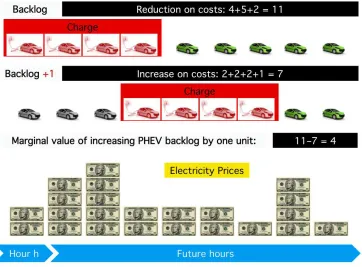
To summarize, the marginal value of increasing PHEV backlog by one unit can be
estimated by the net reduction on electricity generation costs, written as
vh+,n = L
X
l=2
CP ×P¯hn+l−1− min
h+1≤τ≤H−L+1
L
X
l=1
CP ×P¯τn+l−1. (2.35)
From (2.35) we can see that when future electricity prices are low, gains from
increasing PHEV backlog will be relatively large, meaning that more vehicles’
Fig. 2.3. Illustrating how to obtain a new sample estimate of the value function gradient approximation given the wholesale electricity price approximations
shows that using the designed value function approximation, combined with the
iter-ative updating operation, a closed feedback loop is created to make better and better
decisions.
We now use the new estimate vh+,n to update the value function gradient approx-imation according to the following equation
¯
Vh+,n= (1−α+
n−1)×V¯ +,n−1
h +α
+
n−1×v +,n
h , 2≤n≤N, 1≤h≤H; (2.36)
where α+
n−1 is a step-size between 0 and 1; and, the common practice is to use a