The impact of large lending on bank efficiency in U S A

Munich Personal RePEc Archive

The impact of large lending on bank

efficiency in U.S.A.

Andriakopoulos, Konstantinos and Kounetas, Konstantinos

Hellenic Open University, University of Patras, Department of

Economics

15 September 2019

Online at

https://mpra.ub.uni-muenchen.de/96036/

1

The impact of large lending on bank efficiency in U.S.A.

Konstantinos Andriakopoulosa and Konstantinos Kounetasb

a _{School of Social Science, Hellenic Open University, Greece}

b _{Department of Economics, University of Patras, Greece}

Abstract

This paper investigates a rather neglected issue in the banking literature regarding the impact of large lending (LL) on the three banks’ performance aspects (cost, profit and productive). Possible influences may arise in the context of banks’ credit risk as trade credit, which is provided by large, creditworthy firms, and it is a method of monitoring and enforcing loan contracts to relatively riskier firms. Indeed, trade credit providers view payments beyond the discount period as a sign of financial difficulty while the option to cut off shipments for nonpayment is a potentially powerful means for a trade creditor to force repayment, especially if a supplier provides its costumer with a product that has no close substitutes. A unique dataset was constructed concerning all USA banks collected from SDI (Statistics on Depository Institutions) report compiled by FDIC (Federal Deposit Insurance Corporation). Our sample contains 7960 banks and tracked yearly for the period 2010 -2017, creating an unbalanced panel of year observations. An econometric framework based on nested non-neutral frontiers, was developed to estimate the influence and the decomposition of large lending on the three banks' performance aspects (cost, profit and productive). Moreover, different types of frontiers aiming at the cost, profit, and production side have been investigated. The empirical findings reveal that the large lending plays a crucial role on banks' technical efficiency. Significant variations among different frontier models, type of bank and size, banks’ ownership structure and macroeconomic conditions appear to be present. By considering all CAMEL (Capital Adequacy Asset Quality Management Earnings Liquidity) parameters we notice that banks’ financial strength affects banks’ efficiency. Some policy implications are derived based on the empirical evidence supporting a safer and sounder banking system can be emerged as banks finance large firms, increasing the willingness of people to save and bank’s attitude to finance profitable investments projects that rise firm’s value and promote economic growth.

JEL classifications: C33; G21; G30

Keywords: Large lending, Τrade credit, Βank efficiency, Stochastic frontier analysis, Cost and production function

2

1.

Introduction

Trade credit remains the single largest source of short-term business credit in

the United States and other nations around the world. The tendency of production

firms to act as financial intermediaries—a role usually reserved for banks- has triggered the interest of policy makers and academics. The debate mainly focuses on

(i) explanations that view trade credit as a method of monitoring and enforcing loan

contracts to relatively risky firms, (ii) explanations in which a firm’s long-term supply relationship helps it to make better credit decisions than a bank would,(iii) the

relationship between bank credit and trade credit, and (v) the availability of credit to

small- and medium-sized enterprises from suppliers and banks. Another, equally

important topic, is the effects of large lending (LL) on bank efficiency provided that

trade credit is mainly offered by large and old firms that have access to external

finance. This paper contributes to the literature discussing this theme. We examine

whether large lending has positive or negative effects on bank efficiency. To the best

of our knowledge, this is the first paper that provides empirical evidence on this

policy relevant topic. This paper examines the impact of large lending on bank

efficiency by using stochastic frontier analysis for a broad sample of 7960 commercial

and savings banks in USA. It explores the issue by addressing four related questions:

(i) What is the effect of large lending on bank inefficiency? (ii) Large lending could

be used as an input in production function? (iii) Large lending could be used as an

output in cost function? (iv) Large lending could be used as an output in profit

function?. We will show that large lending has a positive effect on bank efficiency.

More importantly, we provide empirical evidence for the hypothesis that large lending

increases bank efficiency, the bank efficiency increasing effects of a rise in large

3

addition, we find that large lending could be used as output in cost function but not in

profit function. Particularly, banks can reduce their total cost as lending large firms

banks can avoid the cost that stem from monitoring and enforcing loan contracts to

relatively risky firm. Finally, the estimation results support that large lending could be

an input in product function which means that trade credit and bank credit can be

considered as complements implying that banks lend those firms that have received

trade credit reducing at the same time banks’ credit risk.

The rest of the paper is structured as follows. In the next section we present

the relevant literature review while in Section 3 we include the econometric

methodology which will be followed. Section 4 we present the data used and the

variables definition. Section 5 discusses the estimation results. Finally, Section 6

4

2.

Trade credit, large lending and efficiency: A brief literature

overview

The widespread use of trade credit as a source of funding in modern

economies has been highlighted by a considerable number of scholars (Elliehausen

and Wolken, 1993, Rajan and Zingales, 1995, Kohler et al, 2000, Atanasova and

Wilson, 2002, Bartholdy and Mateus, 2008, Wu et al, 2011,).

For instance, Rajan and Zingales (1995) mention that trade credit (measure it

by using account payable) reaches to 15% of total assets in 1991 for a large sample of

non-financial firms, listed US firms.

Moreover, trade credit is considered to be a very expensive means of external

finance. Smith (1987) estimates an implicit interest rate of 44% per annum for those

who do not take the discount which is 2% if costumers pay back within ten days, with

net price charged for payments within 30 days.

Also, a firm may raise capital from a multitude of sources. According to the

Financial Hierarchy doctrine, firms seek external finance when they exhaust their

internal funds which top the hierarchy as being the least costly (Myers 1984; Myers

and Majluf 1984).

Intuitively, bank loan is a cheaper source of funding compared to trade credit

however bank loan procedure relates to credit risk as borrowers promise to lenders

future uncertain payments which pay back the loan amount. Nevertheless, cash is

relatively easy to divert from its intended purpose increasing the credit risk of a bank

loan as these borrowed amounts are used to finance investments projects whose

returns will repay the loan, instead under mounting financial pressure borrowers may

use the loan for unprofitable purposes or fraud decreasing dramatically the likelihood

5

Apart from large firms, banks lend SMEs, especially, in the development

phase of their expansion, SMEs depend highly upon the banking sector to obtain

funding (Boocock and Wahab, 2001). Although, large firms and SMEs create various

positive externalities on economies and social benefit, because they make important

contributions to investment, innovation, employment, and social stability (Carter and

Jones-Evans, 2006 ; Edmiston, 2007), SMEs are thought as a group of firms for which

informational asymmetries between lenders and borrowers are more pronounced due

to their financial opacity (Berger and Udell, 1998), and therefore credit rationing is

more likely to occur (Stiglitz and Weiss, 1981. Thus, financing gaps exist in SMEs

(Cassar, 2004; Howorth 2001; Wingborg and Landström, 2000) which make not only banks unwilling to lend this kind of firms but also banks face a higher credit risk

compared to large firms when they lend this kind of firms (Cassar, 2004; Howorth,

2001; Wingborg and Landstrom, 2000).

In addition, trade credit literature suggests that firms may extend credit to

their customers for financial, operational, and commercial motives. In this section we

review the implications of financial motives on bank efficiency. Borrowing goods

instead of money permits firm to make a credible commitment not to divert the loan

for unprofitable purposes. So, trade credit is a very important source of funding for

those firms considered less creditworthy, especially when financial conditions are

difficult and financial markets are tight (Burkart and Ellingsen, 2002).

In other words, the presence of supplier - customer relationship determines

trade credit as a powerful tool that improves monitoring and enforcement since

supplier can cut off shipments for nonpayment while at the same time trade creditors

concern about the long term health of their costumers which ensures more sales in the

6

2003). Indeed, Smith (1987) shows that firms which sell products to other firms have

a screening motive to find out the default risk of their buyers.

Particularly, Smith (1987) supports that firms can manage nonsalvageables

investments effectively if they have information about buyer's default risk. Therefore,

he notices that selling firms can detect buyers' default risk offering cash discounts

payments as buyers who do not exploit this opportunity might have experienced a

deterioration in their creditworthiness. Therefore, selling firms, which offer trade

credit, have more time to take steps in order to preserve nonsalvageables investments.

In contrast to this, firms which claim net payments on cash do not have this

opportunity. So, this kind of investments influences selling firms to use trade credit as

a screening mechanism to acquire important information about buyer’s default risk. Similarly, trade credit providers view payments beyond the discount period as

a sign of financial difficulty (Ng et al, 1999 ; Petersen and Rajan, 1994) while the

option to cut off shipments for nonpayment is a potentially powerful means for a trade

creditor to force repayment, especially if a supplier provides its costumer with a

product that has no close substitutes (Berlin, 2003).

Moreover, some scholars notice that larger and older firms typically have

larger accounts receivable which means that they are large suppliers of trade credit

(Petersen and Rajan, 1997; Berlin, 2003). Firm’s age and firm’s size reflect firm’s creditworthiness a crucial characteristic that determines who is more likely to extend

trade credit as reasonably creditworthy firms have an advantage monitoring riskier

firms, which are typically smaller and younger (Petersen and Rajan, 1997; Nilsen,

2002; Berlin, 2003).

In addition, Schwartz (1974) developed the financial motives for the use of

7

increasingly offer more trade credit to maintain their relations with smaller customers,

who are "rationed" from direct credit market participation. The seller firm acts as a

financial intermediary to customers with limited access to capital markets, thus

financing their customers' growth. Faulkender and Wang (2006), also observe that

larger firms are thought to be better known and have better access to capital markets

than smaller firms, in terms of availability and cost, and should therefore face fewer

constraints when raising capital to finance their investments Hence, the financial

motive predicts a positive connection between extending trade credit and firm size

(Schwartz 1974; Petersen and Rajan 1997; Mian and Smith 1992). Consequently,

according to financial motive we establish the following hypothesis:

H1: Large lending affects positively bank efficiency

We investigate this association focusing not only on the cost efficiency, which

is the most famous dimension of bank efficiency (Silva et al 2017), but also on profit

efficiency and production efficiency two other dimensions of bank efficiency which

need more exploration as banks may be cope with cost inefficient through higher

revenue generation (Sensarma, 2005). In addition, profit function includes the same

exogenous variables with cost function (a vector of outputs and a vector of input

prices) (Sensarma, 2005).

Moreover, banks prefer to lend suppliers who extend trade credit to their

customers (Berlin, 2003), ensuring their loans as suppliers have a monitoring and

enforcing advantage over banks (Biais and Gollier, 1997). In addition, trade credit

literature considers trade credit and bank credit as complements implying that banks

lend those firms that have received trade credit (Cook, 1999; Omo, 2000; Love et al,

2007; Cunningham, 2005) as trade credit may represent a positive signal for banks

8

faces the default risk of the buyer, which means that he has good information about

the latter. Bank observes trade credit procedure and therefore it adjusts favorably its

beliefs about the buyer deciding to lend him. In other words, bank credit rationing can

be mitigated by the presence of trade credit as it permits the private information of the

seller to be used in the lending relationship, (Biais and Gollier, 1997).Therefore, we

create the below hypothesis:

H2: Large lending could be used as an input in production function

In addition, larger and older firms have easier access to external finance; they,

in turn, act as intermediaries and extend trade credit to other, riskier firms (Petersen

and Rajan, 1997). Therefore, suppliers are financial intermediaries which means that

banks can avoid the cost that stem from monitoring and enforcing loan contracts to

relatively risky firm (Berlin, 2003). Obviously, banks cannot avoid costs that are

related with efforts needed to monitoring and enforcing loans contract to large firms

which are the main source of trade credit. Thus, we test the next hypothesis:

H3: Large lending could be used as an output in cost function

Lastly, from a profit perspective, Stiglitz and Weiss, (1981) imply that banks’ profitability can be affected negatively by increased interest rate because of

information asymmetries issues that arise during bank loan procedure. Indeed, an

increase in interest rate in credit markets where lenders are not able to distinguish bad

borrowers from good borrowers, persuade low quality borrowers to apply for loans as

they face higher probabilities of default on their loans and therefore, they are harmed

less than good borrowers in case of an increase in interest rates. In other words,

lenders are keen to offer low interest rates so as to create a less risky bank loan

9

In addition, increased interest rates tend to diminish borrower’s stake in the project while at the same time under limited liability borrowers are not harmed by a

rise in interest rates when borrowers are declared insolvent. This moral hazard

justification implies that this contraction in borrowers’ profits convince them to undertake projects with high private benefits, or to abandon the initial project in favor

of alternative activities, or get involved in fraud. Thus, the likelihood of compensation

is negatively influenced by reduced performance (Stiglitz and Weiss, 1981).So, we

test the next hypothesis

H4: Large lending could be used as an output in profit function

To investigate the above hypotheses, this research employs stochastic frontier

analysis (SFA)1 _{examining the uncertain relationship between the extent of large}

leanding and the three different aspect of efficiency of USA banks. Based on Battese

and Coelli (1995), we implement the maximum likelihood estimation method to

simultaneously estimate the stochastic function and the inefficient model. Moreover,

exploring the above hypothesis we contribute to the bank efficiency literature review

which focus mainly lie in ownership structure (Bonin et al., 2005; Lensink et al.,

2008; Berger et al., 2009), mergers and acquisitions (Lee et al., 2013; Montgomery et

al., 2014) regulatory and supervisory measures on bank efficiency (Barth et al., 2010;

Chortareas et al., 2012), and corporate governance on bank efficiency (Aebi et al.,

2012; Beltratti and Stulz, 2012).

1 _{We use stochastic frontier analysis (SFA) rather than data envelopment analysis (DEA). The main}

10

3.

Methodological Issues

The most prominent and influential approach to firms’ productive performance measurement is relied on the estimation of a parametric or non-parametric production

frontier, which directly links productive efficiency notion to the notion of productive

efficiency as it was introduced, by Farell’s seminal paper (1957). The popularity of the production frontiers approach to the productive performance measurement is

mainly established on the grounds of its ability to decompose the overall productive

efficiency in components, which are mainly oriented either to the production mix

itself, either to exogenous factors which are accounted as productive inefficiency

factors. In addition, it is not worthless to mention that the approach of the parametric,

which include the so-called stochastic, production and cost frontiers, allows us to test

the hypothesis that (i) the LL function affects the kernel of the frontier and thus are

treated, in econometric terms, as an “additional input” in the production process or (ii) they are simply exogenous factors that may affect, in every possible direction, the

firms’ productive efficiency. Of course, both of the aforementioned hypotheses may not be accepted and thus no impact of LL on firm’s productive performance is identified.

3.1. LL affects the Frontier

Following Kumbhakar and Lovell (2000, p.262) let

(

x1,...,xN

)

0be an input vector used to produce scalar outputy0. The stochastic production frontier may be

written as:

11

where iindexes banks, tindexes time, ln f

(

x_it;β

)

is the deterministic kernel of the

stochastic production frontier _ln f

(

xit;β

)

+v_it_,

(

)

2

~ 0,

i v

v iid N  captures the effect

of random noise on the production process, u_i ~N

(

0,_u2

)

captures the effect of technical inefficiency and β is the parameter vector to be estimated. Hereafter the

subscript t is suppressed and fixed effects panel data models are employed for simplicity reasons. Battese and Coelli (1992) show that the best predictor of the

technical efficiency of each producer is TE_i =exp(−uˆ_i), where uˆ_i =E u

(

_i

(

v_i−u_i

)

)

. In the above described model, the so-called Error Component Model (ECM), LL may

influence the productive performance through their inclusion in the input mix. Such

being the case, LL are econometrically treated as an additional input, and the

corresponding stochastic production frontier can be written as:

lny_i =ln f

(

x_i,x_LL; ,β β_LL

)

+ −v_i u_i, i=1,...,I (2) where x_LLis the employed LL which operates as a shifter of the deterministic part of

the production frontier,β_LL is the vector of the additional parameters to be estimated

and captures the alteration of the position and shape and the production frontier due to

the inclusion of x_LL.

3.2. LL as Inefficiency Factors

In the next step we consider the case where a vector of exogenous variables

(

z1,...,zQ

)

influences the structure of the production process by which inputs x is

converted to outputy. The elements of zcapture features of the environment in

12

variables beyond the control of those who manage the production process. In this

case, as Huang and Liu (1994) proposed, the stochastic production frontier of

equation (1) is accompanied by the technical inefficiency relationship

u_i =g

(

z_i;δ

)

+_i (3) where δis a vector of parameters which are associated to inefficiency factors, to be

estimated. The requirement that u_i =_g

(

z_i;δ

)

+_i_0is met by truncating _i from

below such that_i  −g

(

z ;_i δ

)

, and by assigning a distribution to _i such

that

(

2

)

~ 0,

i N 

  . This allows _i 0 but enforces u_i 0. In the case in which the g

function is a linear one, the above model is the so-called Technical Efficiency Effects

Model (TEEM) which was introduced by Batesee and Coelli (1995). The technical

efficiency of the i−thbank is given by TE=exp

 

−u_i =exp



−δ'z_i−_i



. In this paper we test the hypothesis that the LL may have the character of a zvariable which

we name itz_LL, and thus relationship (3) becomes:

u_i =g

(

z z_i; _LL; ;δ δ_LL

)

+_i (4) where δLLare the additional parameters which have to be estimated since the LL have

been included among the other inefficiency factors. According to equation (4) LL do

not influence the structure of the production frontier, but they do influence the

technical efficiency with which banks approach the production frontier.

3.3. LL as an Input and an Inefficiency Factor

In order to test the hypothesis that LL affects the production process through

both the position and shape of the production frontier and the inefficiency term,

13

(

)

(

)

ln ln ; ;

; ; ;

i LL LL i i

i LL LL i

y f v u

u g 

= + −

= +

i ;

i

x x β β

z z δ δ (5)

The essential novelty of the Huang and Liu (1994) approach is that the

function g

(

z_i;δ

)

is allowed to include interactions between exogenous factors z_iand

production inputs xi (Batesse and Broca, 1997). The incorporation of non-neutral

effects of LL in the production performance can be realized either through the

consideration of LL as a factor that affects the production frontier itself, or through

the consideration of LL as a technical efficiency factor. In the former case, the

(

;

)

g z_i δ function for the i−thbank can be written as:

(

, , ; ,

)

ln ln

Q Q N Q

LLi LL q qi qn qi i LLq q LL

q q n q

g z x_{i ni} x δ δ _qi =



 z +



 z x +



 z x (6) The last term of the right-hand part of equation (6) depicts the non-neutral

effects of the LL on the inefficiency terms when they affect productive performance

through the kernel of the stochastic production frontier. In the case where LL are

considered an inefficiency factor exhibiting non-neutral effects, the g

(

z_i;δ

)

function for the i−thbank can be written as:

(

, , ; ,

)

ln ln

Q Q N N

LL LL q qi LL LL qn qi ni nLL LLi ni

q q n n

g z z_{i i} x_i δ δ =



 z + z +



 z x +



 z x (7)

The last term of the right-hand part of the above equation depicts the

non-neutral effects of the LL on the inefficiency terms when LL are an inefficiency factor.

The total effect of LL on the technical inefficiency of the i−thbank is the sum of the second and fourth term of the right-hand part of the above equation. Of course,

combining equations (6) and (7) we can explore the case where non-neutral effects

arise from both the LL as a factor that affects the production frontier as well as from

14

productive performance, may be based, in econometric terms, on the non-neutral

effects that our model allows for.

In the current paper the production frontier of the banks is assumed to be

described by the following translog functional form which is associated, through the

inefficiency factor v to a linear inefficiency model. That is, we consider the following

production frontier for the i th− bank with subscript t suppressed:

0

2

1

ln ln ln ln

2 1

ln 2

i n ni nm ni mi T

n n m

TT Tn ni i i

n

y x x x T

T T x u v

   

 

= + + + +

+ + + −







(8)

where n m, =L l E D LL, , , , denote , labor, liabilities, total equity, deposits, and LL

inputs respectively, while Tis a time variable which captures technical change. The

symmetry condition requiresb_nm=b_mn ,n m. As mentioned above in this paper, we

consider the case whether LL affects productive performance through their inclusion

in the input mix. In other words, the LL alters the position and the shape of the

frontier itself.

3.4. Cost and Profit Frontiers

In a similar vein we can test the hypothesis that LL affects the cost process

through both the position and shape of the cost frontier and the inefficiency term,

therefore the following model arises:

(

)

(

)

ln ln , ; ; ; ; ; ;

i LL LL i i

i LL LL i

tc f y p y v u

u g 

= + +

= +

i i

i

β β

z z δ δ (9)

Where

(

y₁,...,y_M

)

0be an output vector that requires total cost tc0given

15

the only difference that profit replaces cost as the dependent variable in the frontier

regression. Therefore, the alternative profit frontier, companying with the inefficiency

model, is given by

(

)

(

)

ln ln , ; ; ;

; ; ;

i LL LL i i

i LL LL i

f y p y v u

u g





= + +

= +

i i

i

β β

z z δ δ (10)

where π is the profit of the bank and the other variables are as explained before

In that case the function g

(

zi;δ

)

is allowed to include interactions between exogenous factors zi and outcomes yi as well as between exogenous factors zi and

input pricesp_i (Batesse and Broca, 1997). The incorporation of non-neutral effects of

LL in the cost(profit) performance can be realized either through the consideration of

LL as a factor that affects the cost(profit) frontier itself, or through the consideration

of LL as a technical efficiency factor. In the former case, the g

(

z_i;δ

)

function for the th

i− bank can be written as:

(

, , , ; ,

)

ln ln ln

Q Q M Q N Q

n m LLi LL q qi qm qi i qn qi i LLq q LL

q q m q n q

g z_i p y_{i i} y δ δ _qi =



 z +



 z y +



 z p +



 z y (11)

The last term of the right-hand part of equation (11) depicts the non-neutral

effects of the LL on the inefficiency terms when they affect cost(profit) performance

through the kernel of the stochastic cost(profit) frontier. In the case where LL are

considered an inefficiency factor exhibiting non-neutral effects, the g

(

z_i;δ

)

function for the i−thbank can be written as:

(

, , , ; ,

)

ln ln ln

Q Q N Q N M

LL n LL q qi LL LL qn qi ni qn qi i mLL LLi mi

q q n q n m

g z z_{i i} p y_{i i} δ δ =



 z + z +



 z y +



 z p +



 z y (12)

The last term of the right-hand part of the above equation depicts the

16

The total effect of LL on the technical inefficiency of the i−thbank is the sum of the second and fourth term of the right-hand part of the above equation. Of course,

combining equations (11) and (12) we can explore the case where non-neutral effects

arise from both the LL as a factor that affects the total cost frontier as well as from LL

as an inefficiency factor. Thus, the multifaceted character of LL, as regards cost and

profit performance, may be based, in econometric terms, on the non-neutral effects

that our model allows for.

Most studies on the determinants of banks’ technical efficiency use data envelopment analysis (DEA) or stochastic frontier analysis (SFA). We use stochastic frontier

analysis as it controls for measurement error and other random effects2 We use

Battese and Coelli(1995) SFA model henceforth the BC model. that provides

estimates of efficiency in a single step in which firm effects are directly influenced by

a number of variables. A first advantage of the BC model over the standard two-step

SFA approach of Aigner et al. (1977), and Meeusen and van den Broeck (1977) is

that the former estimates the cost frontier and the coefficients of the efficiency

variables simultaneously3. Wang and Schmidt (2002) show that a two-step approach

suffers from the assumption that the efficiency term is independent and identically

half-normally distributed in the first step, while in the second step the efficiency terms

are assumed to be normally distributed and dependent on the explanatory variables.

This method inherently renders biased coefficients. A second advantage of the BC

model is that it can be estimated for an unbalanced panel, which increases the amount

2 _{Non-parametric techniques do not allow for measurement error and luck factors.}

These techniques attribute any deviation from the best practice bank to technical inefficiency. For a more extensive review of the non-parametric and the parametric approach, see Matousek and Taci (2004).

17

of observations. This study specifies the following stochastic translog cost function

with three inputs and three outputs:

2

0

2

1 1 1

ln ln ln ln ln ln ln ln ln

2 2 2

1

ln ln

2

n n

i m mi n ni mm mi mi p ni ni mp mi ni T

m n m m n n m n

tm mi tn ni i i t

m n

tc y p y y p p y p T

T T y T p u v

      

  

= + + + + + +

+ + + + +















(13)

where m= L,I,NI, and LL denote loans, investments, nοn-interest income and large lending respectively while n=L, C and F denote price of labor, price of capital and

price of funding respectively, tc represents the total cost of the i-th bank with

subscript t suppressed, _m , _n, _mm,

n

p  ,

n

mp

 , _T, _t2, tm, tn are the parameters

to be estimated. Cost and input prices are normalized by the price of labor before

taking logarithms to impose linear input price homogeneity. This scaling implies an

estimation of coefficients for pC(price of capital) as well as pF(price of funding)

with the restriction that the sum of these coefficients is equal to one (see Kuenzle,

2005).The alternative profit function uses essentially the same specification as the

cost function, but with one change. The dependent variable for the profit function

replaces the logarithm of normalized total cost with ln

 

 , compared to the cost

function, this the only change in specification, since the independent variables are

identical to those in the cost function. The inefficiency term, of course, enters the

frontier with a negative sign since now higher inefficiency is associated with lower

profits as compared with best bank. As in the cost study, profit and input prices are

normalized by the price of labor before taking logarithms to impose linear input price

homogeneity.

18

In order to provide a better illustration of our methodology, we devised figures

1,2, and 3, with four vertical flowcharts. Each of the first three charts depicts each of

the three hypotheses regarding the impact of large lending may bear on the three

banks’ performance aspect (cost, profit and productive). More specifically: (i) it affects the deterministic part of the frontier, that is, the large lending operates as an

“additional input” for the case of productive performance while it operates as “additional output” for the case of cost and profit performance; (ii) through the inefficiency term or in other words it has the character of an inefficiency factor; (iii)

both ways. The final chart depicts the hypothesis that large lending has no effects. The

full set of models that arise from these four distinct hypotheses for the case of cost,

profit and productive performance is presented in the Fig 1,2, and 3 of the paper

respectively.

To elaborate further, if we consider that large lending is an input (output for

the case of cost and profit performance), the first vertical flow chart in figures 1,2 and

3 denote that this may be approximated by an ECM specification (see model B) or

under a TEEM specification. The TEEM specification may be modeled with neutral

(see model D) or with non-neutral (see model G) effects of inefficiency terms. The

second from the left vertical flow chart indicates that large lending acts as an

inefficiency factor that can be approached by a TEEM model specification with

neutral (see model E) or non-neutral (see model F) effects of inefficiency terms.

Accordingly, the third vertical flow chart reveals that the impact of the adoption can

be approximated by only a TEEM model with neutral (see model H) or non-neutral

(see model I) effects of inefficiency terms. Finally, the last vertical flow chart assumes

19

(see model A) specification and the two versions of the TEEM (see models C and J)

specification are the ones that should be estimated4.

As we can observe from the formulation of our models, they are nested and

their differences are in the number of restrictions employed in their estimation. Thus,

we can use the generalized likelihood ratio to decide which identification is the most

appropriate and thus to reveal the role of large lending on banks’ cost, profit and productive efficiency.

[Insert Figure 1 here]

[Insert Figure 2 here]

[Insert Figure 3 here]

4 _{In the context of the non-neutral TEEM modeling procedure, two alternatives arise. The}

first alternative is the one which incorporates the non-neutral effects which are generated by the interaction of all the inputs (outputs in case of cost efficiency or profit efficiency) with all the inefficiency factors. The second alternative is the one which is restricted to the inclusion in the inefficiency model only of those terms which are generated by the interaction of only a subset of inputs (outputs in case of cost efficiency or profit efficiency) with the inefficiency factors. In the context of the present paper we have followed the second approach since the full version of the non-neutral TEEM approach incorporates thirty-two inefficiency factors and serious multicollinearity problems arise. Specifically, in all the cases where the modeling procedure considers LL an additional factor, the inefficiency model encompasses the non-neutral-effects of the x_Einput (outputs in case of cost efficiency or profit efficiency) with all the inefficiency factors.

20

4.

Data and Variables Definition

The financial and accounting data used in this study were obtained from SDI

(Statistics on Depository Institutions) report made by FDIC (Federal Deposit

Insurance Corporation). This report provides banks’ financial statements, ratios, types, ownership structure and information for USA banks. Therefore, it is the reference

database for USA samples that both offers data on large and small business loans. In

addition, SDI report is interested in what each bank considers a small business, so we

can understand the full range of small business lending activity financed by banks.

Rather than providing a definition, SDI report instead is asking each bank for its

description of what it considers a small business. In this way, we will get a better

sense of the differences in small business lending by different types of banks. Our

sample contains 7960 banks and tracked quarterly for the period 2010 -2017, creating

an unbalanced panel of bank year observations. We adopt an intermediation approach

(Berger and Humphrey, 1991; Ellinger and Neff, 1993; Altumbas et al., 2000;

Rezvanian and Mehdian, 2002) to define the factor input and output of banks.

For our estimations, we have three dependent variables, bank’s total output

( )y , is the sum of loans, investments and non-interest income ,bank’s total cost ( )tc is the sum of labor cost, capital cost and funding cost while bank’s profit (π) is the pre-tax operating income. We specify as inputs, the salaries and employee benefits(x_L),

the liabilities ( )x_l , the total equity capital(x_E), and deposits (x_D)of banks. Moreover,

We specify as outputs, the total loans (yL), the investments (yI), and the

non-interest income (y_N)of banks. In addition, we include in translog cost function,the

21

price of labor (pL)calculated as the ratio of employ salary to total employees and the

price of funding(p_F)determined as the ratio of interest payments to total liabilities. In

the cases where the impact of LL on the deterministic part of the frontier is tested, and

thus the LL is regarded as an additional input, the values of x_LL are derived from the

difference between commercial and industrial loans minus commercial and industrial

lending to small business divided by loans and lease financing receivables of the

institution, including unearned income.

The variables which are incorporated in the inefficiency model may be

grouped in two categories. The first category encompasses variables which are

determined by the CAMEL model and therefore they depict the financial health of the

bank and consequently its overall economic strength. Beginning with the first

acronym of CAMEL model we have constructed the variable (CAP), that represents bank’s capital adequacy and it is defined as the ratio of the sum of Tier 1 (core) capital plus Tier 2 Risk-based capital divided by bank’s total assets. Also, we have used variables that reflects bank’s asset quality such as (NPLS3), which is defined as the ratio of total assets past due 30 through 89 days and still accruing

interest to the bank's total assets as well as the variable (NPLS3), defined as the

ratio of total assets past due 90 or more days and still accruing interest to the bank’s total assets. Moreover, we have created the management capability variable (MAN),

defined as the ratio of net operating income to total not interest expenses. In addition,

the variable (ROA), net income after taxes and extraordinary items (annualized) as a

percent of average total assets, reflects banks’ profitability while the last acronym of the CAMEL model includes the variable (LIQ)that represents banks’ liquidity and it

22

including unearned income to total deposits. The second group of the inefficiency

factors contains county-specific factors that expected to influence banks’ efficiency. In this category we have included the Herfindahl index variable(HHI), as a proxy

for the structural market conditions that entails in each county. Ιn the same category of the inefficiency factors we have included the industry specific dummy variables

(COM), and(SAV). Especially,(COM), variable takes the value of 1 for

commercial banks and 0 for savings banks. Similarly, (SAV), variable takes the value

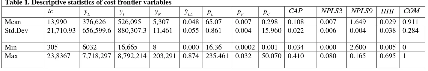
of 1 for savings banks and 0 for commercial banks. Table 1,2 and 3 provide

descriptive statistics for all variables used in the estimation of the cost, profit and

production frontier and the inefficiency model respectively.

[Insert Table 1 here]

[Insert Table 2 here]

23

5.

Results and discussion

5.1. Characteristics of the frontier and the inefficiency model

All the models which are analytically presented in figures 1,2 and 3 have been

estimated using Frontier 4.1 software (Coelli, 1996). It should be noted, that in all the

estimated models the relevant tests indicate that the null hypothesis of no technical

inefficiency effects

(

 =0

)

in the estimated production frontier is not accepted5.In

addition, a range of specification tests was carried out for all the estimated frontiers

aspects (cost, profit and production) including a test for the specification of the three

frontiers aspects (cost, profit and production) as Cobb-Douglas (CRS).In all the cases

the hypotheses that the functional form of three frontier aspects(cost, profit and

production) is of the Cobb-Douglas type and that the technology exhibits Constant

Returns to Scale were not accepted.

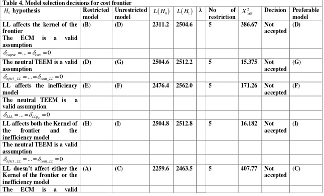
Models D, F and C are nested to Model I΄, and simple likelihood ratio tests indicate that the last is superior in econometric terms in case of banks’ cost performance (Table 4). Thus, it can be argued that LL affects the banks' cost

performance both through the position and shape of the frontier and the inefficiency

term. Thus, and hereafter the discussion will be focused on the estimation results of

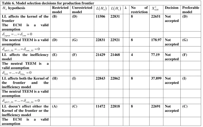
Model I΄. Similarly, the same analysis conducted in the case of banks’ profit and productive performance (Table 5 and Table 6 respectively) concluding that Model I΄ is greater in econometrics terms and therefore the conversation will be focused on the

estimation results of Model I΄.

[Insert Table 4 here]

5 _{This test is carried out in the form of the likelihood ratio test. The critical value for testing}

24

[Insert Table 5 here]

[Insert Table 6 here]

5.2 Cost Efficiency Results

The estimates of the inefficiency model are summarized in the lower part of

Table 7. The null hypothesis that the coefficients of the inefficiency factors are jointly

zero is not accepted. Surprisingly, technical efficiency is negatively affected by the

banks’ financial strength as it is captured by the variable of capital adequacy. This result does not confirm the argument that higher capitalization contributes to alleviate

agency problems between managers and shareholders. Shareholders in this case have

greater incentives to monitor managements performance and ensure that the banks are

run efficiently (Eisenbeis et al., 1999).

Similarly, non-performing loans past due 90 days or more affects negatively

technical inefficiency contrary to financial theory that supports that non-value-added

activities of bad assets incur a negative consequence on the operating performance

(Tsai and Huang, 1999). In addition, market construction seems to influence

negatively banks’ technical inefficiency confirming the Efficient Structure Hypothesis, that most efficient banks are likely to survive competitive pressures and

they will gain market share at the cost of less efficient banks (Demsetz, 1973).

Finally, commercial banks firms are revealed to be more efficient compared to

savings banks.

5.3. The Impact of large lending on Cost Efficiency

25

impact of large lending on banks’ total cost performance is traced in both the deterministic kernel of the stochastic frontier and the inefficiency model.

Concerning the deterministic part of the model, it is evident that large lending

influence the total cost since both the coefficient of the

( )

y_LL variable and the

coefficient of the

( )

y_LL 2variable is negative. In addition, large lending affects negatively total cost when it interacts with non-interest income output and time trend

variable which captures the technological change while it affects positively the total

cost when it interacts with investments variable. The interaction of large lending with

price of capital reveal a negative relationship between total cost and price of capital.

Contrary, we notice a positive relationship between total cost and price of funding

when large lending interacts with the price of funding. Apparently, a non-monotonic

performing between the large lending and the banks’ cost performance is in place. Further elaboration of this relationship is presented below in this section.

Turning to the inefficiency model, large lending reduces technical

inefficiency when no non-neutral effects are taken into account. When the latter

appear, we can identify the positive influence of large lending on the firms’ technical efficiency, when they are combined with the price of capital variable and the variable

that represent bank’s investments and banks’ non-interest income. In contrast, the interaction of the large lending with the price of funding reveals a negative influence

on the banks’ technical efficiency is rather expected.

Finally, the interaction of large lending with non-performing loans past due 90

or more days reveals the unexpected negative relationship between banks’ inefficiency and non-performing loans.

26

5.4. Profit Efficiency Results

As discussed earlier, it is important to look at the revenue side of bank

operations. Accordingly, the estimates of profit efficiency are presented in Table 8.

As in the cost case, we focus on model I΄. The null hypothesis that the coefficients of the inefficiency factors are jointly zero is not accepted. Τhe empirical results summarized in the lower part of Table 8 suggest that technical efficiency is positively

affected by the bank’s financial strength as it is captured by the non-performing loans variables. We find that non-performing loans have a positive relationship with banks

profit inefficiency supporting the related literature that suggests that efficient banks

are better at managing their credit risk (Berger and DeYoung, 1997).

Moreover, capital ratio influences negatively profit inefficiency implying that

higher capital ratios are related with greater efficiency consisting with the argument

that higher capitalization contributes to alleviate agency problems between managers

and shareholders. Shareholders in this case have greater incentives to monitor

managements performance and ensure that the banks are run efficiently (Eisenbeis et

al., 1999). Finally, commercial banks firms are revealed to be more efficient

compared to savings banks.

5.5. The Impact of large lending on Profit Efficiency

Starting with the kernel of the stochastic frontier we notice that large lending

influence positively banks’ profits when interacts with investments output and time trend variable which captures technological change while this relationship turns to

negative when large lending interacts with total loans output. Moreover, the

interaction of large lending with price of funding and price of capital do not reveal

27

monotonic. Additional amplification of this association is presented below in this

section.

As far as the inefficiency model, large lending reduces technical inefficiency

when no non-neutral effects are taken into account. When the latter appear, we can

identify the positive influence of large lending on the firms’ technical efficiency, when they are combined with total loans output and banks’ investments output. However, the interaction of the large lending with the price of capital and the price of

funding seems to not alter the negative relationship between technical inefficiency and

large lending. Similarly, the above relationship does not change when large lending

interacts with non -interest income output.

Moreover, we can identify the positive influence of large lending on the

banks’ technical inefficiency, when they are combined with the non-performing loans past due 90 days variable. Thus, we can argue that an poor asset quality are in general

technical inefficiency increasing, as we have already seen above, in the case of large

lending non-performing loans past due 90 days seems to not be affected by the ability

of large lending to decrease banks credit risk alleviating the information asymmetry

problems that arise during a loan procedure. In contrast, the interaction of large

lending with market structure confirms the Efficient Structure Hypothesis that implies

a negative relationship between banks’ inefficiency and market power while the interaction of large lending with industry specific variable show the expected negative

association between commercial bank and banks’ inefficiency since this dummy capture banking technology that contains less credit risk.

[Insert Table 8 here]

28

Based on model I΄ we explore banks technical efficiency in terms of product performance. The estimates of the inefficiency model summarized in Τable 9. The null hypothesis that the coefficients of the inefficiency factors are jointly zero is not

accepted. Technical efficiency is positively affected by the bank’s financial strength as it captured by the variables of CAMEL model. Particularly, we find that

non-performing loans have a negative relationship with banks efficiency confirming that a

large proportion of non-performing loans may signal that banks use fewer resources

than usual in their credit evaluation and loans monitoring process (Karim et al 2010).

Similarly, capital ratio influences negatively technical inefficiency implying that

higher capital ratios are related with greater efficiency consisting with the argument

that higher capitalization contributes to alleviate agency problems between managers

and shareholders (Eisenbeis et al., 1999). In a similar vein, the cost to income ratio

influence positively product inefficiency suggesting that a poorer management’s ability to control costs reduces cost inefficiency as higher expenses normally mean

higher cost and vice versa.

Surprisingly, the liquidity ratio affects negatively the cost inefficiency

indicating that banks inefficiency reduces as liquidity risk increases. As Golin (2001)

In addition, market construction seems to influence positively banks’ technical inefficiency confirming the “quiet-life” effect, postulating that the greater the market power, the lower the effort of managers to maximize operating efficiency. (Berger and

Hannan, 1998). Finally, commercial banks firms are revealed to be more efficient

compared to savings banks.

5.7. The Impact of large lending on Product Efficiency

Concerning the kernel of the stochastic frontier, it is evident that large lending

29

negative supporting the substitution hypothesis between bank credit and trade credit.

In addition, large lending affects negatively the produced output when it interacts with

liabilities input and total equity input while it affects positively the produced output

when it interacts with labor input. Apparently, a non-monotonic performing between

the large lending and the banks’ product performance is in place. Further elaboration of this relationship is presented below in this section.

Regarding the inefficiency model, we notice that large lending reduces

technical inefficiency when no non-neutral effects are taken into account. When the

latter appear, we can identify the positive influence of large lending on the firms’ technical efficiency, when they are combined with labor input and total deposits input.

In contrast, the interaction of the large lending with banks’ liabilities input and total equity of capital input seems to not alter the negative relationship between

technical inefficiency and large lending.

In addition, we can identify the positive influence of large lending on the

banks’ technical inefficiency, when large lending is combined with the non-performing loan variable. Thus, we can argue that an poor asset quality in general are

technical inefficiency increasing, as we have already seen above, in the case of the

large lending non-performing loans increase banks’ inefficiency as a large proportion of non-performing loans may signal that banks use fewer resources than usual in their

credit evaluation and loans monitoring process (Karim et al 2010). Similarly, the

interaction of large lending with market structure confirms the “quiet-life” effect (Berger and Hannan, 1998). In addition, this relationship seems to alter when large

lending interacts with capital adequacy variable implying that although banks use

trade credit to reduce information asymmetry problems however it still contains credit

30

Finally, the interaction of large lending with industry specific variable show

the expected negative association between commercial bank and banks’ inefficiency since this dummy capture banking technology that contains less credit risk.

31

6.

Conclusions

Large firms (opaque firms) is particularly important for banks since an

important part of lending to these kinds of firms is transported to trade credit provided

to financially constrained firms (smaller and less liquid firms). Consequently, large

lending could improve banks’ technical efficiency significantly. Though the impact of large lending on banks’ technical efficiency is highly important, no studies have been carried out to examine this relation. The objective of this article is to provide

empirical evidence of the effect of large lending on the banks’ technical efficiency for the three efficiency aspects (product, cost and profit) using a sample of USA banks

during the period 2010-2017. We find a positive relationship between the investment

in large lending and banks’ technical efficiency for all measures derived from the fact that the benefits associated to trade credit surpass the costs of banks’ credit risk. Further evidence supports the complements relationship between bank credit and

trade credit, showing large lending enters positively and significantly in production

function implying that banks provide credit to those firms that have been granted trade

credit by suppliers. The findings also support the financial motive for trade credit.

Actually, the use of large lending as output in cost function can decrease banks’ cost. In this sense, large lending might be used to alleviate banks’ credit risk, thus lowering operating costs and therefore enhancing bank profitability. However, we do not find

evidence for the financial motive, when we focus on profit function as large lending

does not enter significantly in our regression.

These results show the important role of large lending as a determinant of

banks’ technical efficiency and provide valuable insights for academics and bankers since the results suggest that by increasing their investment in large lending

32

of current assets management in the maximization of bank value and opens an

important field for future research. However, this study is also relevant for other

groups of stakeholders, such as central banks and policy makers since central banks

play a key role in the monitor the banking system and policy makers, in view of the

importance of large lending for banks’ technical efficiency, should enforce loan contracts to combat late payment in large lending.

To finish, one possible limitation is that the study focuses on a period of

economic recovery (2010-2017) for the USA banking system. From our point of view,

the over-time robustness of the findings is interesting. It would be appropriate to

replicate this study in a period of economic downturn, like the 2007 financial crises,

when data are available, in order to compare the results and draw conclusions. Due to

liquidity and financial constraints arising from the current financial crisis, the

relations obtained could be different. Late payment or non- payment in commercial

transactions has increased significantly and because of this the positive relation found

between the investment in large lending, given that large lending transported to trade

33

Tables

Table 1. Descriptive statistics of cost frontier variables

tc y_L y_I y_N y_LL p_L p_F p_C CAP NPLS3 NPLS9 HHI COM

Mean 13,990 376,626 526,095 5,307 0.048 65.07 0.007 0.298 0.108 0.007 1.649 0.029 0.911 Std.Dev 21,710.93 656,599.6 880,307.3 11,461 0.055 0.861 0.004 15.960 0.022 0.006 0.004 0.038 0.284

Min 305 6032 16,665 8 0.000 16.36 0.0002 0.001 0.034 0.000 2.600 0.005 0

[image:34.842.64.778.126.245.2]

Max 23,8367 7,718,297 8,792,214 203,291 0.874 235.461 0.032 50.070 0.410 0.080 0.165 0.695 1

Table 2. Descriptive statistics of profit frontier variables

 y_L y_I y_N y_LL p_L p_F p_C CAP NPLS3 NPLS9 HHI COM

Mean 7,047.533 384,409.2 540,272 5,567.803 0.049 65.4655 0.006 0.303 0.107 0.006 0.001 0.031 0.915

Std.Dev 13,967.47 688,564.4 920,396.4 12,499.04 0.057 16.065 0.004 0.817 0.025 0.006 0.004 0.041 0.278

Min 2 6,516 13,820 8 7.064 16.362 0.0002 0.001 0.023 5.035 2.594 0.005 0

[image:35.842.61.824.95.226.2]

34

Table 3. Descriptive statistics of product frontier variables

y

L

x xl xN xLL CAP NPLS3 NPLS9 MANAG ROA LIQ HHI COM

Mean 892,409 504,004.3 61,188.64 135643.3 0.049 0.107 0.006 0.001 7.337 0.996 0.761 0.030 0.914

Std.Dev 1,524,122 848,903.4 111,714.7 193,670.1 0.056 0.025 0.006 0.004 67.093 0.509 0.180 0.040 0.279

Min 22,736 14,590 1,625 1,013 7.064 0.023 5.035 2.594 0.292 0.002 0.060 0.005 0

[image:36.842.95.741.119.511.2]

35

Table 4. Model selection decisions for cost frontier

0

H hypothesis Restricted

model

Unrestricted

model

( )

0

L H L H

( )

1 λ No of

restriction 2 0.05

X Decision Preferable

model LL affects the kernel of the

frontier

The ECM is a valid

assumption

(B) (D) 2311.2 2504.6 5 386.67 Not

accepted (D)

... 0

caprat com  = = =

The neutral TEEM is a valid assumption

(D) (G) 2504.6 2512.2 5 15.375 Not

accepted (G)

3_ ... _ 0

npls LL com LL

 = = =

LL affects the inefficiency model

(E) (F) 2476.4 2562.0 5 171.26 Not

accepted (F)

The neutral TEEM is a valid assumption

... 0

F

LLL LLp

 = = =

LL affects both the Kernel of

the frontier and the

inefficiency model

(H) (I) 2504.8 2512.8 5 16.182 Not

accepted (I)

The neutral TEEM is a valid assumption

3_ ... _ 0

npls LL com LL

 = = =

LL doesn’t affect either the

Kernel of the frontier or the inefficiency model

(A) (C) 2259.6 2463.5 5 407.77 Not

accepted (C)

36

assumption

... 0

caprat com  = = =

The neutral TEEM is a valid assumption

( C) (J) 2463.5 4346.2 11 3765.4 Not

accepted (J)

3_ ... _ 0

npls LL com LL

 = = =

Horizontal decisions (D) (I) 2504.6 2512.8 6 16.605 Not

accepted (I)

3_ ... _ 0

LL npls LL com LL

 = = = =

3_ ... _ 0

LL npls LL com LL

 = = = = (C) (I) 2463.5 2512.8 14 98.658 Not

accepted (I)

3_ ... _ 0

npls LL com LL

 = = = (F) (I΄) 4562.1 2624.1 11 3875.5 Not

accepted (I΄)

... 0

F

LLL LLp

 = = = (I) (I΄) 2512.8 2624.4 5 223.12 Not

[image:38.842.98.775.89.493.2]

37

Table 5. Model selection decisions for profit frontier

0

H hypothesis Restricted

model

Unrestricted

model

( )

0

L H L H

( )

₁ λ No of

restriction 2 0.05

X Decision Preferable

model LL affects the kernel of the

frontier

The ECM is a valid

assumption

(B) (D) No

value

-9300.3 5 5 No

value

Not accepted

(D)

... 0

caprat com  = = =

The neutral TEEM is a valid assumption

(D) (G) -9300.3 -9291.8 5 16.953 Not

accepted (G)

3_ ... _ 0

npls LL com LL

 = = =

LL affects the inefficiency model

(E) (F) -9314.0 -9252.5 5 112.94 Not

accepted (F)

The neutral TEEM is a valid assumption

... 0

F

LLL LLp

 = = =

LL affects both the Kernel of

the frontier and the

inefficiency model

(H) (I) -9298.3 -9291.2 5 14.07 Not

accepted (I)

The neutral TEEM is a valid assumption

3_ ... _ 0

npls LL com LL

 = = =

LL doesn’t affect either the

K