http://www.scirp.org/journal/ojbm ISSN Online: 2329-3292
ISSN Print: 2329-3284
DOI: 10.4236/ojbm.2018.61001 Nov. 21, 2017 1 Open Journal of Business and Management
Machine Learning Methods of Bankruptcy
Prediction Using Accounting Ratios
Yachao Li, Yufa Wang
Henan Polytechnic University, Jiaozuo, Henan
Abstract
The aim of bankruptcy prediction is to help the enterprise stakeholders to get the comprehensive information of the enterprise. Much bankruptcy predic-tion has relied on statistical models and got low predicpredic-tion accuracy. Howev-er, with the advent of the AI (Artificial Intelligence), machine learning me-thods have been extensively used in many industries (e.g., medical, archaeo-logical and so on). In this paper we compare the statistical method and ma-chine learning method to predict bankruptcy with utilizing China listed com-panies. Firstly, we use statistical method to choose the most appropriate indi-cators. Different indicators may have different characteristics and not all in-dicators can be analyzed. After the data filtering, the inin-dicators are more per-suasive. Secondly, unlike previous research methods, we use the same sample set to conduct our experiment. The final result can prove the effectiveness of the machine learning method. Thirdly, the accuracy of our experiment is higher than existing studies with 95.9%.
Keywords
Bankruptcy Prediction, Statistical Method, Machine Learning, Accounting Ratios
1. Introduction
For a long time, corporate bankruptcy prediction is one of the utmost signific-ance parts in evaluating the corporate prospects. Lenders, investors, govern-ments and all kinds of stakeholders are eager to seek an efficient way to under-stand the ability of the company so that they can choose the suitable decision making. The whole condition of the corporate either small or large needs to de-velop the models to assess the financial risks. For example, Altman (1968), in a paper, used the multivariate discriminant analysis to predict the financial case
How to cite this paper: Li, Y.C. and Wang, Y.F. (2018) Machine Learning Methods of Bankruptcy Prediction Using Accounting Ratios. Open Journal of Business and Man-agement, 6, 1-20.
https://doi.org/10.4236/ojbm.2018.61001
Received: October 24, 2017 Accepted: November 18, 2017 Published: November 21, 2017
Copyright © 2018 by authors and Scientific Research Publishing Inc. This work is licensed under the Creative Commons Attribution International License (CC BY 4.0).
http://creativecommons.org/licenses/by/4.0/
DOI: 10.4236/ojbm.2018.61001 2 Open Journal of Business and Management
[1].
The original study in bankruptcy prediction can be dated back to the early 20th century when Fitzpatrick (1932) used economic index to describe predictive capacity of default business [2]. After that, more and more researchers focused on the bankruptcy prediction (e.g. Winakor and Smith(1935) [3]; Merwin,
(1942) [4]). The turning point in the survey of the business failure symptoms was happened in 1966 by Beaver who initiated the statistical models to made fi-nancial forecasts. Following the line of thinking, there are many representative statistical models were proposed by scholars [5]. Ohlson (1980) used the logistic regression to forecast financial status [6]. Besides, in 1985, West determined fi-nancial forecasts with factor analysis [7]. Similar to the experiments, a great number of generalized liner models that can be used to predict financial condi-tions emerged continuously (e.g. Aziz, Emanuel and Lawson (1988) [8]; Koh (2010) [9]; Platt, Platt and Pederson (1994) [10]; Upneja and Dalbor (2000) [11]; Beaver, McNichols and Rhie(2005) [12]et al.).
From the beginning of the 20th century, AI and machine learning methods are becoming more popular in many different industries. For example, Subasai and Ismail Gursoy (2010) [13] and de Menezes, Liska, Cirillo, and Vivanco (2016) [14] in medicine; Maione et al. (2016) [15] and Cano et al. (2016) [16] in chemistry; Heo and Yang (2014) [17] in finance; Kim, Kang, and Kim (2015)
[18] in finance. Except for those industries, it is widely used in a variety of dis-cipline. Bankruptcy prediction is one of them. With the advent of the big data era, statistical models have some weaknesses in reflect bankruptcy prediction. Based on that, researchers have to find some new method to overcome the shortcoming of statistical method. Since the bankruptcy prediction is similar to the classify algorithm, academics are exploring machine learning tools can be used to separate bankruptcy and non-bankruptcy corporate (Wilson and Sharda (1994) [19]; Tsai (2008) [20]; Chen et al. (2011) [21]). Besides, many researchers combine statistical methods and machine learning methods to enhance the real-ity of bankruptcy prediction continually. Cho et al. (2010) introduced the hybrid model by selecting variables filtered by decision tree and case-based reasoning using the Mahalanobis distance with weights [22]. Chen et al. (2009) introduced a hybrid model by combining the fuzzy logic and neural network [23]. The final results show that the hybrid model has a higher accuracy than logic model. All in all, with the development of information science, it has great influence on all fields of scientific research.
As a hot research topic in computer science, machine learning has many dif-ferent components, which consists of the decision tree, support vector ma-chines(SVM), K-nearest neighbor method (KNN), random forest, logistic re-gression , artificial neural network (ANN) and so on.
DOI: 10.4236/ojbm.2018.61001 3 Open Journal of Business and Management
this, there are many scholars using support vector machines (SVM) to recognize bankruptcy and non-bankruptcy as well (Shin et al. (2005) [25]; Chaudhuri and De (2011) [26]; Sun and Li (2012) [27]). In order to improve the accuracy of bankruptcy prediction, many scholars try to change the algorithm. Chaudhuri and De (2011) choose fuzzy support vector machine to (FSVM) to solve the problem of bankruptcy prediction and they claimed the efficient of FSVM [26]. Zhou et al. (2009) proposed a direct method to optimize parameters in SVM
[28].
Artificial neural network (ANN) establishes an analogy with neural network. The model is a structure similar to the neural network. The input layer is the input variable and the output layer determines the output variables. Between the first layer and the final layer are hidden layers. Compared with the traditional statistical models, many non-linear relationships can be analyzed by using artifi-cial neural network (ANN). Tsai (2014) introduced some machine learning me-thod to predict bankruptcy and the final result show that the accuracy is 86%
[29]. In a word, the artificial neural network (ANN) can improve the accuracy modify by setting the parameters. Based on that, the paper compares statistical methods and computer science methods to find the most effective bankruptcy prediction model.
The rest of papers proceed as follows. In Section 2, we briefly introduce the data filter processing methods and machine learning methods. In Section 3, we present the data filtering process. In Section 4, we do the experiment and display experiments result. Concluding the article and suggestions for the future re-search will be given in the last part of Section 5.
2. Methodology
2.1. Normal Distribution Test
Normal distribution is one of the components of hypothesis testing. The formula for one-dimension normal distribution is:
( )
(
2)
21 exp
2 2
x
f x µ
σ πσ
−
= −
where µ is the mean or expectation of the distribution (and also its median and mode). σ is the standard deviation. σ2 is the variance.
According to the sample size, there are usually divide into two different cate-gories:
1) If the number of samples is less than 2000, we will choose the shapiro-wilk test’s W-statistic to verify the normal distribution.
2) If the number of samples is more than 2000, we will choose the Kolmogo-rov-Smirnov test to verify the normal distribution. In this paper, our sample is less than 2000, so we are mainly to focus on the Shapiro-Wilk test.
nor-DOI: 10.4236/ojbm.2018.61001 4 Open Journal of Business and Management
mally distributed population. The test statistic is:
2 n 2 n i i i n i i n a x W x x = −
∑
∑
= =where xi is the i-th order statistic, x=
(
x1+x2+ + xn−1+xn)
n is thesam-ple mean, the constants ai are given by
(
)
(
)
T 1
1, , n T 1 1 T 1/ 2
m V
a a
m V V m −
− −
⋅⋅⋅ =
where
(
)
T 1, , nm= m ⋅⋅⋅m and m1,⋅⋅⋅,mn are the expected values of the order
statistics of independent and identically distributed random variables sampled from the standard normal distribution, and V is the covariance matrix of those
order statistics.
2.2. Wilcoxon Rank-Sum Test
Wilcoxon rank-sum test is a non-parametric test. It does not require the as-sumption of normal distributions, so it is widely used in non-parametric test. It is as effective as the t-test in parametric test on parametric test. The basic idea for Wilcoxon rank-sum test was: if the test hypothesis was established, the rank and difference of the two groups were smaller. The Wilcoxon rank-sum test steps consist of the following three steps:
1) Establish hypothesis
H0: The overall distribution of the two groups was the same;
H1: The overall distribution of the two groups is different; the inspection level was 0.05.
Create two separate samples
The first x sample size is n1, the second y sample size is n2. In the
ca-pacity of the mixed sample n= +n1 n2 (first and second), the x sample
rank-sum is Wx and the y sample ranksum is Wy.The value of Z is:
(
)
(
)
(
)
(
)(
)
( )
1 1 23 1
1 2 1 2 2
1 2 1 2
1 0.5
0.5 2
~ 0,1
1
12 12 1
x x
j j
n n n
W W
z N
n n
n n n n
n n n n
µ
σ τ τ
+ + − ± − ± = = − + + − + + −
∑
or(
)
(
)
(
)
(
)(
)
( )
1 1 23 1 1 2 1 2 2
1 2 1 2
1 0.5
0.5 2
~ 0,1
1
12 12 1
y y
j j
n n n
W W
z N
n n
n n n n
n n n n
µ
σ τ τ
+ + − ± − ± = = − + + − + + −
∑
where jDOI: 10.4236/ojbm.2018.61001 5 Open Journal of Business and Management
0.5
± is to modify the discrete variables.
According to the significance level, determine whether to accept the original hypothesis.
2.3. Principle Component Analysis (PCA)
Suppose that we have a random vector X:
1 2 p X X X X =
With population variance-covariance matrix:
( )
2
1 12 1 2
21 2 2
2 1 2
var
p
p
p p p
X
σ σ σ
σ σ σ
σ σ σ
= =
∑
Consider the linear combinations:
1 11 1 12 2 1 2 21 1 22 2 2
1 1 2 2
p p
p p
p p p pp p
Y e X e X e X
Y e X e X e X
Y e X e X e X
= + + + = + + + = + + +
Each of these can be thought of as a linear regression, predicting Yi from
1, 2, , P
X X X . There is no intercept, but e ei1, i2,,eip can be viewed as
re-gression coefficients.
Note that Yi is a function of our random data, and so is also random.
There-fore it has a population variance.
( )
1 1var
p p
i ik il kl i i k l
Y e e e e e
− −
′
=
∑∑
=∑
Moreover, Yi and Yj will have a population covariance
(
)
1 1
cov ,
p p
i j ik il kl i i k l
Y Y e e e e e
− −
′
=
∑∑
=∑
Here the coefficients eij are collected into the vector
1 2 i i i ip e e e e =
2.4.
K
Nearest Neighbors (KNN)
DOI: 10.4236/ojbm.2018.61001 6 Open Journal of Business and Management
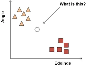
dogs, the circle and triangle are already classified by the two features of claws and sound, so what kind of star does this represent? The principle of KNN is shown in Figure 1(a) and Figure 1(b).
When k = 3, the three lines are the closest three points, so the circle is more, so the star belongs to the cat.
2.5. Logistic Regression
The logistic regression model is a two class model. It selects different features and weights to classify the samples, and calculates the probability of the samples belonging to a certain class with each log function. That is, a sample will have a certain probability, belong to a class, there will be a certain probability, belong to another class; the probability of large class is the sample belongs to the class.
2.6. Decision Tree
The decision tree is a predictive model that represents a mapping between object attributes and object values. It is classified according to the features, each node raises a problem, and the data are divided into two categories by judgment, and then continue to ask questions. These questions are learned from existing data, and when new data is added, the data can be partitioned into suitable leaves based on the tree’s problem.
2.7. Support Vector Machines (SVM)
Support vector machine (SVM) is a learning theory of VC dimension theory and structural risk minimization principle on the basis of statistics. According to the limited sample information in model complexity and learning ability, it will ob-tain the best generalization ability. SVM is a two classification algorithm, which can find a (N-1) dimension hyper plane in N dimension space. This hyper plane can classify these points into two categories. That is to say, if there are two classes of linearly separable points in the plane, SVM can find an optimal straight line separating these points.
2.8. Random Forest
[image:6.595.304.444.600.705.2]Random forest is based on decision tree. It is a classifier that combines existing classifiers algorithms in a certain way to form a classifier with stronger
DOI: 10.4236/ojbm.2018.61001 7 Open Journal of Business and Management
performance, and a weak classifier is assembled into a strong classifier. Its algo-rithm process is as follows:
1) Extract training sets from the original sample set. Each round extracts N training samples from the original sample using Bootstraping (In the training set, some samples may be extracted several times, while some samples may not be extracted at one time). K rounds were extracted and k independent training sets were obtained;
2) K decision tree models are obtained through K training sets;
3) K decision tree model is adopted to get the classification results by voting. the importance of all models is the same.
3. Data Selection
3.1. Data-Set
In this paper, the data set is collected from the Wind Financial Terminal Data-base and CCER Economic and Financial database. It contains all kinds of finan-cial data of capital market enterprises which being disclosed by the finanfinan-cial statements. In China, if the listed company loses two consecutive years, it will be marked ST. In addition, the company that has been losing money for three years will be marked *ST. Such companies would be in danger of exiting the capital markets. In order to assess the reliability of the method, we are going to draw random sampling financial data covering 2000 to 2016 on China capital market companies. In this paper, we will take the company of ST as the bankruptcy sample and the company of net profit for four years is positive as the non-bankruptcy sample. The process of data selection follows the following proceeds:
First of all, in China, financial industry and non-financial industry follows the different accounting standards. So there are some differences in accounting statements and we need to distinguish two kinds of industry. However, financial industry have too much uncertainty mainly based on the national policies and regulations, so it has the high risk, therefore we decided to analyze non-financial industry.
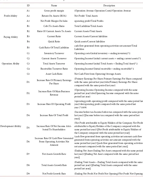
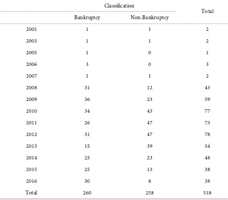
Next, it is necessary to choose the indicators to evaluate the enterprise. From the financial management perspective, the enterprise evaluation mainly consists of the following four abilities: Debt Paying ability, Operation ability, Profit abili-ty and Development abiliabili-ty. Moreover, different abiliabili-ty measurement system has different index composition. The indicators considered in the paper are de-scribed in details in Table 1. After the above steps, 518 companies are selected as samples. The numbers of observation in each year are shown in Table 2.
3.2. Data Filtering Results
To reduce the computational complexity and improve the significance of the model, it is necessary to make a significance test and filter candidate indicator variables. The proceeds of filter are as follows:
DOI: 10.4236/ojbm.2018.61001 8 Open Journal of Business and Management Table 1. The set of indicators considered in classification process.
ID Name Description
Profit Ability
A1 Gross profit margin (Operation Avenue-Operation Costs)/Operation Avenue A2 Return On Assets (ROA) Net Profit/ Total Assets
A3 Net Profit Margin On Sales operating profit/Total Profits
Paying Ability
B1 Cebt To Assets Ratio Total Liabilities/Total Assets B2 Ratio Of Current Assets To Assets Current Assets/Total Assets B3 Current Ratio Current Assets/Current liabilities B4 Quick Ratio Quick assets/Current liabilities
B5 Cash Ratio Of Total Liabilities cash flow generated from operating activities net amount/Total Liabilities
Operation Ability
C1 Inventory Turnover Operating costs/(initial inventory + ending inventory)*2
C2 Current Assets Turnover Operating Income/(initial current assets + ending current assets)*2 C3 Total Assets Turnover Operating Income/(initial Total Assets + Ending Total Asset)*2 C4 Receivables Turnover Ratio Operating Income/(Initial receivable + ending receivable)*2 C5 Asset Cash Ratio Net Cash Flow from Operating/Average Assets
Development Ability
D1 Increase Rate Of Primary Earnings Per Share (Primary Earnings Per Share-Primary Earnings Per Share compared with the same period last year)/abs(Primary Earnings Per Share compared with the same period last year)
D2 Increase Rate Of Main Business Revenue (Operating Income-Operating Income compared with the same period last year)/abs(Operating Income compared with the same period last year)
D3 Increase Rate Of Operating Profit (operating profit-operating profit compared with the same period last year)/abs(operating profit compared with the same period last year )*100%
D4 Increase Rate Of Total Profit (Income before tax-Income before tax compared with the same period last year)/||Income before tax compared with the same period last year||
D5 Increase Rate Of Net Income Attri-buted To Shareholders
(Net Profit attributable to Equity Holders of the Company-Net Profit attributable to Equity Holders of the Company compared with the same period last year)/||Net Profit attributable to Equity Holders of the Company compared with the same period last year||
D6 Increase Rate Of Cash Flow Generated From Operating Activities Net Amount
(cash flow generated from operating activities net amount-cash flow generated from operating activities net amount compared with the same period last year)/||cash flow generated from operating activities net amount compared with the same period last year||
D7 Net Assets Growth Rate (Ending Net Asset-Ending Net Asset compared with the same period last year)/||Ending Net Asset compared with the same period last year||
D8 Total Assets Growth Rate (Ending Total Assets---Ending Total Assets compared with the same period last year)/||Ending Total Assets compared with the same period last year||
D9 Net Profit Growth Rate (Ending Net Profit-Net Profit Not Opening)/Net Profit Not Opening
DOI: 10.4236/ojbm.2018.61001 9 Open Journal of Business and Management Table 2. The number of observations of different types of samples in each observed years.
Classification
Total Bankruptcy Non-Bankruptcy
2001 1 1 2
2003 1 1 2
2005 1 0 1
2006 3 0 3
2007 1 1 2
2008 31 12 43
2009 36 23 59
2010 34 43 77
2011 26 47 73
2012 31 47 78
2013 15 39 54
2014 25 23 48
2015 25 13 38
2016 30 8 38
Total 260 258 518
Wilcoxon rank and perform non-parametric test. In the end, according to the standard of certain significance level, the model variables will be determined. In this paper, stata 10.0 is selected as the data statistics software. Stata is widely used in data analysis and it provides everything researchers need for statistics, graphics, and data management.
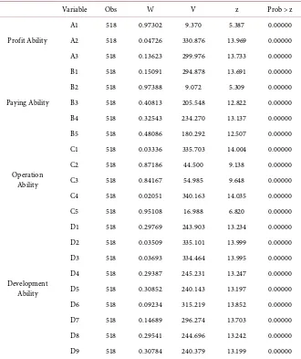
There are many methods to check the normal distribution. Different methods apply to different sample characteristic. Based on the sample of the paper, we choose Shapiro-Wilk test as a method. Shapiro-Wilk test is applicable to normal distribution test of sample size less than 2000. Besides, it is widely used in ex-plore the distribution of continuous random variables. The selected financial in-dicators are inspected and the results are shown in the Table 3.
DOI: 10.4236/ojbm.2018.61001 10 Open Journal of Business and Management Table 3. Normal distribution test results.
Variable Obs W V z Prob > z
Profit Ability
A1 518 0.97302 9.370 5.387 0.00000
A2 518 0.04726 330.876 13.969 0.00000 A3 518 0.13623 299.976 13.733 0.00000
Paying Ability
B1 518 0.15091 294.878 13.691 0.00000
B2 518 0.97388 9.072 5.309 0.00000
B3 518 0.40813 205.548 12.822 0.00000 B4 518 0.32543 234.270 13.137 0.00000 B5 518 0.48086 180.292 12.507 0.00000
Operation Ability
C1 518 0.03336 335.703 14.004 0.00000 C2 518 0.87186 44.500 9.138 0.00000 C3 518 0.84167 54.985 9.648 0.00000 C4 518 0.02051 340.163 14.035 0.00000 C5 518 0.95108 16.988 6.820 0.00000
Development Ability
D1 518 0.29769 243.903 13.234 0.00000 D2 518 0.03509 335.101 13.999 0.00000 D3 518 0.03693 334.464 13.995 0.00000 D4 518 0.29387 245.231 13.247 0.00000 D5 518 0.30852 240.143 13.197 0.00000 D6 518 0.09234 315.219 13.852 0.00000 D7 518 0.14689 296.274 13.703 0.00000 D8 518 0.29541 244.696 13.242 0.00000 D9 518 0.30784 240.379 13.199 0.00000
less than 0.05, so we can make a decision that all indicators are not subject to normal distribution. After the normal distribution test, the difference signific-ance test method should be selected according to the test results. The normal test results of this paper can be seen that all indicators require non-parametric test. The test results are shown in the Table 4.
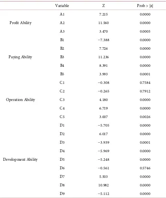
DOI: 10.4236/ojbm.2018.61001 11 Open Journal of Business and Management Table 4. Non-Parametric test results.
Variable Z Prob > |z|
Profit Ability
A1 7.215 0.0000
A2 11.560 0.0000
A3 3.470 0.0005
Paying Ability
B1 −7.388 0.0000
B2 7.726 0.0000
B3 11.236 0.0000
B4 8.391 0.0000
B5 3.993 0.0001
Operation Ability
C1 −0.308 0.7584
C2 −0.265 0.7912
C3 4.180 0.0000
C4 6.719 0.0000
C5 3.007 0.0026
Development Ability
D1 −5.705 0.0000
D2 6.017 0.0000
D3 −3.939 0.0001
D4 −5.969 0.0000
D5 −5.248 0.0000
D6 −0.561 0.5746
D7 5.503 0.0000
D8 10.982 0.0000
D9 −5.112 0.0000
0.05, so the financial indicators can be distinguished significantly and needs to be retained as the test financial indicator. Through the above index analysis process, the final selected sample index is A1. A2 and A3 in Profit ability, B1. B2. B3. B4 and B5 in paying ability, C3. C4 and C5 in operation ability, D1. D2. D3. D4. D5. D7. D8 and D9 in development ability.
4. Experiments
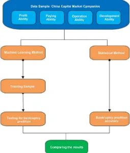
After data filtering, it is necessary to conduct the experiment. In this section, we will take both statistical and machine learning methods to predict bankruptcy.
Figure 2 illustrates our methodology.
DOI: 10.4236/ojbm.2018.61001 12 Open Journal of Business and Management Figure 2. The structure of this paper.
train data, so we will choose the proper train set. After the process of learning, we will take test set to complete bankruptcy prediction. After the experiment, we will compare the accuracy of two methods and determine which method is more accurate.
4.1. Statistical Method
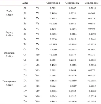
In this section, we will take statistical method to conduct bankruptcy prediction. The bankruptcy prediction of statistical methods is mainly composed of the fol-lowing steps: Firstly, it is necessary to analyze the principal component of four financial analysis indicators. Secondly, the binary logistic regression analysis is used to predict the bankruptcy. The results of Principle Components Analysis can be seen in Table 5.
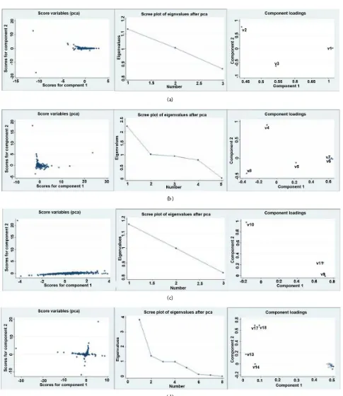
In this section, we conducted principal component analysis on four financial indicators. After principal component analysis, we extracted the first principal components as a comprehensive evaluation of each financial index. During the period of principle component analysis, the gravel figure, score figure and load-ing figure of each variable are shown in Figure 3.
Figure 3 shows the gravel figure, score figure and loading figure of each
DOI: 10.4236/ojbm.2018.61001 13 Open Journal of Business and Management Table 5. The results of principal component analysis.
Label Component 1 Component 2 Component 3
Profit Ability
A1 V1 0.7131 0.0067 −0.7010
A2 V2 0.4418 0.7721 0.4568
A3 V3 0.5443 −0.6355 0.5476
Paying Ability
B1 V4 −0.1081 0.9011 0.0556
B2 V5 0.2245 −0.1244 0.9403
B3 V6 0.6473 −0.0274 −0.1398
B4 V7 0.6330 0.0010 −0.2641
B5 V8 −0.3438 −0.4144 −0.1528
Operation Ability
C3 V9 0.7080 −0.0103 0.7061
C4 V10 −0.1588 0.9179 0.1735
C5 V11 0.6881 0.2350 −0.6865
Development Ability
D1 V12 0.4969 −0.0972 −0.0128
D2 V13 0.0191 0.1654 0.8772
D3 V14 0.0697 −0.0026 0.4481
D4 V15 0.4878 −0.0360 −0.0185
D5 V16 0.5021 −0.0519 −0.0153
D7 V17 0.0683 0.6923 −0.1608
D8 V18 0.0943 0.6912 −0.0524
D9 V19 0.4943 −0.0476 −0.0183
components, V1 plays a major part and V2 plays the weakest role. From the gravel figure, we can see that eigenvalues greater than 1 consists of the first prin-cipal component and the second prinprin-cipal component. Therefore, according to the above analysis, we select the first principal component as an indicator of profit ability. Based on the above analysis process, we confirm that the first prin-cipal component is used as a measure of paying ability. Operation ability and development ability. After the dimension reduction of various financial tors, four comprehensive abilities are formed to measure four financial indica-tors, respectively F1 F2 F3 and F4 the comprehensive evaluation ability of each financial index is as follows:
1 0.7131 1 0.4418 2 0.5443 3
F = ∗A + ∗A + ∗A
2 0.1081 1 0.2245 2 0.6473 3 0.6330 4 0.3438 5
F = − ∗B + ∗B + ∗B + ∗B − ∗B
3 0.7080 3 0.1588 4 0.6881 5
F = ∗C − ∗C + ∗C
4 0.4969 1 0.0191 2 0.0697 3 0.4878 4 0.5021 5
0.0683 7 0.0943 8 0.4943 9
F D D D D D
D D D
= ∗ + ∗ + ∗ + ∗ + ∗
+ ∗ + ∗ + ∗
where
DOI: 10.4236/ojbm.2018.61001 14 Open Journal of Business and Management (a)
(b)
(c)
[image:14.595.57.542.59.618.2](d)
Figure 3. The gravel figure, score figure and loading figure of each variable. (a) Profit ability; (b) Paying ability; (c) Paying ability; (d) Development ability.
F3 is the comprehensive evaluation of operation ability; F4 is the comprehensive evaluation of development ability.
DOI: 10.4236/ojbm.2018.61001 15 Open Journal of Business and Management
[image:15.595.205.541.637.730.2]F2 F3 and F4 respectively. The results of bankruptcy prediction can be seen in
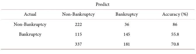
Table 6.
From Table 6, we can draw the following conclusions: The Non-bankruptcy prediction probability of the enterprise is 86% and bankruptcy prediction prob-ability of the enterprise is 55.8%. Therefore, the probprob-ability of accurate predic-tion is 70.8%. This probability is consistent with the exact probability of the most financial model predictions. However, the prediction accuracy of this model is not high and needs to be improved.
4.2. Machine Learning Methods
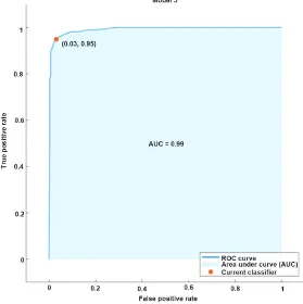
After the statistical method, we will take machine learning methods to take bankruptcy prediction. In this section, we choose KNN. SVM. Logistic regres-sion. Random forest and decision tree to forecast bankruptcy. Figure 2 shows the ROC (Receiver Operating Characteristic) curve of random forest model.
From Figure 4, we can draw the conclusion that random forest model shows the outstanding accuracy. The square of the shaded area has reached 0.99, which is close to the largest area 1. The shaded area shows the diagnosis effect. The bigger the shadow, the better the diagnosis effect. Besides, in order to verify the effectiveness of more machine learning methods, we enumerated the confusion matrix of five machine learning methods. The confusion matrix of five machine learning methods can be seen in Figure 5.
Figure 5 shows the bankruptcy prediction outcomes for machine learning
methods. The random forest and decision tree shows high accuracy with 95% and 94% in non-bankruptcy prediction. Besides, the KNN. SVM and logistic re-gression have the lower accuracy with 88% 88% and 84% respectively. However, compared to statistical method with 86%, four machine learning methods have the higher predictive accuracy except for logistic regression. As for bankruptcy prediction, machine learning methods show significant superiority over statis-tical method. The random forest shows the highest accuracy with 97% and the KNN shows the lowest accuracy with 74% which is much greater than statistical method with 55.8%. In addition, the remaining fours machine learning methods also have high prediction accuracy than statistical method.
In conclusion, the machine learning method has the higher bankruptcy pre-diction accuracy than statistical method. Overall results of different methods can be seen in Figure 6. The prediction of random forest is 95.9%. It is clear that
Table 6. The results of bankruptcy prediction.
Predict
Actual Non-Bankruptcy Bankruptcy Accuracy (%)
Non-Bankruptcy 222 36 86
Bankruptcy 115 145 55.8
DOI: 10.4236/ojbm.2018.61001 16 Open Journal of Business and Management Figure 4. ROC curve of random forest model to predict bankruptcy, with
data from China capital market listed companies.
(a)
DOI: 10.4236/ojbm.2018.61001 17 Open Journal of Business and Management (d) (e)
Figure 5. Confusion matrix of each machine learning method. (a) Bankruptcy prediction of KNN; (b) Bankruptcy prediction of SVM; (c) Bankruptcy prediction of Logistic R; (d) Bankruptcy prediction of Random Forest; (e) Bankruptcy prediction of Deci-sion Tree.
Figure 6. Overall results of different methods.
machine learning method is more accurate than other prediction method. The results demonstrate that machine learning method has the advantage to predict bankruptcy over the statistical method.
5. Conclusions
This paper compares the accuracy of statistical forecasting and machine learning methods to predict bankruptcy in Chinese-listed companies. Firstly, we take Shapiro-Wilk test to test the normal distribution. Secondly, according to the Shapiro-Wilk test result, it is necessary to determine the parameter test or the non-parametric test. In the end, we take both statistical method and machine learning method we predict bankruptcy. The empirical results show that ma-chine learning methods are superior to statistical methods.
[image:17.595.154.441.288.481.2]DOI: 10.4236/ojbm.2018.61001 18 Open Journal of Business and Management
measurement of financial indicators, we carry out binary logistic regression to four comprehensive indexes. The final rate of accuracy is 70.8%. However, each machine learning method (KNN, SVM, Logistic Regression, Decision Tree, and Random Forest) has the greater accuracy than statistical method.
In the future, we plan to extend our work to more indicators of the compa-nies. With the development of the China capital market, there will be more company characteristics to be disclosure. Based on this trend, we will select more indicators to predict bankruptcy. Furthermore, we will apply the method to more small and medium enterprise in China. Subsequently, we would try more machine learning method and improve the accuracy of bankruptcy prediction.
References
[1] Altman, E.I. (1968) Financial Ratios, Discriminant Analysis and the Prediction of Corporate Bankruptcy. Journal of Finance, 23, 589-609.
https://doi.org/10.1111/j.1540-6261.1968.tb00843.x
[2] Fitzpatrick, P.J. (1932) A Comparison of the Ratios of Successful Industrial Enter-prises with Those of Failed Companies. Análise Molecular Do Gene Wwox, 598-605.
[3] Smith, R. and Winakor, A. (1935) Changes in the Financial Structure of Unsuccess-ful Corporations.
[4] Merwin, C.L. (1942) Financing Small Corporations in Five Manufacturing Indus-tries, 1926-1936: A Dissertation in Economics. Financing Small Corporations in Five Manufacturing Industries, 1926-36. National Bureau of Economic Research. [5] Beaver, W.H. (1966) Financial Ratios as Predictors of Failure. Journal of
Account-ing Research, 4, 71-111.https://doi.org/10.2307/2490171
[6] Ohlson, J.A. (1980) Financial Ratios and the Probabilistic Prediction of Bankruptcy.
Journal of Accounting Research, 18, 109-131.https://doi.org/10.2307/2490395 [7] West, R.C. (1985) A Factor-Analytic Approach to Bank Condition. Journal of
Banking & Finance, 9, 253-266.https://doi.org/10.1016/0378-4266(85)90021-4 [8] Aziz, A., Emanuel, D.C. and Lawson, G.H. (1988) Bankruptcy Prediction—An
In-vestigation of Cash Flow Based Models. Journal of Management Studies, 25, 419-437.https://doi.org/10.1111/j.1467-6486.1988.tb00708.x
[9] Koh, H.C. and Killough, L.N. (2010) The Use of Multiple Discriminant Analysis in the Assessment of the Going-Concern Status of an Audit Client. Journal of Business Finance & Accounting, 17, 179-192.
https://doi.org/10.1111/j.1468-5957.1990.tb00556.x
[10] Platt, H.D., Platt, M.B. and Pedersen, J.G. (1994) Bankruptcy Discrimination with Real Variables. Journal of Business Finance & Accounting, 21, 491-510.
https://doi.org/10.1111/j.1468-5957.1994.tb00332.x
[11] Upneja, A. and Dalbor, M.C. (2000) An Examination of Capital Structure in the Restaurant Industry. International Journal of Contemporary Hospitality Manage-ment, 13, 54-59.https://doi.org/10.1108/09596110110381825
[12] Beaver, W.H., Mcnichols, M.F. and Rhie, J.W. (2005) Have Financial Statements Become Less Informative? Evidence from the Ability of Financial Ratios to Predict Bankruptcy. Review of Accounting Studies, 10, 93-122.
DOI: 10.4236/ojbm.2018.61001 19 Open Journal of Business and Management [13] Subasi, A. and Gursoy, M.I. (2010) Eeg Signal Classification Using pca, ica, lda and
Support Vector Machines. Expert Systems with Applications, 37, 8659-8666. https://doi.org/10.1016/j.eswa.2010.06.065
[14] Menezes, F.S.D., Liska, G.R., Cirillo, M.A. and Vivanco, M.J.F. (2016) Data Classi-fication with Binary Response through the Boosting Algorithm and Logistic Regres-sion. Expert Systems with Applications, 69, 62-73.
https://doi.org/10.1016/j.eswa.2016.08.014
[15] Maione, C., Paula, E.S.D., Gallimberti, M., Batista, B.L., Campiglia, A.D., Jr, F.B., et al. (2016) Comparative Study of Data Mining Techniques for the Authentication of Organic Grape Juice Based on icp-ms Analysis. Expert Systems with Applications, 49, 60-73.https://doi.org/10.1016/j.eswa.2015.11.024
[16] Cano, G., Garcia-Rodriguez, J., Garcia-Garcia, A., Perez-Sanchez, H., Benediktsson, J.A., Thapa, A., et al. (2016) Automatic Selection of Molecular Descriptors using Random Forest: Application to Drug Discovery. Expert Systems with Applications. [17] Heo, J. and Yang, J.Y. (2014) Adaboost Based Bankruptcy Forecasting of Korean
Construction Companies. Applied Soft Computing, 24, 494-499. https://doi.org/10.1016/j.asoc.2014.08.009
[18] Kim, M.J., Kang, D.K. and Hong, B.K. (2015) Geometric Mean Based Boosting Al-gorithm with Over-Sampling to Resolve Data Imbalance Problem for Bankruptcy Prediction. Expert Systems with Applications, 42, 1074-1082.
https://doi.org/10.1016/j.eswa.2014.08.025
[19] Wilson, R.L. and Sharda, R. (1994) Bankruptcy Prediction Using Neural Networks.
Decision Support Systems, 11, 545-557. https://doi.org/10.1016/0167-9236(94)90024-8
[20] Tsai, C.F. (2008) Financial Decision Support using Neural Networks and Support Vector Machines. Expert Systems, 25, 380-393.
https://doi.org/10.1111/j.1468-0394.2008.00449.x
[21] Chen, M.Y. (2011) Predicting Corporate Financial Distress Based on Integration of Decision Tree Classification and Logistic Regression. Expert Systems with Applica-tions, 38, 11261-11272.https://doi.org/10.1016/j.eswa.2011.02.173
[22] Cho, S., Hong, H. and Ha, B.C. (2010) A Hybrid Approach Based on the Combina-tion of Variable SelecCombina-tion using Decision Trees and Case-Based Reasoning using the Mahalanobis Distance: For Bankruptcy Prediction. Expert Systems with Applica-tions, 37, 3482-3488.https://doi.org/10.1016/j.eswa.2009.10.040
[23] Chen, H.J., Huang, S.Y. and Lin, C.S. (2009) Alternative Diagnosis of Corporate Bankruptcy: A Neuro Fuzzy Approach. Expert Systems with Applications, 36, 7710-7720.https://doi.org/10.1016/j.eswa.2008.09.023
[24] Cortes, C. and Vapnik, V. (1995) Support-Vector Networks. Machine Learning, 20, 273-297.https://doi.org/10.1007/BF00994018
[25] Shin, K.S., Lee, T.S. and Kim, H.J. (2005) An Application of Support Vector Ma-chines in Bankruptcy Prediction Model. Expert Systems with Applications, 28, 127-135.https://doi.org/10.1016/j.eswa.2004.08.009
[26] Chaudhuri, A. and De, K. (2011) Fuzzy Support Vector Machine for Bankruptcy Prediction. Applied Soft Computing Journal, 11, 2472-2486.
https://doi.org/10.1016/j.asoc.2010.10.003
DOI: 10.4236/ojbm.2018.61001 20 Open Journal of Business and Management https://doi.org/10.1016/j.asoc.2012.03.028
[28] Zhou, L., Lai, K.K. and Yu, L. (2009) Credit Scoring using Support Vector Machines with Direct Search for Parameters Selection. Soft Computing, 13, 149.
https://doi.org/10.1007/s00500-008-0305-0