Trans-dimensional Random Fields for Language Modeling
Bin Wang1, Zhijian Ou1, Zhiqiang Tan2
1Department of Electronic Engineering, Tsinghua University, Beijing 100084, China 2Department of Statistics, Rutgers University, Piscataway, NJ 08854, USA [email protected], [email protected],
Abstract
Language modeling (LM) involves determining the joint probability of words in a sentence. The conditional approach is dominant, representing the joint probability in terms of conditionals. Examples include n-gram LMs and neural network LMs. An alternative approach, called the random field (RF) approach, is used in whole-sentence maximum entropy (WSME) LMs. Although the RF approach has potential benefits, the empirical results of previous WSME models are not satisfactory. In this paper, we revisit the RF approach for language modeling,
with a number of innovations. We
propose a trans-dimensional RF (TDRF) model and develop a training algorithm using joint stochastic approximation and trans-dimensional mixture sampling. We perform speech recognition experiments on Wall Street Journal data, and find that our TDRF models lead to performances as good as the recurrent neural network LMs but are computationally more efficient in computing sentence probability.
1 Introduction
Language modeling is crucial for a variety of computational linguistic applications, such as speech recognition, machine translation, handwriting recognition, information retrieval and so on. It involves determining the joint probability p(x) of a sentence x, which can be denoted as a pair x = (l, xl), where l is the length and
xl = (x1, . . . , xl)is a sequence oflwords.
Currently, the dominant approach is conditional modeling, which decomposes the joint probability ofxl into a product of conditional probabilities1
1And the joint probability of xis modeled asp(x) =
by using the chain rule,
p(x1, . . . , xl) = l
Y
i=1
p(xi|x1, . . . , xi−1). (1)
To avoid degenerate representation of the con-ditionals, the history of xi, denoted as hi =
(x1,· · · , xi−1), is reduced to equivalence classes
through a mappingφ(hi)with the assumption
p(xi|hi)≈p(xi|φ(hi)). (2)
Language modeling in this conditional approach consists of finding suitable mappings φ(hi) and effective methods to estimate
p(xi|φ(hi)). A classic example is the traditional
n-gram LMs with φ(hi) = (xi−n+1, . . . , xi−1).
Various smoothing techniques are used for parameter estimation (Chen and Goodman, 1999). Recently, neural network LMs, which have begun to surpass the traditionaln-gram LMs, also follow the conditional modeling approach, with φ(hi)
determined by a neural network (NN), which can be either a feedforward NN (Schwenk, 2007) or a recurrent NN (Mikolov et al., 2011).
Remarkably, an alternative approach is used in whole-sentence maximum entropy (WSME) lan-guage modeling (Rosenfeld et al., 2001). Specifi-cally, a WSME model has the form:
p(x;λ) = Z1 exp{λTf(x)} (3)
Here f(x) is a vector of features, which can be arbitrary computable functions ofx,λis the cor-responding parameter vector, andZ is the global normalization constant. Although WSME mod-els have the potential benefits of being able to naturally express sentence-level phenomena and integrate features from a variety of knowledge p(xl)p(hEOSi|xl), wherehEOSiis a special token placed at the end of every sentence. Thus the distribution of the sentence length is implicitly modeled.
sources, their performance results ever reported are not satisfactory (Rosenfeld et al., 2001; Amaya and Bened´ı, 2001; Ruokolainen et al., 2010).
The WSME model defined in (3) is basically a Markov random field (MRF). A substantial chal-lenge in fitting MRFs is that evaluating the gradi-ent of the log likelihood requires high-dimensional integration and hence is difficult even for mod-erately sized models (Younes, 1989), let alone the language model (3). The sampling methods previously tried for approximating the gradient are the Gibbs sampling, the Independence Metropolis-Hasting sampling and the importance sampling (Rosenfeld et al., 2001). Simple applications of these methods are hardly able to work efficient-ly for the complex, high-dimensional distribution such as (3), and hence the WSME models are in fact poorly fitted to the data. This is one of the reasons for the unsatisfactory results of previous WSME models.
In this paper, we propose a new language model, called the trans-dimensional random field (TDRF) model, by explicitly taking account of the empirical distributions of lengths. This formulation subsequently enables us to develop a powerful Markov chain Monte Carlo (MCMC) technique, called trans-dimensional mixture sampling and then propose an effective training algorithm in the framework of stochastic approximation (SA) (Benveniste et al., 1990; Chen, 2002). The SA algorithm involves jointly updating the model parameters and normalization constants, in conjunction with trans-dimensional MCMC sampling. Section 2 and 3 present the model definition and estimation respectively.
Furthermore, we make several additional in-novations, as detailed in Section 4, to enable successful training of TDRF models. First, the diagonal elements of hessian matrix are estimat-ed during SA iterations to rescale the gradient, which significantly improves the convergence of the SA algorithm. Second, word classing is in-troduced to accelerate the sampling operation and also improve the smoothing behavior of the mod-els through sharing statistical strength between similar words. Finally, multiple CPUs are used to parallelize the training of our RF models.
In Section 5, speech recognition experiments are conducted to evaluate our TDRF LMs, com-pared with the traditional 4-gram LMs and the re-current neural network LMs (RNNLMs) (Mikolov
et al., 2011) which have emerged as a new state-of-art of language modeling. We explore the use of a variety of features based on word and class information in TDRF LMs. In terms of word error rates (WERs) for speech recognition, our TDRF LMs alone can outperform the KN-smoothing 4-gram LM with 9.1% relative reduction, and per-form comparably to the RNNLM with a slight 0.5% relative reduction. To our knowledge, this result represents the first strong empirical evidence supporting the power of using the whole-sentence language modeling approach. Our open-source TDRF toolkit is released publicly2.
2 Model Definition
Throughout, we denote 3 byxl = (x1, . . . , xl) a
sentence (i.e., word sequence) of lengthlranging from 1 tom. Each element of xl corresponds to
a single word. For l = 1, . . . , m, we assume that sentences of lengthl are distributed from an exponential family model:
pl(xl;λ) = Z1 l(λ)e
λTf(xl)
, (4)
where f(xl) = (f
1(xl), f2(xl), . . . , fd(xl))T is
the feature vector and λ = (λ1, λ2, . . . , λd)T is
the corresponding parameter vector, andZl(λ)is
the normalization constant:
Zl(λ) =
X
xl
eλTf(xl) (5)
Moreover, we assume that length l is associated with probability πl forl = 1, . . . , m. Therefore,
the pair(l, xl)is jointly distributed as
p(l, xl;λ) =π
lpl(xl;λ). (6)
We provide several comments on the above model definition. First, by making explicit the role of lengths in model definition, it is clear that the model in (6) is a mixture of random fields on sentences of different lengths (namely on sub-spaces of different dimensions), and hence will be called a trans-dimensional random field (TDRF). Different from the WSME model (3), a crucial aspect of the TDRF model (6) is that the mixture weights πl can be set to the empirical length
probabilities in the training data. The WSME
2http://oa.ee.tsinghua.edu.cn/
˜ouzhijian/software.htm
model (3) is essentially also a mixture of RFs, but the mixture weights implied are proportional to the normalizing constantsZl(λ):
p(l, xl;λ) = ZZl((λλ))Z1
l(λ)e λTf(xl)
, (7)
whereZ(λ) =Pml=1Zl(λ).
A motivation for proposing (6) is that it is very difficult to sample from (3), namely (7), as a mixture distribution with unknown weights which typically differ from each other by orders of magnitudes, e.g.1040or more in our experiments.
Setting mixture weights to the known, empirical length probabilities enables us to develop a very effective learning algorithm, as introduced in Sec-tion 3. Basically, the empirical weights serve as a control device to improve sampling from multiple distributions (Liang et al., 2007; Tan, 2015) .
Second, it can be shown that if we incorporate the length features4in the vector of featuresf(x)
in (3), then the distribution p(x;λ) in (3) under the maximum entropy (ME) principle will take the form of (6) and the probabilities(π1, . . . , πm) in
(6) implied by the parameters for the length fea-tures are exactly the empirical length probabilities. Third, a feature fi(xl),1 ≤ i ≤ d, can be any
computable function of the sentence xl, such as
n-grams. In our current experiments, the features fi(xl) and their corresponding parametersλi are
defined to be position-independent and length-independent. For example,fi(xl) =Pkfi(xl, k),
wherefi(xl, k)is a binary function ofxlevaluated
at positionk. As a result, the featurefi(xl)takes
values in the non-negative integers.
3 Model Estimation
We develop a stochastic approximation algorith-m using Markov chain Monte Carlo to estialgorith-mate the parametersλand the normalization constants Z1(λ), ..., Zm(λ) (Benveniste et al., 1990; Chen,
2002). The core algorithms newly designed in this paper are the joint SA for simultaneously estimating parameters and normalizing constants (Section 3.2) and trans-dimensional mixture sam-pling (Section 3.3) which is used as Step I of the joint SA. The most relevant previous works that we borrowed from are (Gu and Zhu, 2001) on SA for fitting a single RF, (Tan, 2015) on sampling and
4The length feature corresponding to lengthlis a binary
feature that takes one if the sentencexis of length l, and otherwise takes zero.
estimating normalizing constants from multiple RFs of the same dimension, and (Green, 1995) on trans-dimensional MCMC.
3.1 Maximum likelihood estimation
Suppose that the training dataset consists of nl
sentences of length l for l = 1, . . . , m. First, the maximum likelihood estimate of the length probabilityπl is easily shown to be nl/n, where
n = Pml=1nl. By abuse of notation, we set
πl = nl/n hereafter. Next, the log-likelihood of
λgiven the empirical length probabilities is
L(λ) = 1nXm
l=1
X
xl∈Dl
logpl(xl;λ), (8)
whereDlis the collection of sentences of lengthl
in the training set. By setting to 0 the derivative of (8) with respect toλ, we obtain that the maximum likelihood estimate of λ is determined by the following equation:
∂L(λ)
∂λ = ˜p[f]−pλ[f] = 0, (9) wherep˜[f]is the expectation of the feature vector f with respect to the empirical distribution:
˜ p[f] = 1
n
m
X
l=1
X
xl∈Dl
f(xl), (10)
andpλ[f]is the expectation off with respect to
the joint distribution (6) withπl=nl/n:
pλ[f] = m
X
l=1
nl
npλ,l[f], (11)
and pλ,l[f] = Pxlf(xl)pl(xl;λ). Eq.(9) has
the form of equating empirical expectations p˜[f] with theoretical expectations pλ[f], as similarly
found in maximum likelihood estimation of single random field models.
3.2 Joint stochastic approximation
Training random field models is challenging due to numerical intractability of the normalizing con-stantsZl(λ)and expectationspλ,l[f]. We propose
a novel SA algorithm for estimating the parame-tersλ by (9) and, simultaneously, estimating the log ratios of normalization constants:
ζl∗(λ) = logZZl(λ)
Algorithm 1Joint stochastic approximation Input: training set
1: set initial valuesλ(0)= (0, . . . ,0)Tand ζ(0)=ζ∗(λ(0))−ζ∗
1(λ(0))
2: fort= 1,2, . . . , tmaxdo
3: setB(t)=∅
4: set(L(t,0), X(t,0)) = (L(t−1,K), X(t−1,K)) Step I: MCMC sampling
5: fork= 1→Kdo
6: sampling (See Algorithm 3)
(L(t,k), X(t,k)) =SAMP LE(L(t,k−1), X(t,k−1))
7: setB(t)=B(t)∪ {(L(t,k), X(t,k))}
8: end for
Step II: SA updating
9: Computeλ(t)based on (14)
10: Computeζ(t)based on (15) and (16)
11: end for
whereZ1(λ)is chosen as the reference value and
can be calculated exactly. The algorithm can be obtained by combining the standard SA algorithm for training single random fields (Gu and Zhu, 2001) and a trans-dimensional extension of the self-adjusted mixture sampling algorithm (Tan, 2015).
Specifically, consider the following joint distri-bution of the pair(l, xl):
p(l, xl;λ, ζ)∝ eπζlleλTf(xl), (13)
where πl is set to nl/n for l = 1, . . . , m, but
ζ = (ζ1, . . . , ζm)T withζ1 = 0are hypothesized
values of the truthζ∗(λ) = (ζ∗
1(λ), . . . , ζm∗(λ))T
with ζ∗
1(λ) = 0. The distribution p(l, xl;λ, ζ)
reduces to p(l, xl;λ) in (6) if ζ were identical
to ζ∗(λ). In general, p(l, xl;λ, ζ) differs from
p(l, xl;λ) in that the marginal probability of
lengthlis not necessarilyπl.
The joint SA algorithm, whose pseudo-code is shown in Algorithm 1, consists of two steps at each timetas follows.
Step I: MCMC sampling. Generate a sample setB(t)withp(l, xl;λ(t−1), ζ(t−1))as the
station-ary distribution (see Section 3.3). Step II: SA updating.Compute
λ(t)=λ(t−1)+γλ
(
˜
p[f]−
P
(l,xl)∈B(t)f(xl)
K
)
(14)
whereγλis a learning rate ofλ; compute
ζ(t−12)=ζ(t)+γζ
δ
1(B(t))
π1 , . . . , δ
m(B(t)) πm
(15)
ζ(t)=ζ(t−21)−ζ(t−12)
1 (16)
whereγζis a learning rate ofζ, andδl(B(t))is the
relative frequency of lengthlappearing inB(t):
δl(B(t)) =
P
(j,xj)∈B(t)1(j=l)
K . (17)
The rationale in (15) is to adjust ζ based on how the relative frequencies of lengths δl(B(t))
are compared with the desired length probabili-ties πl. Intuitively, if the relative frequency of
some length l in the sample set B(t) is greater
(or respectively smaller) than the desired length probabilityπl, then the hypothesized value ζl(t−1)
is an underestimate (or overestimate) ofζ∗
l(λ(t−1))
and hence should be increased (or decreased). Following Gu & Zhu (2001) and Tan (2015), we set the learning rates in two stages:
γλ =
(
t−βλ ift≤t0
1
t−t0+tβλ0 ift > t0
(18)
γζ =
(
(0.1t)−βζ ift≤t0
1
0.1(t−t0)+(0.1t0)βζ ift > t0 (19)
where0.5< βλ, βζ <1. In the first stage (t≤t0),
a slow-decaying rate of t−β is used to introduce
large adjustments. This forces the estimates λ(t)
andζ(t)to fall reasonably fast into the true values.
In the second stage (t > t0), a fast-decaying
rate of t−1 is used. The iteration number t is
multiplied by 0.1 in (19), to make the the learning rate ofζ decay more slowly thanλ. Commonly, t0is selected to ensure there is no more significant
adjustment observed in the first stage. 3.3 Trans-dimensional mixture sampling We describe a trans-dimensional mixture sam-pling algorithm to simulate from the joint distri-bution p(l, xl;λ, ζ), which is used with(λ, ζ) =
(λ(t−1), ζ(t−1)) at time tfor MCMC sampling in
the joint SA algorithm. The name “mixture sam-pling” reflects the fact thatp(l, xl;λ, ζ)represents
a labeled mixture, becausel is a label indicating thatxlis associated with the distributionp
l(xl;ζ).
With fixed (λ, ζ), this sampling algorithm can be seen as formally equivalent to reversible jump MCMC (Green, 1995), which was originally pro-posed for Bayes model determination.
before sampling, but use the short notation(λ, ζ) for(λ(t−1), ζ(t−1)).
Step I: Local jump. The Metropolis-Hastings method is used in this step to sample the length. AssumingL(t−1) =k, first we draw a new length
j ∼ Γ(k,·). The jump distribution Γ(k, l) is defined to be uniform at the neighborhood ofk:
Γ(k, l) =
1
3, ifk∈[2, m−1], l∈[k−1, k+ 1] 1
2, ifk= 1, l∈[1,2]ork=m, l∈[m−1, m] 0, otherwise
(20)
wheremis the maximum length. Eq.(20) restricts the difference betweenjandkto be no more than one. Ifj=k, we retain the sequence and perform the next step directly, i.e. setL(t)=kandX(t) =
X(t−1). Ifj =k+ 1orj=k−1, the two cases
are processed differently.
If j = k + 1, we first draw an element (i.e., word) Y from a proposal distribution: Y ∼ gk+1(y|X(t−1)). Then we set
L(t)=j(=k+ 1)andX(t) ={X(t−1), Y}with
probability
min1,Γ(j, k)
Γ(k, j)
p(j,{X(t−1), Y};λ, ζ)
p(k, X(t−1);λ, ζ)gk+1(Y|X(t−1))
(21)
where{X(t−1), Y} denotes a sequence of length
k+ 1whose firstkelements are X(t−1) and the
last element isY.
If j = k−1, we set L(t) = j(= k−1)and
X(t) =X(t−1)
1:j with probability
min
(
1,Γ(Γ(j, kk, j))p(j, X
(t−1)
1:j ;λ, ζ)gk(Xk(t−1)|X1:(tj−1)) p(k, X(t−1);λ, ζ)
)
(22)
whereX1:(tj−1)is the firstjelements ofX(t−1)and
Xk(t−1)is thekth element ofX(t−1).
In (21) and (22), gk+1(y|xk) can be flexibly
specified as a proper density function iny. In our application, we find the following choice works reasonably well:
gk+1(y|xk) = p(k+ 1,{x
k, y};λ, ζ)
P
wp(k+ 1,{xk, w};λ, ζ). (23) Step II: Markov move. After the step of local jump, we obtain
X(t)=
X(t−1) ifL(t) =k {X(t−1), Y} ifL(t) =k+ 1
X1:(tk−−1)1 ifL(t) =k−1 (24)
Then we perform Gibbs sampling onX(t), from
the first element to the last element (Algorithm 2)
Algorithm 2Markov Move
1: fori= 1→L(t) do
2: drawW ∼p(L(t),{X(t)
1:i−1, w, Xi(+1:t) L(t)};λ, ζ) 3: setXi(t)=W
4: end for
4 Algorithm Optimization and Acceleration
The joint SA algorithm may still suffer from slow convergence, especially when λ is high-dimensional. We introduce several techniques for improving the convergence of the algorithm and reducing computational cost.
4.1 Improving SA recursion
We propose two techniques to effectively improve the convergence of SA recursion.
The first technique is to incorporate Hessian information, similarly as in related works on s-tochastic approximation (Gu and Zhu, 2001) and stochastic gradient descent algorithms (Byrd et al., 2014). But we only use the diagonal elements of the Hessian matrix to re-scale the gradient, due to high-dimensionality ofλ.
Taking the second derivatives ofL(λ)yields
Hi =−d
2L(λ)
dλ2
i =p[f
2
i]− m
X
l=1
πl(pl[fi])2 (25)
where Hi denotes the ith diagonal element of
Hessian matrix. At time t, before updating the parameterλ(Step II in Section 3.2), we compute
H(t−12)
i = K1
X
(l,xl)∈B(t)
fi(xl)2− m
X
l=1
πl(¯pl[fi])2,
(26) Hi(t)=Hi(t−1)+γH(H(t−
1 2)
i −Hi(t−1)), (27)
where p¯l[fi] = |Bl(t)|−1P(l,xl)∈B(t) l fi(x
l), and
Bl(t) is the subset, of size |B(lt)|, containing all sentences of lengthlinB(t).
The second technique is to introduce the “mini-batch” on the training set. At each iteration, a subsetD(t)ofKsentences are randomly selected
from the training set. Then the gradient is approx-imated with the overall empirical expectationp˜[f] being replaced by the empirical expectation over the subsetD(t). This technique is reminiscent of
0 20 40 60 80 100 120
140 160 180 200
t/10
− log−likelihood
without hessian with hessian
(a)
0 500 1000 1500 2000 50
100 150 200
t/10
negative log−likelihood
Hessian+mini−batch Hessian
[image:6.595.73.286.65.158.2](b)
Figure 1: Examples of convergence curves on training set after introducing hessian and training set mini-batching.
of optimization algorithms (Bousquet and Bottou, 2008).
By combining the two techniques, we revise the updating equation (14) ofλto
λ(t)
i =λ(it−1)+max(γλH(t)
i , h) ×
( P
(l,xl)∈D(t)fi(xl)
K −
P
(l,xl)∈B(t)fi(xl)
K
) (28)
where 0 < h < 1 is a threshold to avoid Hi(t) being too small or even zero. Moreover, a constant tcis added to the denominator of (18), to avoid too
large adjustment ofλ, i.e.
γλ =
( 1
tc+tβλ ift≤t0,
1
tc+t−t0+tβλ0 ift > t0.
(29)
Fig.1(a) shows the result after introducing hessian estimation, and Fig.1(b) shows the effect of train-ing set mini-batchtrain-ing.
4.2 Sampling acceleration
For MCMC sampling in Section 3.3, the Gibbs sampling operation of drawingXi(t)(Step 2 in Al-gorithms 2) involves calculating the probabilities of all the possible elements in position i. This is computationally costly, because the vocabulary size |V| is usually 10 thousands or more in prac-tice. As a result, the Gibbs sampling operation presents a bottleneck limiting the efficiency of sampling algorithms.
We propose a novel method of using class in-formation to effectively reduce the computational cost of Gibbs sampling. Suppose that each word in vocabulary V is assigned to a single class. If the total class number is |C|, then there are, on average, |V|/|C| words in each class. With the class information, we can first draw the class of Xi(t), denoted by c(it), and then draw a word
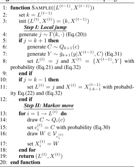
Algorithm 3Class-based MCMC sampling
1: functionSAMPLE((L(t−1), X(t−1)))
2: setk=L(t−1)
3: init(L(t), X(t)) = (k, X(t−1)) Step I: Local jump
4: generatej∼Γ(k,·)(Eq.(20)) 5: ifj=k+ 1then
6: generateC∼Qk+1(c)
7: generateY ∼˘gk+1(y|X(t−1), C)(Eq.31)
8: setL(t) = j andX(t) = {X(t−1), Y}with
probability (Eq.21) and (Eq.32) 9: end if
10: ifj=k−1then
11: setL(t) =jandX(t)=X(t−1)
1:k−1with
probabil-ity Eq.(22) and (Eq.32) 12: end if
Step II: Markov move
13: fori= 1→L(t) do
14: drawC∼Qi(c)
15: setc(it)=Cwith probability (Eq.30) 16: drawW ∈ Vc(t)
i 17: setX(t)
i =W 18: end for
19: return(L(t), X(t))
20: end function
belonging to classc(it). The computational cost is reduced from|V|to|C|+|V|/|C|on average.
The idea of using class information to accel-erate training has been proposed in various con-texts of language modeling, such as maximum entropy models (Goodman, 2001b) and RNN LMs (Mikolov et al., 2011). However, the realization of this idea is different for training our models.
The pseudo-code of the new sampling method is shown in Algorithm 3. Denote byVcthe subset of
Vcontaining all the words belonging to classc. In the Markov move step (Step 13 to 18 in Algorithm 3), at each position i, we first generate a classC from a proposal distributionQi(c)and then accept
Cas the newc(it)with probability
min
(
1,Qi(c(it)) Qi(C)
pi(C)
pi(c(it))
)
(30)
where pi(c) =
X
w∈Vc
p(L(t),{X(t)
1:i−1, w, Xi(+1:t) L(t)};λ, ζ).
The probabilities Qi(c) and pi(c) depend on
{X1:(t)i−1, Xi(+1:t) L(t)}, but this is suppressed in the
notation. Then we normalize the probabilities of words belonging to classc(it) and draw a word as the newXi(t)from the classc(it).
[image:6.595.309.530.73.342.2]in Algorithm 3), we first generateC ∼ Qk+1(c)
and then generateY from classCby
˘
gk+1(y|xk, C) = p(k+ 1,{x
k, y};λ, ζ)
P
w∈VCp(k+ 1,{xk, w};λ, ζ) (31)
with xk = X(t−1). Then we set L(t) = j and
X(t) = {X(t−1), Y} with probability as defined
in (21), by setting
gk+1(y|xk) =Qk+1(C)˘gk+1(y|xk, C). (32)
If the proposal j = k − 1, similarly we use acceptance probability (22) with (32).
In our application, we constructQi(c)
dynami-cally as follows. Writexlfor{X(t−1), Y}in Step
8 or for X(t) in Step 11 of Algorithm 3. First,
we construct a reduced modelpc
l(xl), by including
only the features that depend on xl
i through its
class and retaining the corresponding parameters inpl(xl;λ, ζ). Then we define the distribution
Qi(c) =pcl({x1:l i−1, c, xli+1:l}),
which can be directly calculated without knowing the value ofxl
i.
4.3 Parallelization of sampling
The sampling operation can be easily parallelized in SA Algorithm 1. At each time t, both the parameters λ and log normalization constants ζ are fixed at λ(t−1) and ζ(t−1). Instead of
simu-lating one Markov Chain, we simulateJ Markov Chains onJCPU cores separately. As a result, to generate a sample set B(t) of sizeK, only K/J
sampling steps need to be performed on each CPU core. By parallelization, the sampling operation is completedJ times faster than before.
5 Experiments
5.1 PTB perplexity results
In this section, we evaluate the performance of LMs by perplexity (PPL). We use the Wall Street Journal (WSJ) portion of Penn Treebank (PTB). Sections 0-20 are used as the training data (about 930K words), sections 21-22 as the development data (74K) and section 23-24 as the test data (82K). The vocabulary is limited to 10K words, with one special token hUNKi denoting words not in the vocabulary. This setting is the same as that used in other studies (Mikolov et al., 2011).
The baseline is a 4-gram LM with modified Kneser-Ney smoothing (Chen and Goodman,
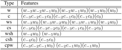
Type Features
w (w−3w−2w−1w0)(w−2w−1w0)(w−1w0)(w0)
c (c−3c−2c−1c0)(c−2c−1c0)(c−1c0)(c0)
ws (w−3w0)(w−3w−2w0)(w−3w−1w0)(w−2w0)
cs (c−3c0)(c−3c−2c0)(c−3c−1c0)(c−2c0)
wsh (w−4w0) (w−5w0)
csh (c−4c0) (c−5c0)
[image:7.595.309.524.62.151.2]cpw (c−3c−2c−1w0) (c−2c−1w0)(c−1w0)
Table 1: Feature definition in TDRF LMs
1999), denoted by KN4. We use the RNNLM toolkit5to train a RNNLM (Mikolov et al., 2011).
The number of hidden units is 250 and other configurations are set by default6.
Word classing has been shown to be useful in conditional ME models (Chen, 2009). For our TDRF models, we consider a variety of features as shown in Table 1, mainly based on word and class information. Each word is deterministically assigned to a single class, by running the automat-ic clustering algorithm proposed in (Martin et al., 1998) on the training data.
In Table 1,wi, ci, i= 0,−1, . . . ,−5denote the
word and its class at different position offset i, e.g. w0, c0 denotes the current word and its class.
We first introduce the classic word/class n-gram features (denoted by “w”/“c”) and the word/class skippingn-gram features (denoted by “ws”/“cs”) (Goodman, 2001a). Second, to demonstrate that long-span features can be naturally integrated in TDRFs, we introduce higher-order features “w-sh”/“csh”, by considering two words/classes sep-arated with longer distance. Third, as an example of supporting heterogenous features that combine different information, the crossing features “cp-w” (meaning class-predict-word) are introduced. Note that for all the feature types in Table 1, only the features observed in the training data are used. The joint SA (Algorithm 1) is used to train the TDRF models, with all the acceleration methods described in Section 4 applied. The minibatch size K = 300. The learning rates γλ and γζ
are configured as (29) and (19) respectively with βλ = βζ = 0.6 andtc = 3000. Fort0, it is first
initialized to be104. During iterations, we monitor
the smoothed log-likelihood (moving average of 1000 iterations) on the PTB development data.
5http://rnnlm.org/
6Minibatch size=10, learning rate=0.1, BPTT steps=5. 17
models PPL (±std. dev.)
KN4 142.72
RNN 128.81
[image:8.595.306.539.60.272.2]TDRF w+c 130.69±1.64
Table 2: The PPLs on the PTB test data. The class number is 200.
We sett0 to the current iteration number once the
rising percentage of the smoothed log-likelihoods within 100 iterations is below 20%, and then continue 5000 further iterations before stopping. The configuration of hessian estimation (Section 4.1) isγH =γλandh = 10−4. L2 regularization
with constant10−5is used to avoid over-fitting. 8
CPU cores are used to parallelize the algorithm, as described in Section 4.3, and the training of each TDRF model takes less than 20 hours.
The perplexity results on the PTB test data are given in Table 2. As the normalization constants of TDRF models are estimated stochastically, we report the Monte Carlo mean and standard devi-ation from the last 1000 iterdevi-ations for each PPL. The TDRF model using the basic “w+c” features performs close to the RNNLM in perplexity. To be compact, results with more features are presented in the following WSJ experiment.
5.2 WSJ speech recognition results
In this section, we continue to use the LMs ob-tained above (using PTB training and develop-ment data), and evaluate their performance mea-sured by WERs in speech recognition, by re-scoring 1000-best lists from WSJ’92 test data (330 sentences). The oracle WER of the 1000-best lists is 3.4%, which are generated from using the Kaldi toolkit7with a DNN-based acoustic model.
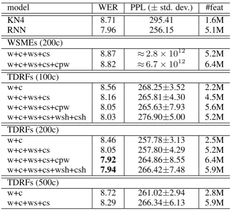
TDRF LMs using a variety of features and different number of classes are tested. The results are shown in Table 3. Different types of features, like the skipping features, the higher-order fea-tures and the crossing feafea-tures can all be easily supported in TDRF LMs, and the performance is improved to varying degrees. Particularly, the TDRF using the “w+c+ws+cs+cpw” features with class number 200 performs comparable to the RNNLM in both perplexity and WER. Numerical-ly, the relative reduction is 9.1% compared with the KN4 LMs, and 0.5% compared with the RNN LM.
7http://kaldi.sourceforge.net/
model WER PPL (±std. dev.) #feat
KN4 8.71 295.41 1.6M
RNN 7.96 256.15 5.1M
WSMEs (200c)
w+c+ws+cs 8.87 ≈2.8×10¹² 5.2M
w+c+ws+cs+cpw 8.82 ≈6.7×10¹² 6.4M
TDRFs (100c)
w+c 8.56 268.25±3.52 2.2M
w+c+ws+cs 8.16 265.81±4.30 4.5M w+c+ws+cs+cpw 8.05 265.63±7.93 5.6M w+c+ws+cs+wsh+csh 8.03 276.90±5.00 5.2M TDRFs (200c)
w+c 8.46 257.78±3.13 2.5M
w+c+ws+cs 8.05 257.80±4.29 5.2M w+c+ws+cs+cpw 7.92 264.86±8.55 6.4M w+c+ws+cs+wsh+csh 7.94 266.42±7.48 5.9M TDRFs (500c)
w+c 8.72 261.02±2.94 2.8M
[image:8.595.105.258.62.123.2]w+c+ws+cs 8.29 266.34±6.13 5.9M
Table 3: The WERs and PPLs on the WSJ’92 test data. “#feat” denotes the feature number. Differ-ent TDRF models with class number 100/200/500 are reported (denoted by “100c”/“200c”/“500c”)
5.3 Comparison and discussion
TDRF vs WSME. For comparison, Table 3 also
presents the results from our implementation of the WSME model (3), using the same features as in Table 1. This WSME model is the same as in (Rosenfeld, 1997), but different from (Rosenfeld et al., 2001), which uses the traditional n-gram LM as the priori distributionp0.
For the WSME model (3), we can still use a SA training algorithm, similar to that developed in Section 3.2, to estimate the parametersλ. But in this case, there is no need to introduceζl, because
the normalizing constantsZl(λ) are canceled out
as seen from (7). Specifically, the learning rateγλ
and theL2regularization are configured the same
as in TDRF training. A fixed number of iterations witht0 = 5000is performed. The total iteration
number is10000, which is similar to the iteration number used in TDRF training.
In order to calculate perplexity, we need to estimate the global normalizing constantZ(λ) = Pm
l=1Zl(λ) for the WSME model. Similarly
as in (Tan, 2015), we apply the SA algorithm in Section 3.2 to estimate the log normalizing constants ζ, while fixing the parameters λ to be those already estimated from the WSME model and using uniform probabilitiesπl≡m−1.
−494 and −509 respectively. However, the W-ERs from using the trained WSME models in hypothesis re-ranking are not as poor as would be expected from their PPLs. This appears to indicate that the estimated WSME parameters are not so bad for relative ranking. Moreover, when the estimatedλandζ are substituted into our TDRF model (6) with the empirical length probabilities πl, the “corrected” average test log-likelihoods
per sentence for these two sets of parameters are improved to be−152and−119respectively. The average test log-likelihoods are both−96 for the two corresponding TDRF models in Table 3. This is some evidence for the model deficiency of the WSME distribution as defined in (3), and intro-ducing the empirical length probabilities gives a more reasonable model assumption.
TDRF vs conditional ME. After training, TDRF
models are computationally more efficient in com-puting sentence probability, simply summing up weights for the activated features in the sentence. The conditional ME models (Khudanpur and Wu, 2000; Roark et al., 2004) suffer from the expen-sive computation of local normalization factors. This computational bottleneck hinders their use in practice (Goodman, 2001b; Rosenfeld et al., 2001). Partly for this reason, although building conditional ME models with sophisticated features as in Table 1 is theoretically possible, such work has not been pursued so far.
TDRF vs RNN. The RNN models suffer from
the expensive softmax computation in the output layer8. Empirically in our experiments, the
aver-age time costs for re-ranking of the 1000-best list for a sentence are 0.16 sec vs 40 sec, based on TDRF and RNN respectively (no GPU used).
6 Related Work
While there has been extensive research on con-ditional LMs, there has been little work on the whole-sentence LMs, mainly in (Rosenfeld et al., 2001; Amaya and Bened´ı, 2001; Ruokolainen et al., 2010). Although the whole-sentence approach has potential benefits, the empirical results of pre-vious WSME models are not satisfactory, almost the same as traditional n-gram models. After incorporating lexical and syntactic information, a mere relative improvement of 1% and 0.4%
8This deficiency could be partly alleviated with
some speed-up methods, e.g. using word clustering (Mikolov, 2012) or noise contrastive estimation (Mnih and Kavukcuoglu, 2013).
respectively in perplexity and in WER is reported for the resulting WSEM (Rosenfeld et al., 2001). Subsequent studies of using WSEMs with gram-matical features, as in (Amaya and Bened´ı, 2001) and (Ruokolainen et al., 2010), report perplexity improvement above 10% but no WER improve-ment when using WSEMs alone.
Most RF modeling has been restricted to fixed-dimensional spaces 9. Despite recent progress,
fitting RFs of moderate or large dimensions re-mains to be challenging (Koller and Friedman, 2009; Mizrahi et al., 2013). In particular, the work of (Pietra et al., 1997) is inspiring to us, but the improved iterative scaling (IIS) method for parameter estimation and the Gibbs sampler are not suitable for even moderately sized models. Our TDRF model, together with the joint SA al-gorithm and trans-dimensional mixture sampling, are brand new and lead to encouraging results for language modeling.
7 Conclusion
In summary, we have made the following contri-butions, which enable us to successfully train T-DRF models and obtain encouraging performance improvement.
• The new TDRF model and the joint SA train-ing algorithm, which simultaneously updates the model parameters and normalizing con-stants while using trans-dimensional mixture sampling.
• Several additional innovations including ac-celerating SA iterations by using Hessian information, introducing word classing to ac-celerate the sampling operation and improve the smoothing behavior of the models, and parallelization of sampling.
In this work, we mainly explore the use of fea-tures based on word and class information. Future work with other knowledge sources and larger-scale experiments is needed to fully exploit the advantage of TDRFs to integrate richer features.
8 Acknowledgments
This work is supported by Toshiba Corporation, National Natural Science Foundation of China (NSFC) via grant 61473168, and Tsinghua Ini-tiative. We thank the anonymous reviewers for helpful comments on this paper.
9Using local fixed-dimensional RFs in sequential models
References
Fredy Amaya and Jos´e Miguel Bened´ı. 2001. Im-provement of a whole sentence maximum entropy language model using grammatical features. In
Association for Computational Linguistics (ACL).
Albert Benveniste, Michel M´etivier, and Pierre Priouret. 1990. Adaptive algorithms and stochastic
approximations. New York: Springer.
Olivier Bousquet and Leon Bottou. 2008. The tradeoffs of large scale learning. In NIPS, pages 161–168.
Richard H Byrd, SL Hansen, Jorge Nocedal, and Yoram Singer. 2014. A stochastic quasi-newton method for large-scale optimization. arXiv preprint
arXiv:1401.7020.
Stanley F. Chen and Joshua Goodman. 1999. An em-pirical study of smoothing techniques for language modeling. Computer Speech & Language, 13:359– 394.
Hanfu Chen. 2002. Stochastic approximation and its
applications. Springer Science & Business Media.
Stanley F. Chen. 2009. Shrinking exponential lan-guage models. InProc. of Human Language Tech-nologies: The 2009 Annual Conference of the North American Chapter of the Association for
Computa-tional Linguistics.
Joshua Goodman. 2001a. A bit of progress in language modeling. Computer Speech & Language, 15:403– 434.
Joshua Goodman. 2001b. Classes for fast maximum entropy training. In Proc. of International Confer-ence on Acoustics, Speech, and Signal Processing
(ICASSP).
Peter J. Green. 1995. Reversible jump markov chain monte carlo computation and bayesian model determination.Biometrika, 82:711–732.
Ming Gao Gu and Hong-Tu Zhu. 2001. Maxi-mum likelihood estimation for spatial models by markov chain monte carlo stochastic approximation.
Journal of the Royal Statistical Society: Series B
(Statistical Methodology), 63:339–355.
Sanjeev Khudanpur and Jun Wu. 2000. Maximum en-tropy techniques for exploiting syntactic, semantic and collocational dependencies in language
model-ing. Computer Speech & Language, 14:355–372.
Daphne Koller and Nir Friedman. 2009. Probabilistic
graphical models: principles and techniques. MIT
press.
Faming Liang, Chuanhai Liu, and Raymond J Carroll. 2007. Stochastic approximation in monte carlo computation. Journal of the American Statistical
Association, 102(477):305–320.
Sven Martin, J¨org Liermann, and Hermann Ney. 1998. Algorithms for bigram and trigram word clustering.
Speech Communication, 24:19–37.
Tomas Mikolov, Stefan Kombrink, Lukas Burget, Jan H Cernocky, and Sanjeev Khudanpur. 2011. Extensions of recurrent neural network language model. In Proc. of International Conference on
Acoustics, Speech and Signal Processing (ICASSP).
Tom´aˇs Mikolov. 2012. Statistical language models based on neural networks. Ph.D. thesis, Brno
University of Technology.
Yariv Dror Mizrahi, Misha Denil, and Nando de Fre-itas. 2013. Linear and parallel learning of markov random fields.arXiv preprint arXiv:1308.6342. Andriy Mnih and Koray Kavukcuoglu. 2013. Learning
word embeddings efficiently with noise-contrastive estimation. InNeural Information Processing
Sys-tems (NIPS).
Stephen Della Pietra, Vincent Della Pietra, and John Lafferty. 1997. Inducing features of random fields.
IEEE Transactions on Pattern Analysis and Machine
Intelligence, 19:380–393.
Brian Roark, Murat Saraclar, Michael Collins, and Mark Johnson. 2004. Discriminative language modeling with conditional random fields and the perceptron algorithm. In Proceedings of the 42nd Annual Meeting on Association for Computational
Linguistics (ACL), page 47.
Ronald Rosenfeld, Stanley F. Chen, and Xiaojin Zhu. 2001. Whole-sentence exponential language mod-els: a vehicle for linguistic-statistical integration.
Computer Speech & Language, 15:55–73.
Ronald Rosenfeld. 1997. A whole sentence maximum entropy language model. In Proc. of Automatic
Speech Recognition and Understanding (ASRU).
Teemu Ruokolainen, Tanel Alum¨ae, and Marcus Do-brinkat. 2010. Using dependency grammar features in whole sentence maximum entropy language mod-el for speech recognition. InBaltic HLT.
Holger Schwenk. 2007. Continuous space language models. Computer Speech & Language, 21:492– 518.
Ilya Sutskever and Geoffrey E Hinton. 2007. Learn-ing multilevel distributed representations for high-dimensional sequences. In International Confer-ence on Artificial IntelligConfer-ence and Statistics
(AIS-TATS).
Zhiqiang Tan. 2015. Optimally adjusted mixture sam-pling and locally weighted histogram. InTechnical Report, Department of Statistics, Rutgers University.
Laurent Younes. 1989. Parametric inference for imperfectly observed gibbsian fields. Probability