Munich Personal RePEc Archive
A Comparative Study of GARCH and
EVT Model in Modeling Value-at-Risk
Li, Longqing
Suffolk University, Christopher Newport University
25 February 2017
Online at
https://mpra.ub.uni-muenchen.de/85645/
A Comparative Study of GARCH and EVT Model in Modeling Value-at-Risk
Longqing Li
Suffolk University
The paper addresses an inefficiency of the traditional approach in modeling the tail risk, particularly the day ahead forecast of Value-at-Risk (VaR), using Extreme Value Theory (EVT) and GARCH model. Specifically, I apply both models onto major countries stock markets daily loss, including U.S., U.K., China and Hong Kong between 2006 and 2015, and compare the relative forecasting performance. The paper differs from other studies in two important ways. First, it incorporates an asymmetric shock of volatility in the financial time series. Second, it applies a skewed fat-tailed return distribution using the Generalized Error Distribution (GED). The back-testing result shows that, on one hand, the conditional EVT performs equally well relative to GARCH model under the Generalized Error Distribution. On the other hand, the Exponential GARCH based model is the best performing one in Value-at-Risk forecasting, because it not only correctly identifies the future extreme loss, but more importantly, its occurrence is independent.
INTRODUCTION
Effective financial risk management is under the spotlight following the global financial crisis of 2008. One of the most popular tools in risk management is the Value-at-Risk (VaR), endorsed under the Basel Accord with the intent of internal control. It is defined as the upper quantile of a loss distribution under a given confidence level over a certain time horizon. In other words, it measures the extent of loss that financial firms could incur under a certain probability, and might arise if there is a severe economic recession, stock market crash or other event that triggers downside risk. For example, if the one month 5% Value-at-Risk is $100 million, it means there is a 5% chance the investment firm could lose more than $100 in any given month. Different goals set different confidence levels and time horizons. In internal risk control field, the standard practice is to use a confidence level of 95% over a one-day holding period.
one tail is thicker than the other. Therefore it is inappropriate to assume the Normal distribution of asset return in risk management, because it ignores the inherent attributes of financial returns.
As a result, a number of novel tools have been developed, like a non-parametric historical simulation (HS), a fully parametric approach such as GARCH (Generalized Autoregressive Conditional Heteroskedasticity), and Extreme Value Theory (EVT). The merit of historical simulation (HS) is that it makes no strict assumption about the distribution of assets, but it does assume a time-invariant distribution of returns. The standard GARCH model enables risk managers to take time-varying volatility into account in the financial market, though volatility responds in the same magnitude to both positive and negative shocks. And a number of studies show the superiority of EVT against classical models in modeling Value-at-Risk (Longin 2000; Bali 2007). In particular, the conditional EVT, a two-stage approach that integrates standard GARCH into EVT, is shown to be the best performing model in forecasting Value-at-Risk.
The increasing popularity of standard GARCH and EVT model has led us to think whether we could extend the existing models to better reflect the properties of financial market distributions, as well as to test the robustness of a conditional EVT model. The goal of the paper is to understand the comparative strengths and limits of both models in measuring Value-at-Risk under a less restrictive but more realistic environment. The paper is different from the existing literature in the following ways. First, it incorporates the asymmetric volatility in financial time series, the so-called leverage effect, to address the fact that volatility increases more on bad news than on good news. In other words, the standard GARCH model assumes volatility responds in the same way to positive or negative shock. Second, it uses a less restrictive but more flexible Generalized Error Distribution (GED) (Theodossiou 2015) to accommodate the fat tails and skewness exhibited in the distribution of return.
Since the financial institution usually holds a number of different assets like bonds, stocks, options, and futures in a portfolio, and frequently updates the composition on a daily basis, it is complicated to measure the real portfolio. Here I only focus on the stock market return in major developed and developing countries, including S&P500-US, FTSE100-UK, NASDAQ Composite-US, Hang Seng-Hong Kong and CSI300-China. The time period spans from early 2006 to late 2015, which encompasses the outbreak of global financial crisis in 2008, and the recent economic slowdown in China (biggest stock market crash in eight years). To assess the performance of Value-at-Risk estimation, I perform a dynamic backtesting procedure.
The remainder of the paper is structured as follows. Section 2 discusses the existing literature. Section 3 presents an overview of the GARCH family and EVT models, and shows the basic calculation of Value-at-Risk with conditional EVT and GARCH models. Section 4 describes the stock indexes used in the paper. Section 5 displays stylized facts, fitted performance, and empirical results. Section 6 introduces the backtesting and presents the test result. Section 7 concludes the study.
LITERATURE REVIEW
The prevailing parametric approach is to use a GARCH-type model to capture time-varying volatility of the distribution. Typical models include GARCH-normal, GARCH-t and GARCH-skewed t. The GARCH-normal model meets with harsh criticism because of its tendency to under-predict future risk. This leads to an adoption of the GARCH-t model to accommodate fat-tailed distribution. Lin and Shen (2006) find that the Student-t distribution moderately improves market risk estimation. But the Student-t distribution is symmetric, unable to reflect the asymmetric property of distribution of returns. Giotand Lauren (2003) show that a model with a symmetric probability density function underperforms relative to one with a skewed density function.
risk management and how it could be specifically embedded in estimating Value-at-Risk. Gilli and Këllezi (2006) apply EVT to the stock market indices to derive Value-at-Risk and corresponding confidence levels. Bali (2007) finds the EVT yields better performance with respect to skewed t and normal distributions using daily index of the Dow Jones Industrial Average (DJIA).
Although EVT is generally superior to Historical Simulation (HS), GARCH-normal, GARCH-t and GARCH-skewed t models, it has two main inherent disadvantages. First, in the short term, the risk manager is sometimes more interested in the loss over the next couple of days, in which case the EVT is unable to reflect time varying volatility. Second, it depends on the assumption of the distributions that are independent and identically distributed (iid), a strong hypothesis in financial time series.
Therefore it is reasonable to use the conditional EVT, also called GARCH-EVT. McNeil and Frey (2000) develop a two-stage procedure to estimate this, and show it is better suited for measuring the market risk. In the first stage, the distribution is estimated with a GARCH model to obtain identically and independent distributed (iid) residuals. In the second stage, standardized residuals are fitted using the EVT framework. In doing so, the conditional EVT could integrate time-varying volatility and tail risk simultaneously. Allen et al. (2013) find the conditional EVT-based approach produces the least amount of violations, defined as the actual loss greater than expected, in out-of-sample backtesting using FTSE100 and S&P500 index. Karmakar and Shukla (2015) further demonstrate conditional EVT to be the best-performing model in estimating Value-at-Risk of daily stock price indices in six different countries. Bali and Neftci (2003) find conditional EVT gives a more accurate measure of Value-at-Risk compared with a GARCH-skewed using U.S. short-term interest rates.
METHOD AND MODELING
Background of Value-at-Risk Models
As a common standard in risk management, Value-at-Risk is often defined as the quantile of return (loss) distribution of an asset. It measures how much loss could be realized in a worst-case scenario. From a risk managers perspective, it is more meaningful to hedge against the loss instead of the return, so the paper will focus on the loss distribution1 of an asset. Thus the upper tail of the loss distribution is considered as the Value-at-Risk. Here we define the difference in the daily logarithm of the stock price index as the return on the asset. Formally, let be the daily negative returns at time t. So the Value-at-Risk ( ) is the (1- ) quantile of the loss distribution at time t over a one-day horizon. With a (1- ) confidence level, the probability of loss exceeding than the threshold is less than . In mathematical form, it is Pr . So the Value-at-Risk calculation is based on the following equation
(1)
where F-1 is the quantile function, that is, the inverse of distribution function F and the conditional standard deviation at time t.
AR (1)-GARCH (1,1) Model
A natural generalization of the ARCH (Autoregressive Conditional Heteroskedasticity) model proposed by Engle (1982), which allows the conditional variance to change over time as a function of past errors, has proved to be a powerful tool in dealing with time-varying volatility, as volatility clustering is quite common in financial markets. The dynamics of the conditional mean of daily negative logarithm returns follows an AR (1) process,
where rt-1 is the lagged negative return and is the innovation term following generalized error distribution (GED).In what follows, we use the parsimonious AR (1)-GARCH (1,1) model. To be consistent with our naming conventions, we follow Bollerslevs (1986) guideline on each parameter.
Standard GARCH Model
The dynamics of the conditional variance equation are characterized by
(3)
where is the conditional variance of innovation term , is the intercept and + <1 to ensure stationarity of loss series. The standard GARCH model has proved to be useful in tackling volatility clustering, but it also highlights neither negative or positive shock should have any impact on the future volatility because the is dependent on the past squared residuals rather than itself. However a number of empirical studies have observed that a negative shock, like a market crash or economic crisis, triggers greater volatility relative to a positive shock such as economic growth. This brings us to the next model.
Exponential GARCH Model
To address the occurrence of an asymmetric effect in financial time series, Nelson (1991) proposes the EGARCH model, where the conditional variance is expressed as
(4)
Let be the standardized residual with mean 0 and constant variance; then it can be written as
(5)
where captures the leverage effect of a negative (positive) shock. If the past shock is positive, the impact on conditional volatility is while a negative past shocks effect on volatility equals
. We expect the leverage effect parameter to be negative.
Threshold GARCH Model
In the same way, the threshold GARCH (TGARCH) model, aka GJR model (Glosten et al 1993), examines the leverage effect based on the state of past innovation. Specifically, the conditional variance is determined by the threshold level 0, on whether the shock is positive or negative.
(6)
where
If the past innovation was positive, then the conditional variance is , while the effect of a negative innovation on volatility is . Hence a negative shock gives rise to greater volatility because >0.
Forecasting of GARCH Model
The one-step ahead forecast of conditional variance for standard GARCH, EGARCH and TGARCH model is
(8) (9) In the case of the GARCH model, the estimation of Value-at-Risk is
(10) where is the quantile of the generalized error distribution.
Extreme Value Theory
Rather than considering the whole sample in loss distribution, EVT only focuses on the tail behavior of the loss. In other words, it deals with the asymptotic limiting distribution of extreme value (large losses). In general, there are two fundamental approaches in modeling the extreme value. One is the block maximum (BM) [see Gumbell (1958)] that considers the largest value in each consecutive block as the extreme value. But the block maxima approach decreases the efficiency if other data on extreme values are available. The second is the peak over threshold (POT) approach in which we define the extreme as the observations exceeding a particular threshold. The probability distribution of the observations above the threshold follows a generalized Pareto distribution [see Pickands (1975)]. There are two major advantages of POT approach: First, it does not suffer from a lack of observations. Second, it offers a fully parametric approach that is easy to calculate and extrapolate. The paper follows the POT approach.
POT Model
Define the excess distribution above the threshold u as the conditional probability. Given a high threshold u, the probability distribution of excess value of X over the threshold is defined by
(11) Because of for X>u,
The purpose of above function is to construct a tail estimator. Balkema (1974) and Pickands (1975) argue that the limiting distribution of the excess could be approximated by the generalized Pareto distribution (GPD) given a sufficiently high threshold. The functional form of GPD is
(12)
where is the shape parameter and the scale parameter .
The above function embodies three type of distribution. If >0, it corresponds to the ordinary Pareto distribution. When =0, it is an exponential distribution. If <0, it is known as a Pareto type II distribution.
EVT and Estimation of Value-at-Risk
Here we follow McNeil and Freys (2000) method for determining the threshold2. We define N as the number of total observations, and n as the number of exceedances (values above the threshold u). If the threshold u is sufficiently large to balance the bias and variance, and each observation is independently and identically distributed (iid), then the exceedance follows the generalized Pareto distribution (GPD). Hence, the shape and scale parameters can be estimated with a maximum likelihood method (Smith, 1987). Thus the tail estimator is
(13)
If we invert3 the equation above, then the unconditional Value-at-Risk quantile with a given probability is
(14)
Despite the growing use of EVT in Value-at-Risk estimation, the assumption that observations are identically and independent distributed (iid) does not sit well with the reality of financial series data. The immediate solution is to use filtered data, the conditional EVT. That is, we fit a time-varying volatility model to the data, then estimate the tails of the standardized residuals retrieved from the fitted model using EVT. The advantage of conditional EVT is that it not only captures volatility clustering within the GARCH framework, but also explores the tail behavior with an EVT scheme simultaneously. The conditional EVT is described as follows:
1) The AR (1)-GARCH (1,1) model is fitted to the negative logarithm of returns using quasi-maximum likelihood estimation. Then we get a one step ahead forecast of conditional mean and conditional standard deviation .
2) Apply EVT to the standardized residual retrieved from Step 1 to get the estimate . The Value-at-Risk derived from conditional EVT can be expressed as:
where the unconditional
If we substitute with , then the GARCH-EVT based Value-at-Risk is
DATA DESCRIPTION
The recent shift in China from investment-led growth to a more-sustainable consumer-based growth model, accompanied with heavy-handed government interference in the stock market, makes it pressing to develop an effective risk-hedging strategy for the highly unstable market. The CSI300 index, a free-float weighted index that consists of 300 A-share stocks listed in the Shanghai and Shenzhen Stock Exchanges, has been considered as an important indicator of Chinese financial market. The inclusion could help us better gauge the market risk of Chinese stock market returns. To account for the outbreak of the global financial crisis, we further look at the most advanced financial markets in the U.S., U.K., Japan and Hong Kong. Each regions stock market plays a substantial role both at home and abroad.
accounted for. We compute the daily negative logarithm returns as , where price index at time t. The loss is considered as the negative logarithm return, thus the upper tail of the loss distribution is the Value-at-Risk. The in-sample period for the purpose of estimation is from 01/01/2006 to 04/03/2008 and out-of-sample period reserved for backtesting is between 04/04/2008 and 11/30/2015. Altogether we have 2204 observations of adjusted price index.
EMPIRICAL RESULT
Figure 1 shows both the daily stock index (left panel) and negative daily logarithm returns (right panel) for each market from the beginning of 2006 to the late 2015.The left panel suggests financial market in each country, for the most part, tends to move in the same direction simultaneously except China. As depicted from the figure, the 2008 global financial crisis caused the biggest drop, with stock market reaching historically the lowest level. The right panel points out the daily return of Chinese stock market moves up and down more rapidly than that of developed countries, underscoring the high volatility of developing countrys financial market.
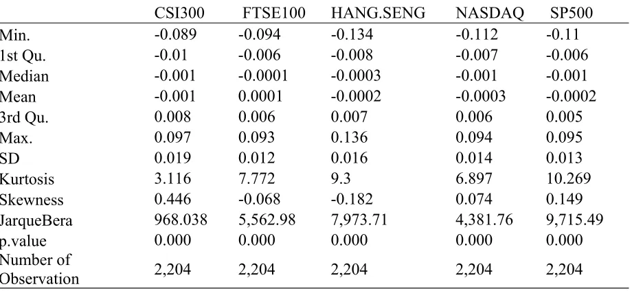
Table 1 reports the summary statistics of daily negative returns of stock market index. The negative mean loss indicates an overall upward movement of the stock index. Besides, we find that FTSE100 and Hang Seng experiences more frequent negative shock because of the negative skewness, while CSI300, NASDAQ and S&P500 endures more positive shock for the most of the time. The high excess kurtosis across all financial markets corroborates the fat tails in return (loss) distribution. Put differently, the extreme events particularly the significant loss, are much more likely to happen than we anticipate. To validate the normality of loss distribution, we perform the JarqueBera test. A greater test statistic gives a strong evidence of non-normality, which therefore indicates the estimation of Value-at-Risk with normal distribution is inappropriate and likely to underestimate the real risk.
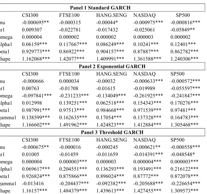
Table 2 presents the estimated parameters in mean and variance equation of three AR (1)-GARCH (1,1) models in negative daily logarithm returns. In the mean equation, and is the constant term and AR (1) coefficient respectively. All three models consistently show long-term average (the constant) close to zero and the loss negatively correlated with lagged terms. The variance equation demonstrates the high persistence ( ) of past squared residuals on current volatility, which manifests the volatility clustering in financial markets. In EGARCH and TGARCH panel, the parameter measures the leverage effect. In particular, the positive in EGARCH model reveals the conditional volatility is more sensitive to positive shock. Likewise, the negative in TGARCH paints a similar picture. In other words, both models support the positive shock exerts more influence on volatility, partly because of continually upward movement in stock index after global financial crisis.
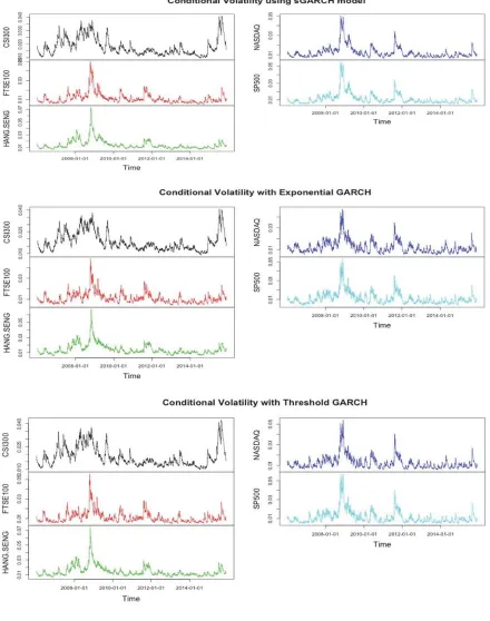
Figure 2 depicts the conditional volatility derived from three GARCH (1,1) models, respectively. As a whole, there is no significant discernable difference among all three models, all of which portray the similar picture of the volatility over time. The peak of the volatility resembles the global financial crisis in 2008. Except for CSI300 (China), the volatility declines gradually in post financial crisis. Interestingly enough for Chinese stock market, its trajectory is bumpy and far from smooth. The volatility of CSI300 rises and falls more substantially during the financial crisis, underscoring the greater uncertainty and instability in Chinese stock market. Such empirical finding provides further evidence of higher risk in investing Chinese market.
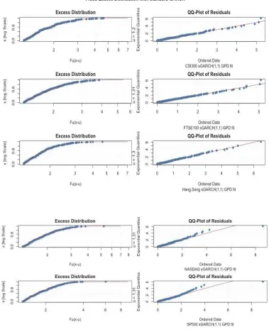
distribution of exceedance. Table 3 displays the estimate of static Value-at-Risk under a series of confidence level with different GARCH models. In all cases, the GARCH based estimate is greater than the normal one. Within each GARCH model, we find standard GARCH model, as a whole, yields a slightly higher estimate relative to EGARCH and TGARCH. On the other hand, there is not a substantial difference of the estimate between EGARCH and TGARCH. Also, a smaller estimate produced from normal distribution confirms its tendency to underestimate future downside risk.
DYNAMIC BACKTESTING
Value-at-Risk Model Evaluation
So far we have presented AR (1)-GARCH (1,1) based approach with three variations in calculating Value-at-Risk. In risk modeling, the ability to accurately predict future loss rather than overshooting or undershooting is the key in financial risk management. To evaluate the relative performance between GARCH and conditional EVT approach, we employ dynamic backtesting for the out-of-sample negative logarithm returns. Here we apply two types of backtesting criterions, unconditional coverage test (Kupiec 1995) and conditional coverage test (Christoffersen 1998).
Unconditional and Conditional Coverage Test
Let be a sequence of Value-at-Risk violations that can be described as:
then represents the number of days actual loss greater than the estimated Value-at-Risk over a T period. As seen from the equation above, the number of failure (loss greater than Value-at-Risk) follows a binomial distribution with the following likelihood ratio statistic:
(15)
Under the null hypothesis, the fraction of violation should be equal to the expected failure rate ( , is the confidence level for Value-at-Risk). Since this is a two-sided test, the model could be rejected because of either excessive or limited violations. The correct model (H0) is the one that produces reasonably right number of violations. The unconditional coverage test is straightforward to implement because it does not consider the dependence between the violations, that is, the timing of occurrence.
By standard, a good model requires not only an accurate prediction of the amount of violations over a length of time, but more importantly, the occurrence of violations should spread evenly. In other words, the violation is independent of each other, no violation clustering. Often the occurrence of violation clustering fails to detect the change in the market volatility. To that regard, we also use a more comprehensive procedure, proposed by Christoffersen (1998), called conditional coverage test. It jointly tests if the total number of violation equal to the expected one and the violation of Value-at-Risk independent over time. The test statistic of conditional coverage test is:
(16)
Under the null hypothesis, the occurrence of violation should be independent over time and the expected percentage of violation equals to . Given the model accurate, then violation today should not rely on the violation yesterday, which means and equals to each other.
Out-of-sample Dynamic Backtesting
For all stock market, we employ a rolling window of 1000 daily logarithm returns (4 years) to forecast one day ahead . In financial industry, the most commonly used procedure is to set at 5% particularly for internal risk control. Thus we conduct the dynamic backtesting at 5% level for all models, GARCH and conditional EVT. The advantage of rolling window procedure is twofold: to assess the stability of the model over time and the accuracy of the forecasting. Stability amounts to examining whether the coefficients time-invariant. In dealing with long period, it is not feasible to evaluate the fitted model everyday and to pick a new constant value of k (the number of days of exceedance over the threshold u) for tail estimation. Besides we set the 90 percentile of the loss distribution as the threshold (u), so k equals to 10% of daily observation.
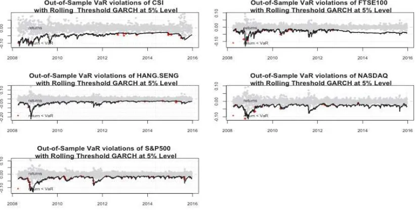
Conditional EVT means, on each day, we fit AR (1)-GARCH (1,1) model with three GARCH variations to each stock market and determine a new GPD tail estimate, computed from realized standardized residual. The violation ratio, the ratio between actual number of violations and total number of one-period forecast, is used to assess the performance of each model. A violation is realized if
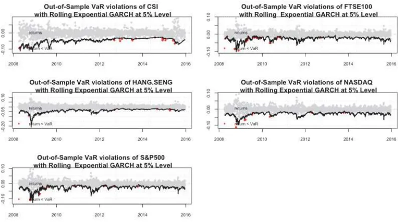
at time t+1. Define , then >1 refers to an underestimation of the realized loss since the actual violation is greater than the expected proportion. And <1 indicates an overestimation of future loss, consequently, setting aside unnecessary excessive amount of capital. In theory, a good model expects a violation ratio equal to , thus =1. With rolling window of 1000 observations, out-of-sample violation plot using GARCH model is presented in Figure 4,5,6. A red dot signals actual violation.
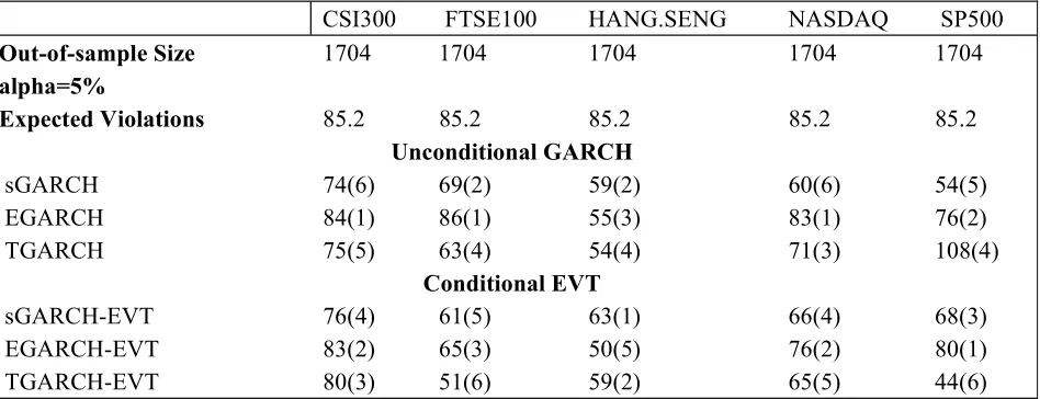
Table 4 presents the violation test result of all competing models. The ranking shows EGARCH-based model produces the best performance for all stock markets, except for Hang Seng, with 80% chance successfully passing the violation test. On the other hand, the TGARCH and standard GARCH model perform roughly equal well in predicting market risk, though both are less superior to EGARCH. Besides they both yield a smaller actual violation ratio relative to , meaning more likely to overestimate the actual loss, therefore increasing the cost in doing capital allocation. For instance, the expected number of violations, at 5% significance level, for each market is 85.25. And the standard GARCH model realizes an actual violation of 60 and 54 in NASDAQ and S&P500 market respectively, far away from the expected failure. The consequence of overshooting the risk is an uptick in unnecessary capital allocation, inflating the cost of doing business.
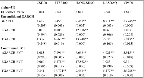
Table 5 is the unconditional coverage test of GARCH and conditional EVT model. Under the null hypothesis of correct exceedance, a good model should be the one that does not reject Ho. Hence the test with a higher p-value is an indication of appropriate model. For unconditional GARCH group, the EGARCH delivers a much greater p-value compared with the alternatives. Similarly, EGARCH-EVT yields a higher p-value in conditional EVT group. Both of these findings demonstrate the supremacy of EGARCH-based model.
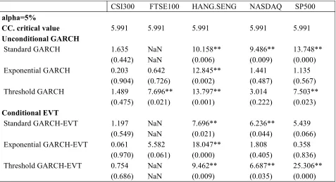
Table 6 is the conditional coverage test of two competing models. Likewise, a good model should accept the null hypothesis Ho, that is, correctly identifying the number of violations and being independent. The test result also indicates the EGARCH-based model stands out as the best one, achieving the highest success rate in violation test, as evidenced by a greater p-value.
CONCLUSION
Developing a statistically sound approach in estimating Value-at-Risk is critical in financial risk management. The inappropriateness of the ad hoc normal distribution and Student-t assumption in estimating Value-at-Risk has increased the popularity of the standard GARCH and extreme value theory model under a normal distribution of the return. And the studies find the conditional EVT, a mix of standard GARCH and EVT model, is the best performing tool in estimating Value-at-Risk. However standard GARCH model does not penalize the positive and negative shocks responding differently to the volatility. Nor the normal and Student-t distribution reflects the fundamental attributes of the financial assets. For that reason, I further investigate the existing findings by using a GARCH family model under a more comprehensive and less restricted distribution of the return, the generalized error distribution (GED). The backtesting result is different from other studies in a number of ways.
First, it does not find strong evidence pointing a complete superiority of extreme value theory (EVT). Instead, what is more superior is the exponential GARCH-based model, as supported by Angelidis (2004) claim that a combination of exponential GARCH and Student-t distribution gives the best estimate. Second, the dominance of conditional EVT is reduced when the return of distribution is controlled by the generalized error distribution. In other words, the conditional EVT and GARCH model performs equally well under the GED distribution. To conclude, the exponential GARCH-based model with GED is considered the best in modeling Value-at-Risk.
ENDNOTES
1. A loss distribution is the negative of a return distribution.
2. According to and Frey (2000), we choose 90th of the loss distribution as the threshold.
3. For details of the formula, see Embrechts, P., C. Klüppelberg, and T. Mikosch. 1997. Modeling Extremal Events.
4. For the sake of brevity, EGARCH and TGARCH diagnostic plot is not shown.
5. The expected failure is the product of a window size reserved for rolling estimation and a significant level; here it is 1704*0.05=85.2
6. The dataset covers from 01/01/2006 to 12/31/2015, here kurtosis represents the excess kurtosis (kurtosis less than 3) and the kurtosis of normal distribution is 3. A smaller p-value from Jarque-Bera test gives a strong evidence that the loss distribution is non-normal.
7. For each panel, the model is fitted with AR (1)-GARCH(1,1) .
8. The time series plot is from 01/01/2006 to 12/31/2015, the entire time period. 9. The daily time-varying volatility spans the entire time period, from 2006 to 2015.
10. For each figure, the in-sample period is from 01/01/2006 to 04/03/2008, and the out-of-sample period is from 04/04/2008 to 12/31/2015; a red dot represents an actual failure.
REFERENCES
Abad, P., S. Benito, and C. . (2014). A comprehensive review of Value-at-Risk methodologies. The Spanish Review of Financial Economics 12: 15--32.
Allen, D. E., A. K. Singh, and R. J. Powell. (2013). EVT and tail-risk modeling: Evidence from market indices and volatility series. The North American Journal of Economics and Finance 26: 355--369.
Alexios Ghalanos (2015). rugarch: Univariate GARCH models. R package version 1.3-6.
Angelidis, T., A. Benos, and S. Degiannakis. (2004). The use of GARCH models in Value-at-Risk estimation. Statistical Methodology 1:105128.
Bali T. G. (2007). A Generalized Extreme Value Approach to Financial Risk Measurement. J Money Credit Banking 39: 1613--1649.
Balkema, A. A., and L. de Haan. (1974). Residual Life Time at Great Age. Ann. Probability. 2:792804. Bekiros, S. D., and D. A. Georgoutsos. (2005). Estimation of Value-at-Risk by extreme value and
conventional methods: a comparative evaluation of their predictive performance. Journal of International Financial Markets, Institutions and Money 15: 209--28.
Bollerslev, T. (1986). Generalized autoregressive conditional heteroskedasticity. Journal of Econometrics
31:307327.
Christoffersen, P. F. (1998). Evaluating Interval Forecasts. International Economic Review 39:841. Dahlen, K. E., R. Huisman, and S. Westgaard. (2015). Risk Modeling of Energy Futures: A Comparison
of RiskMetrics, Historical Simulation, Filtered Historical Simulation, and Quantile Regression. Stochastic Models, Statistics and Their Applications: 283--291.
Danielsson, J .,& de Vries,C.(2000). Value-at-risk and extreme returns. Annales dEconomie et de Statistique,60, 239-270
Embrechts, P., C. Klüppelberg, and T. Mikosch. (1997). Modeling Extremal Events.
Embrechts, P., S. I. Resnick, and G. Samorodnitsky.(1999). Extreme Value Theory as a Risk Management Tool. North American Actuarial Journal 3:3041.
Engle, R. F. (1982). Autoregressive Conditional Heteroscedasticity with Estimates of the variance of United Kingdom Inflation. Econometrica 50:987.
Fernandez, V. (2005). Risk management under extreme events. International Review of Financial Analysis 14:113--148.
Gençay, R., F. Selçuk, and A. Ulugülya ci. (2003). High volatility, thick tails and extreme value theory in value-at-risk estimation. Insurance: Mathematics and Economics 33:337--356.
Gaye Gencer, H., and S. Demiralay. (2015). Volatility Modeling and Value-at-Risk (VaR) Forecasting of Emerging Stock Markets in the Presence of Long Memory, Asymmetry and Skewed Heavy Tails.
Emerging Markets Finance and Trade:1--19.
Ghorbel, A., and A. Trabelsi. (2008). Predictive performance of conditional Extreme Value Theory in Value-at-Risk estimation. International Journal of Monetary Economics and Finance 1:121. Gilli, M., and E.këllezi (2006). An Application of Extreme Value Theory for Measuring Financial Risk.
Computational Economics 27:207--228.
Giot, P., and S. Laurent. (2004). Modeling daily Value-at-Risk using realized volatility and ARCH type models. Journal of Empirical Finance 11:379--398.
Glantz, M., and R. Kissell. (2014). Extreme Value Theory and Application to Market Shocks for Stress Testing and Extreme Value-at-Risk. Multi-asset Risk Modeling:437--476.
Glosten, L. R., R. Jagannathan, and D. E. Runkle (1993). On the Relation between the Expected Value and the Volatility of the Nominal Excess Return on Stocks. The Journal of Finance 48:1779--1801.
Karmakar, M., and G. K. Shukla. (2015). Managing extreme risk in some major stock markets: An extreme value approach. International Review of Economics & Finance 35:1--25.
Kittiakarasakun, J., and Y. Tse. (2011). Modeling the fat tails in Asian stock markets. International Review of Economics & Finance 20:430--440.
Kuester, K. (2005). Value-at-Risk Prediction: A Comparison of Alternative Strategies. Journal of Financial Econometrics 4:53--89.
Kupiec, P. H. (1995). Techniques for Verifying the Accuracy of Risk Measurement Models. Derivatives
3:73--84.
Lieberman, G. J., and E. J. Gumbel. (1960). Statistics of Extremes. Journal of the American Statistical Association 55:383
Lin, C., and S. Shen. (2006). Can the Student-t distribution provide accurate Value-at-Risk? The Journal of Risk Finance 7:292--300.
Marimoutou, V., B. Raggad, and A. Trabelsi. (2009). Extreme Value Theory and Value-at-Risk: Application to oil market. Energy Economics 31:519--530.
McNeil, A. J., and R. Frey. (2000). Estimation of tail-related risk measures for heteroscedastic financial time series: an extreme value approach. Journal of Empirical Finance 7:271--300.
Nelson, D. B. (1991). Conditional Heteroskedasticity in Asset Returns: A New Approach. Econometrica
59:347.
Pickands, J.III, (1975). Statistical Inference Using Extreme Order Statistics. The Annals of Statistics
3:119131.
Poon, S.-H., and C. W. J. Granger. (2002). Forecasting Volatility in Financial Markets: A Review (revised edition). SSRN Journal.
Smith, R. L. (2002). Measuring Risk with Extreme Value Theory. Value-at-Risk and Beyond:224--246. Theodossiou, P. (2015). Skewed Generalized Error Distribution of Financial Assets and Option Pricing.
APPENDIX A, TABLES
[image:14.612.92.552.136.348.2]TABLE 1
SUMMARY STATISTICS OF DAILY LOSS FROM PRICE INDEX 6
CSI300
FTSE100 HANG.SENG
NASDAQ SP500
Min.
-0.089
-0.094
-0.134
-0.112
-0.11
1st Qu.
-0.01
-0.006
-0.008
-0.007
-0.006
Median
-0.001
-0.0001
-0.0003
-0.001
-0.001
Mean
-0.001
0.0001
-0.0002
-0.0003
-0.0002
3rd Qu.
0.008
0.006
0.007
0.006
0.005
Max.
0.097
0.093
0.136
0.094
0.095
SD
0.019
0.012
0.016
0.014
0.013
Kurtosis
3.116
7.772
9.3
6.897
10.269
Skewness
0.446
-0.068
-0.182
0.074
0.149
JarqueBera
968.038
5,562.98
7,973.71
4,381.76
9,715.49
p.value
0.000
0.000
0.000
0.000
0.000
Number of
TABLE 2
ESTIMATED PARAMETERS FROM GARCH FAMILY TYPE7
Panel 1 Standard GARCH
CSI300 FTSE100 HANG.SENG NASDAQ SP500 mu -0.000695** -0.000315 -0.00044* -0.000975*** -0.000816*** ar1 0.009307 -0.022781 -0.017432 -0.025061 -0.05849** omega 0.000004 0.000002 0.000002 0.000003 0.000002 alpha1 0.06159*** 0.117667*** 0.086249*** 0.10241*** 0.12401*** beta1 0.929773*** 0.86922*** 0.904157*** 0.87887*** 0.862782*** shape 1.162068*** 1.42077*** 1.409991*** 1.361588*** 1.240306***
Panel 2 Exponential GARCH
CSI300 FTSE100 HANG.SENG NASDAQ SP500 mu -0.000666 0.000034 -0.00032 -0.000633*** -0.000572*** ar1 0.00763 -0.01708 -0.01615 -0.019989 -0.055597*** omega -0.097841*** -0.231233*** -0.134049*** -0.261925*** -0.241847*** alpha1 0.012998 0.139251*** 0.062518*** 0.154343*** 0.170276*** beta1 0.987991*** 0.97513*** 0.984668*** 0.971539*** 0.97481*** gamma1 0.138599*** 0.162635*** 0.17054*** 0.137328*** 0.164783*** shape 1.166602*** 1.491962*** 1.424823*** 1.412884*** 1.305468***
Panel 3 Threshold GARCH
CSI300 FTSE100 HANG.SENG NASDAQ SP500 mu -0.000675** -0.000016 -0.000245 -0.000621** -0.000558*** ar1 0.01005 -0.01459 -0.011659 -0.014391*** -0.048548* omega 0.000004 0.000003*** 0.000003 0.000004*** 0.000003*** alpha1 0.069617*** 0.204551*** 0.136293*** 0.193491*** 0.216122*** beta1 0.926824*** 0.875866*** 0.896024*** 0.87772*** 0.872078*** gamma1 -0.013416 -0.204437*** -0.092382*** -0.205688*** -0.226654*** shape 1.16157*** 1.484379*** 1.439613*** 1.427455*** 1.309573***
TABLE 3
STATIC VALUE-AT-RISK FROM GARCH FAMILY TYPE
Prob Normal CSI300 FTSE100 HANG.SENG NASDAQ SP500
Panel A Static Value-at-Risk (VaR) from Standard GARCH (sGARCH)
0.95 1.645 1.7153 1.8102 1.7120 1.8373 1.8536 0.99 2.326 2.8348 2.7503 2.6116 2.8686 2.9703 0.995 2.576 3.2889 3.0757 2.9816 3.2455 3.3961
Panel B Static Value-at-Risk (VaR) from Exponential GARCH (EGARCH)
0.95 1.645 1.7181 1.7431 1.6999 1.8190 1.8351 0.99 2.326 2.8238 2.7570 2.5850 2.8295 2.9600 0.995 2.576 3.2697 3.1531 2.9383 3.2122 3.3991
Panel C Static Value-at-Risk (VaR) from Threshold GARCH (TGARCH)
0.95 1.645 1.7096 1.7577 1.7082 1.8229 1.8292 0.99 2.326 2.8278 2.7537 2.5736 2.8144 2.9336 0.995 2.576 3.2926 3.1195 2.9059 3.1810 3.3625
TABLE 4
OUT-OF-SAMPLE 1 DAY AHEAD VALUE-AT-RISK VIOLATION
CSI300 FTSE100 HANG.SENG NASDAQ SP500 Out-of-sample Size 1704 1704 1704 1704 1704
alpha=5%
Expected Violations 85.2 85.2 85.2 85.2 85.2 Unconditional GARCH
sGARCH 74(6) 69(2) 59(2) 60(6) 54(5) EGARCH 84(1) 86(1) 55(3) 83(1) 76(2) TGARCH 75(5) 63(4) 54(4) 71(3) 108(4)
Conditional EVT
sGARCH-EVT 76(4) 61(5) 63(1) 66(4) 68(3) EGARCH-EVT 83(2) 65(3) 50(5) 76(2) 80(1) TGARCH-EVT 80(3) 51(6) 59(2) 65(5) 44(6)
[image:16.612.87.561.404.586.2]TABLE 5
STATISTICAL TEST OF 1 DAY AHEAD UNCONDITIONAL COVERAGE (UC) TEST
CSI300 FTSE100 HANG.SENG NASDAQ SP500
alpha=5%
UC.critical value 3.841 3.841 3.841 3.841 3.841 Unconditional GARCH
sGARCH 1.619 3.458 9.461** 8.711** 13.748** (0.203) (0.063) (0.002) (0.003) (0.000) EGARCH 0.018 0.008 12.816** 0.060 1.083 (0.894) (0.929) (0.000) (0.806) (0.298) TGARCH 1.337 6.668** 13.748** 2.635 5.943** (0.248) (0.010) (0.000) (0.105) (0.015) Conditional EVT
sGARCH-EVT 1.083 7.996** 6.668** 4.921** 3.915** (0.298) (0.005) (0.010) (0.027) (0.048) EGARCH-EVT 0.060 5.471** 17.862** 1.083 0.341 (0.806) (0.019) (0.000) (0.298) (0.559) TGARCH-EVT 0.341 16.774** 9.461** 5.472** 25.288** (0.559) (0.000) (0.002) (0.019) (0.000)
Note: The table shows the statistics and p-value of unconditional coverage test of each competing model; p-value is represented in parentheses, ** denotes significant at 5% level
Unconditional coverage (UC) is chi-squared distributed with degrees of freedom of 1
TABLE 6
STATISTICAL TEST OF 1 DAY AHEAD CONDITIONAL COVERAGE (CC) TEST
CSI300 FTSE100 HANG.SENG NASDAQ SP500
alpha=5%
CC. critical value 5.991 5.991 5.991 5.991 5.991 Unconditional GARCH
Standard GARCH 1.635 NaN 10.158** 9.486** 13.748** (0.442) NaN (0.006) (0.009) (0.000) Exponential GARCH 0.203 0.642 12.845** 1.441 1.135 (0.904) (0.726) (0.002) (0.487) (0.567) Threshold GARCH 1.489 7.696** 13.797** 3.014 7.503** (0.475) (0.021) (0.001) (0.222) (0.023) Conditional EVT
Standard GARCH-EVT 1.197 NaN 7.696** 6.236** 5.439 (0.549) NaN (0.021) (0.044) (0.066) Exponential GARCH-EVT 0.061 5.582 18.047** 1.808 0.358 (0.970) (0.061) (0.000) (0.405) (0.836) Threshold GARCH-EVT 0.754 NaN 9.462** 6.687** 25.306** (0.686) NaN (0.009) (0.035) (0.000)
Note: The table shows the statistics and value of conditional coverage of each competing model; p-value is represented in parentheses, ** denotes significant at 5% level
Conditional coverage(CC) is chi-squared distributed with degrees of freedom of 2
APPENDIX B, FIGURES
[image:19.612.76.508.175.441.2]FIGURE 1
FIGURE 2
FIGURE 3
FIGURE 4
OUT-OF-SAMPLE DYNAMIC BACKTESTING FROM STANDARD GARCH10
FIGURE 5
FIGURE 6