Shape Factor Asymptotic Analysis I

Shape Factor Asymptotic Analysis I

Wang, Frank Xuyan

2019

Online at

https://mpra.ub.uni-muenchen.de/93357/

Xuyan Frank Wang [0000-0001-7653-5755]

Validus Research Inc., 187 King Street South Unit 201, Waterloo, Ontario, Canada N2J 1R1

[email protected]

Abstract. The shape factor defined as kurtosis divided by skewness squared 𝐾

𝑆2

is characterized as the only choice among all factors 𝐾

|𝑆|𝛼, 𝛼 > 0 which is greater

than or equal to 1 for all probability distributions. For a specific distribution fam-ily, there may exists α>2 such that min_|𝑆|𝐾𝛼≥ 1. The least upper bound of all such

α is defined as the distribution’s characteristic number. The useful extreme values of the shape factor for various distributions which are found numerically before, the Beta, Kumaraswamy, Weibull, and GB2 Distribution, are derived using as-ymptotic analysis. The match of the numerical and the analytical results can be considered prove of each other. The characteristic numbers of these distributions are also calculated. The study of the boundary value of the shape factor, or the shape factor asymptotic analysis, help reveal properties of the original shape fac-tor, and reveal relationship between distributions, such as between the Kumaras-wamy distribution and the Weibull distribution.

Keywords: Shape Factor, Skewness, Kurtosis, Asymptotic Expansion, Beta Distribution, Kumaraswamy Distribution, Weibull Distribution, GB2 Distribu-tion, Computer Algebra System, Numerical OptimizaDistribu-tion, Characteristic Num-ber.

1

Introduction

The concept of shape factor is proposed and studied for various probability distribution families [1][2] ([1] has more background and references, [2] is more cogent). Three kind of uses are made of the shape factor: the global lower bound of the shape factor for a distribution family can be used to eliminate those distributions for data fitting that have these bound higher than the data distribution; when these bounds are not violated, the plot of the minimum shape factor value for given parameter can be used to locate the allowable range of that parameter; combine the shape factor plot with skewness plot, for known sign of the skewness, the allowable parameters ranges can be identified. Since in practice we mostly see positive skewness, we will generally restrict our anal-ysis to the positive skewness region.

functions, or the allowable numerical range for machine-precision numbers and arbi-trary-precision numbers. The remedy for the system error is to check by software that are using different under-the-hood implementations. The operational or human error is occurred when manipulating the mathematical expressions, such as using not exactly equivalent substitutions or transformations. To reduce this kind of error, multiple ap-proaches need to undertake to validate each other. The numerical and graphical results need to be subsidized by analytical deductions.

When the minimum of the shape factor is attained at the region interior, it can be found from the zero point of the partial derivatives. This is an application of differential analysis and root finding. The other case is at the boundary, usually either at 0 or infin-ity, an application of limit and asymptotic expansion/analysis.

We will redo the mathematical analysis of the Beta, Kumaraswamy, GB2, GB1, and GH distributions shape factors, with either new formulas found, or more analytical ways to support our original empirical plots, adding more rigorousness to our conclu-sions. To avoid repetition, we will resort to [1] or [2] heavily for most of the omitted contents. The GB1, GH studies will be in a second paper due to page length limitation.

2

Results

2.1 Shape Factor Characterization

The shape factor is found and defined in Wang [1][2], where simple power and expo-nential forms of distributions examples are used to justify that definition. Here we find more reason for the uniqueness of this definition.

For a random variable 𝑓 with mean 𝑚_𝑓, the following characteristics are defined:

 Moment (M), 𝑀[𝑟] ≡ ∫ 𝑓𝑟𝑑𝜇, 𝑟 > 0,

 Central Moment (CM), 𝐶𝑀[𝑟] ≡ ∫(𝑓 − 𝑚_𝑓)𝑟𝑑𝜇, 𝑟 > 0,

 Absolute Central Moment (ACM), 𝐴𝐶𝑀[𝑟] ≡ ∫|𝑓 − 𝑚_𝑓|𝑟𝑑𝜇, 𝑟 > 0,

 Skewness (S), 𝑆 ≡ 𝐶𝑀[3]

𝐶𝑀[2]32,

 Kurtosis (K), 𝐾 ≡ 𝐶𝑀[4]

𝐶𝑀[2]2,

 Shape Factor (SF), 𝑆𝐹 ≡ 𝐾

𝑆2=𝐶𝑀[4]∗𝐶𝑀[2]_𝐶𝑀[3]2 ,

 _{𝑆𝐹3[𝑟] ≡} 𝐴𝐶𝑀[𝑟]

𝐴𝐶𝑀[1]𝑟≤ 1, 𝑤ℎ𝑒𝑟𝑒 0 < 𝑟 < 1 and 𝑆𝐹3[𝑠] ≡_{𝐴𝐶𝑀[1]}𝐴𝐶𝑀[𝑠]𝑠≥ 1, 𝑤ℎ𝑒𝑟𝑒 𝑠 > 1,

 Standard Deviation (SD), 𝑆𝐷 ≡ 𝐴𝐶𝑀[2]12,

 Absolute Mean Deviation (MD), 𝑀𝐷 ≡ 𝐴𝐶𝑀[1],

 𝑆𝐹3[2] = (_𝑀𝐷𝑆𝐷)2_.

By Jensen’s inequality (https://en.wikipedia.org/wiki/Jensen's_inequality) we have:

(

∫(

)

From [1], we also know that 𝐾 ≥ 𝑆2, 𝐾 ≥ 𝑆2≥ |𝑆| 𝑖𝑓 |𝑆| ≥ 1, 𝐾 ≥ 1 > |𝑆| 𝑖𝑓 |𝑆| <

1. So we arrive at the following:

𝐾 ≥ |𝑆|,_|𝑆|𝐾 ≥ 1. (2)

We can similarly get (by monotonicity of |𝑆|αw.r.t. α):

𝐾 ≥ 𝑆43,𝐾

𝑆43≥ 1, (3)

𝐾 ≥ |𝑆|α_, 𝐾

|𝑆|α≥ 1, 𝑖𝑓 0 ≤ α ≤ 2. (4)

The equation (2)-(4) can be used where the quotient can give simpler forms. For example, if the central moment have simpler forms than the skewness and kurtosis, then (3) will be simpler, involving only 𝐶𝑀[4]

𝐶𝑀[3]43.

Equation (4) says that the shape factor is among an extended family of shape factors

𝐾

|𝑆|α that are bound below by 1, so we will call all of them the shape factors.

We postulate that 2 is the least upper bound of all α such that 𝐾

|𝑆|α≥ 1 hold for all

distribution families (that is, the condition in equation (4) is not only sufficient, but also necessary). But for a specific distribution family this inequality may hold for α larger than 2. These statements will be proved by example cases in section 2.3.

We guess for each specific distribution family there exists a critical value of α which is not less than 2, such that above it the minimum of 𝐾

|𝑆|αwill be 0, and below it, the

minimum of 𝐾

|𝑆|αwill be bigger than 1. We will call such a critical value where the

min-imums of the shape factors have a sharp jump the critical value or the characteristic number of the distribution.

The limit of the extended shape factors at 0 or infinity for parameters usually has simpler form that can be considered as a prototype, asymptotic value, or magnitude of order [3], in some cases are also the lower or upper bound, of the shape factors. The properties of these simpler form will give hint of similar properties for the original shape factors, such as for the critical value we guessed. We will start that limit calcula-tion with the simplest distribucalcula-tion in the next seccalcula-tion.

2.2 Beta Distribution

With the naming and parameterization convention for probability distributions from Mathematica or [4], for the 𝐵𝑒𝑡𝑎𝐷𝑖𝑠𝑡𝑟𝑖𝑏𝑢𝑡𝑖𝑜𝑛[𝛼, 𝛽], we have

𝑆𝐹 =3(2+𝛼+𝛽)(𝛼(−2+𝛽)𝛽+2𝛽_{4(𝛼−𝛽)}2_{(3+𝛼+𝛽)}2+𝛼2(2+𝛽)). (5)

For a fixed β, the lower boundary value at α=0 is the minimum value of the shape factor:

limit_𝛼→0 𝑆𝐹 = 𝑚𝑖𝑛_0<𝛼<𝛽𝑆𝐹 =3(2+𝛽)_2(3+𝛽). (6)

This value increases from 1 to 1.5 when β turns from 0 to ∞.

For a fixed α, the upper boundary at β=∞ and the minimum value of the shape factor are different:

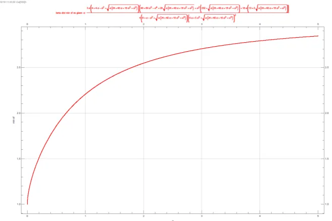
𝑚𝑖𝑛_𝛽>𝛼𝑆𝐹 = 3𝛼(4+4𝛼−𝛼2+√𝛼(24+40𝛼+16𝛼2+𝛼3))

4(6+𝛼−𝛼2_{+√𝛼(24+40𝛼+16𝛼}2_+𝛼3_{))(6𝛼+5𝛼}2_{+√𝛼(24+40𝛼+16𝛼}2_+𝛼3₎₎2(48 +

68𝛼3_{− 𝛼}4_{+ 28√𝛼(24 + 40𝛼 + 16𝛼}2_{+ 𝛼}3_{) + 𝛼}2_{(232 +}

√𝛼(24 + 40𝛼 + 16𝛼2_{+ 𝛼}3_{)) + 16𝛼 (13 + 2√𝛼(24 + 40𝛼 + 16𝛼}2_{+ 𝛼}3_{))), (7)}

𝑙𝑖𝑚𝑖𝑡_𝛽→∞ 𝑆𝐹 =3(2+𝛼)₄ . (8)

The upper boundary value of the shape factor for β=∞ increases from 1.5 to ∞ when

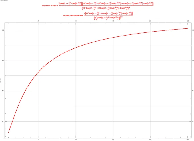
αturns from 0 to ∞. For given α, the minimum value of the shape factor increases from 1 to 3 when αturns from 0 to ∞, Fig. 1.

Fig. 1. Beta distribution minimum shape factor for given α in the horizontal axis.

limit

𝛽→∞ 𝑆 = 𝑚𝑎𝑥β>𝛼 𝑆 = 2

√𝛼, (9)

limit

𝛽→∞ 𝐾 = 𝑚𝑎𝑥β>𝛼 𝐾 = 3 + 6

𝛼. (10)

In practice, the equation (6) and (9) give relatively good (less than 10% error) upper bound estimate for the parameters β and α from data 𝑆𝐹 and 𝑆. This can be roughly stated as the skewness determines α, the higher the skewness the smaller the α, and the shape factor determines β, the higher the shape factor, the bigger the β. So in the Beta distribution case, the asymptotic analysis heuristically reveals the intrinsic meaning of

the parameters: α for skewness and β for shape factor.

2.3 Kumaraswamy Distribution Part One

Given Skewness

Even though more complex than Beta distribution, we will see that the limit and mini-mum value of the shape factor of the 𝐾𝑢𝑚𝑎𝑟𝑎𝑠𝑤𝑎𝑚𝑦𝐷𝑖𝑠𝑡𝑟𝑖𝑏𝑢𝑡𝑖𝑜𝑛[𝛼, 𝛽] show simi-lar pattern as the Beta distribution.

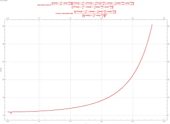
Fig. 2. Kumaraswamy distribution ratio of skewness contour tangent to kurtosis con-tour tangent plot.

Fig. 3. Kumaraswamy distribution maximum shape factor and log normal distribu-tion shape factor with respect to skewness plot.

Boundary α=0

For given β, when α→0, we will use the following 2nd _{order asymptotic expansion} at ∞ for 𝑥:

Beta[𝛽, 𝑥] → Gamma[𝛽]₂₄1 𝑥−2−𝛽_(24𝑥2_{− 12𝑥(−1 + 𝛽)𝛽 + 𝛽(2 − 3𝛽 − 2𝛽}2₊

3𝛽3_{)). (11)}

To find the asymptotic order of a function, we will utilize the following heuristic trick:

if 𝑑log (𝑓(𝑥))

𝑑𝑥 𝑥 → a, then possibly𝑓(𝑥)~𝑥a. (12)

The computer algebra system (CAS) Mathematica may be able to find the first limit when it cannot prove the second formula. Combining these techniques, we finally get:

limit

𝛼→0 {𝑆, 𝐾, 𝑆𝐹}~{

(2₃)𝛽 √2−𝛽₍1

𝛼)−𝛽𝛽Gamma[𝛽]

, (𝛼1)𝛽

𝛽Gamma[𝛽], ( 9

8)𝛽}. (13)

We see that skewness and kurtosis turn to infinity but the shape factor has finite limit. For a>0, from equation (13), we have:

limit_α→0 𝐾 limit_α→0 𝑆a~ (

1 𝛼)

(1−a₂)𝛽

From equation (14) we see that when a>2, limit

𝛼→0 𝐾

𝑆a~0; when 0<a<2, limit_{𝛼→0 𝑆}𝐾a~∞;

when a=2, limit

𝛼→0 𝐾

𝑆a~(9₈)𝛽. The Kumaraswamy distribution shows that the shape factor

with a=2 is the only definition that gives nonzero and finite boundary shape factor val-ues, and when a>2 this value is 0. This conclusion is also true for the Beta distribution by equation (9) and (10).

This observation is not limited to the Kumaraswamy or the Beta distribution, for example, but valid also for the following kind of distribution with power function prob-ability density function (PDF) 𝑛+1

𝑛 (1 − 𝑥𝑛), 𝑥 ∈ [0,1], 𝑛 > −1 , which is neither

Ku-maraswamy nor Beta distribution, it is also not GB1 as defined in [5], [6], or [4], having

𝑆 =

6√3(1 + 𝑛)(4 + 𝑛(3 + 𝑛)) (_{(1 + 𝑛)(7 + 𝑛(4 + 𝑛))}3 + 𝑛 )

3 2⁄

(3 + 𝑛)(4 + 𝑛) ,

𝐾 =

9(3 + 𝑛) (572 + 𝑛 (1011 + 𝑛 (813 + 𝑛 (366 + 𝑛(102 + 𝑛(15 + 𝑛))))))

5(1 + 𝑛)(4 + 𝑛)(5 + 𝑛)(7 + 𝑛(4 + 𝑛))2 , 𝑆𝐹 =(4+𝑛)(7+𝑛(4+𝑛))(572+𝑛(1011+𝑛(813+𝑛(366+𝑛(102+𝑛(15+𝑛))))))_{60(5+𝑛)(4+𝑛(3+𝑛))}2 . (15)

When n→-1, only SF (used a=2) converges to a nonzero finite number 1.2. So these three types of distributions all have characteristic number 2. These examples are proofs of our postulation in section 2.1.

2.4 Weibull Distribution

If not for power function, but for exponential function form of the PDF, such as the exponential distribution family [1] with PDF 𝑒−𝑥𝑛𝑛𝑥−1+𝑛, 𝑥 ∈ (0, ∞), 𝑛 > 0, which is

𝑊𝑒𝑖𝑏𝑢𝑙𝑙𝐷𝑖𝑠𝑡𝑟𝑖𝑏𝑢𝑡𝑖𝑜𝑛[𝑛, 1] or 𝐺𝑎𝑚𝑚𝑎𝐷𝑖𝑠𝑡𝑟𝑖𝑏𝑢𝑡𝑖𝑜𝑛[1,1, 𝑛, 0] or

𝑀𝑖𝑛𝑆𝑡𝑎𝑏𝑙𝑒𝐷𝑖𝑠𝑡𝑟𝑖𝑏𝑢𝑡𝑖𝑜𝑛[1,1_𝑛, −1_𝑛], will it behave similarly: the kurtosis divided by the squared skewness is the only choice which gives nonzero finite value when the skew-ness and kurtosis are infinite? Or will it have a critical value bigger than 2? We will see that it is the second case, and start the study from its central moment:

{𝐶𝑀[2], 𝐶𝑀[3], 𝐶𝑀[4]} = {−Gamma [1 +1_𝑛]2+ Gamma [1 +2_𝑛] , 2Gamma [1 +

1 𝑛]

3

− 3Gamma [1 +_𝑛1] Gamma [1 +_𝑛2] + Gamma [1 +3_𝑛] , −3Gamma [1 +1_𝑛]4+ 6Gamma [1 +_𝑛1]2Gamma [1 +2_𝑛] − 4Gamma [1 +_𝑛1] Gamma [1 +_𝑛3] +

Gamma [1 +4_𝑛]}. (16)

Algebraic or more quickly numerical method can be used to find inequalities or to com-pare orders. For example, we can deduct either by 𝐶𝑀[2] ≥ 0 or from the numerical minimum NMinimize [{−Gamma [_𝑛1]2+ 2𝑛Gamma [2_𝑛] , 𝑛 > 0} , {𝑛, 1 10⁄ , 1000}] =

{0.8425644753494974, {𝑛 → 1.6219726504389582}} that:

2𝑛Gamma [2_𝑛] > Gamma [1_𝑛]2, 𝑤ℎ𝑒𝑛 𝑛 > 0. (17)

This inequality is unique of the Gamma function, and is not hold for general log convex functions. It gives us idea or hint of the dominance of terms, then either by plot

or by calculating symbolic limit of Gamma[

1 𝑛]2

2𝑛Gamma[2_𝑛] we know the squared term in 𝐶𝑀[2] can

be ignored.

We finally get the asymptotic expansion of (16) when n→0 from those

simplifica-tions and other simplificasimplifica-tions such as using the formula (a + 𝑛)a𝑛→ 𝑒aa𝑛, where we cannot simply remove the 𝑛 in the sum without add the factor 𝑒 in:

limit

𝑛→0 {𝐶𝑀[2], 𝐶𝑀[3], 𝐶𝑀[4]}~{( 2 ⅇ𝑛)

2 𝑛√4𝜋

𝑛, ( 3 ⅇ𝑛)

3 𝑛√6𝜋

𝑛, ( 4 ⅇ𝑛)

4 𝑛√8𝜋

𝑛}. (18)

From (18) and from the 7th _{order expansion of the Gamma[𝑥, 𝑦] at infinity followed}

by removing the minor terms we get:

limit

𝑛→0 {𝑆, 𝐾, 𝑆𝐹, 𝐾

𝑆43, 𝑆𝐹3[2]} ~

{(6₈)

1 2₍27

8)

1 𝑛₍𝑛

𝜋)

1 4_{, (}1

2)

1 2(16)1𝑛(𝑛

𝜋)

1 2,2

3 2(1024₇₂₉)

1 𝑛

3 ,

256(256₈₁)

1 𝑛_𝑛1 6⁄

323𝜋1 6⁄ ,

4𝑛1_√𝑛

4√𝜋

}. (19)

There are generally wonders about the differences of the 𝑆𝐷 and 𝑀𝐷. The deviation of them as represented by 𝑆𝐹3[2] is a measure of the convexity of the PDF, and since it involves absolute function, the calculations are more complex, so much so that its asymptotic expression cannot be validated by symbolic limit but only by plots or nu-merical evaluation for lists of values. The asymptotic approximation for 𝐾

𝑆43 is not as neat as 𝑆𝐹 either.

Also from (18) we know that 𝐾

𝑆a~2− 1

2+a3−a2(24+3a

33a ) 1

𝑛𝑛12−a4𝜋14(−2+a). The solution of

24+3a

33a = 1 gives a critical point 2.279348388468605 that is larger than 2: when a is

above it, limit

𝑛→0 𝐾

𝑆a~0, but when a is equal to or below it, limit_𝑛→0

𝐾

𝑆a~∞. So this is an

example we cannot see a nonzero finite limit number, and an example which has a critical value bigger than 2.

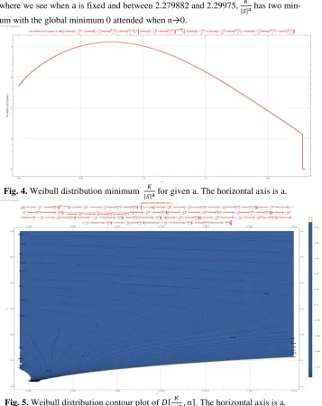
From the minimum plot 𝐾

|𝑆|a in Fig. 4, we see that the asymptotic formula gives

crit-ical value very close to the original shape factors critcrit-ical value 2.279882. By numercrit-ical optimization, we find the minimum of 𝐾

than 0, complying with our guess in section 2.1. This numerical result is supported by the contour plot of the derivative of 𝐾

|𝑆|a with respective to distribution parameter n, Fig.

5, where we see when a is fixed and between 2.279882 and 2.29975, 𝐾

|𝑆|a has two

min-imum with the global minmin-imum 0 attended when n→0.

Fig. 4. Weibull distribution minimum 𝐾

|𝑆|a for given a. The horizontal axis is a.

Fig. 5. Weibull distribution contour plot of 𝐷[ 𝐾

|𝑆|a, 𝑛]. The horizontal axis is a.

When a=2, the minimum of 𝐾

|𝑆|a is 1.9122718704899456695, attended at n=

2.5 Kumaraswamy Distribution Part Two

Boundary β=∞

Return to Kumaraswamy distribution, for a given α, when β→∞, [1] formula (4)-(6) gives the value of the skewness, kurtosis, and the shape factor. We have a similar trick to (12) that:

if log (𝑓(𝑥))𝑥 → log (a), then possibly𝑓(𝑥)~a𝑥1_{. (20)}

Use (20), and confirmed by both 4th _{order and 1}st _{order asymptotic expansion of the}

Gamma function we get the asymptotic order of the boundary shape factor:

limit

𝛼→0 limit𝛽→∞ 𝑆𝐹 ~ 232(1024₇₂₉)𝛼1

3 . (21)

It is a surprise that the shape factor formula (21) for Kumaraswamy distribution and formula (19) for Weibull distribution are the same while their PDF are very different. From equation (13), at the boundary α=0, the shape factor increase from 1 to ∞ when

β turns from 0 to ∞. From equation (21) and [1] equation (4) and (6), at the boundary

β=∞, the shape factor has a minimum value of 1.9122718704899369 𝑤ℎ𝑒𝑛 𝛼 =

0.6411485567602634, increase to ∞ when α turns to 0 or 3.602349425719043. This minimum value for Kumaraswamy distribution is very unusual since it is at the same time the minimum shape factor of the MaxStableDistribution[𝜇,𝜎,𝜉] and the GB2 distribution BetaPrimeDistribution[p,q,α,β] when p=1 ([1] Section 7.1 and Figure 26), three distributions with no relationship apparently.

One experience in this exploration is that when series expansion and heavy substitu-tion are made, the final asymptotic form deducted or guessed need to be validated with the original expression, either by take the symbolic limit of the ratio, or by numerical evaluation of the ratio; different orders of the series expansion arriving at the same form is not enough to guarantee that the form is correct.

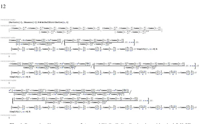
Relationship with Weibull Distribution

Fig. 6. Prove that Kumaraswamy β→∞ and Weibull distribution have identical S K SF.

Since Kumaraswamy distribution can be regarded heuristically as β fold minimum distribution of the power distribution 𝑥𝛼, when β→∞, we guess it should converge in distribution to some extreme value distribution [7][8], and Weibull distribution or the slightly general 𝑀𝑖𝑛𝑆𝑡𝑎𝑏𝑙𝑒𝐷𝑖𝑠𝑡𝑟𝑖𝑏𝑢𝑡𝑖𝑜𝑛 is just that extreme value distribution. Diverse distributions converge to one of the three types of extreme value distribution, so boundary value analysis or asymptotic analysis of the shape factor should arrive at the same or a few typical simple form. We can call distributions with identical SF boundary value formulas asymptotically equivalent distributions, so that asymptotically equivalent distributions will have close or identical parameters when fit a given empir-ical distribution. This is non-trivial when their PDF/CDFs do not have clear relation-ships or similarities.

Minimum Shape Factor Value for Given α or β

Fig. 7. Kumaraswamy distribution minimum shape factor for given β. The horizontal axis is β.

In Fig.7 we see that when β increases from 0 to ∞, the minimum shape factor in-creases from 1 to 1.91227, the minimum value of the shape factor at the boundary β=∞.

Fig. 8. Kumaraswamy distribution minimum shape factor for given α. The horizontal axis is α.

For given shape factor, Fig. 7 and Fig. 8 give the permissible parameters α and β ranges.

2.6 GB2 Distribution

Asymptotic Expression When q→∞

The 𝐺𝐵2([5]), or 𝐵𝑒𝑡𝑎𝑃𝑟𝑖𝑚𝑒𝐷𝑖𝑠𝑡𝑟𝑖𝑏𝑢𝑡𝑖𝑜n[𝑝,𝑞,𝛼,𝛽] shape factor turns to con-stant when q→∞ from Figure 22 and 23 in [1]. From section 2.4 we see that the asymp-totic expression or boundary value of the shape factors can be used as a hint for the original shape factors. So we will utilize asymptotic analysis of the shape factor not for its own sake but as an approximation or initial value to the original shape factor, fol-lowed by numerical correction or validation. Combined with affine transformation in-variance, we can assume q→∞, β=1. From Gamma function 1storder expansion at ∞

we guessed and proved by calculating symbolic limit that:

limit

𝑞→∞ {𝐶𝑀[2], 𝐶𝑀[3], 𝐶𝑀[4]} ≍

{Gamma[𝑞]−2_e−2𝑞_𝑞−1+2𝑞−2_{𝛼, Gamma[𝑞]}−3_e−3𝑞_𝑞−3₂+3𝑞−3_{𝛼, Gamma[𝑞]}−4_e−4𝑞_𝑞−2+4𝑞−_𝛼4_{}. (22)}

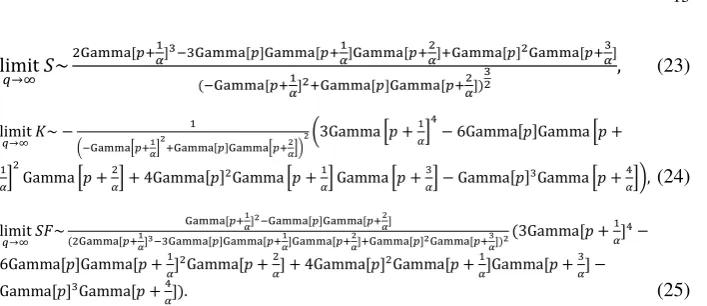
limit_𝑞→∞ 𝑆~2Gamma[𝑝+𝛼1]3−3Gamma[𝑝]Gamma[𝑝+𝛼1]Gamma[𝑝+2𝛼]+Gamma[𝑝]2Gamma[𝑝+3𝛼]

(−Gamma[𝑝+_𝛼1]2_{+Gamma[𝑝]Gamma[𝑝+}2 𝛼])

3

2 , (23)

limit_𝑞→∞ 𝐾~ − 1

(−Gamma[𝑝+1_𝛼]2+Gamma[𝑝]Gamma[𝑝+_𝛼2])2(3Gamma [𝑝 + 1 𝛼]

4

− 6Gamma[𝑝]Gamma [𝑝 +

1 𝛼]

2

Gamma [𝑝 +2_𝛼] + 4Gamma[𝑝]2_{Gamma [𝑝 +}1

𝛼] Gamma [𝑝 + 3

𝛼] − Gamma[𝑝]3Gamma [𝑝 + 4 𝛼]), (24)

limit

𝑞→∞ 𝑆𝐹~

Gamma[𝑝+1_𝛼]2_{−Gamma[𝑝]Gamma[𝑝+}2 𝛼]

(2Gamma[𝑝+1_𝛼]3_{−3Gamma[𝑝]Gamma[𝑝+}1

𝛼]Gamma[𝑝+2𝛼]+Gamma[𝑝]2Gamma[𝑝+𝛼3])2(3Gamma[𝑝 +

1 𝛼]4−

6Gamma[𝑝]Gamma[𝑝 +_𝛼1]2_{Gamma[𝑝 +}2

𝛼] + 4Gamma[𝑝]2Gamma[𝑝 + 1

𝛼]Gamma[𝑝 + 3 𝛼] −

Gamma[𝑝]3_{Gamma[𝑝 +}4

𝛼]). (25)

The simpler formula in the right side of (23)-(25) for S, K, and SF which only in-volve parameters p and α will be our new starting point for studying the minimum and boundary tendencies, and we will call them SB, KB, and SFB, the boundary values of

S, K, and SF for q=∞.

First we have some symbolic limit values for them:

limit

𝑝→0 𝑆𝐹𝐵 =

Gamma[_𝛼2]Gamma[_𝛼4]

Gamma[_𝛼3]2 , (26)

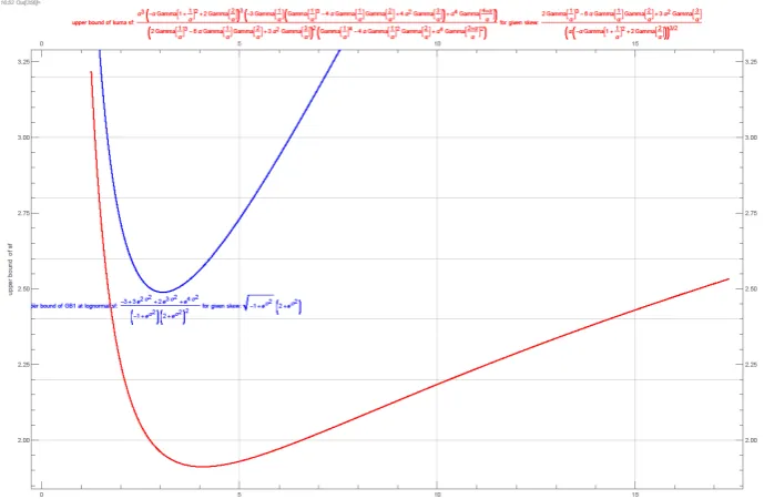
limit_𝛼→∞ 𝑆𝐹𝐵 =PolyGamma[1,𝑝](3PolyGamma[1,𝑝]_{PolyGamma[2,𝑝]}22+PolyGamma[3,𝑝]), (27)

limit_𝑝→∞ 𝑆𝐹𝐵 = ComplexInfinity, limit_𝛼→0 𝑆𝐹𝐵 = ∞. (28)

When p increases from 0 to ∞, equation (27) increases from 2.25 almost linearly to ∞. When α increases from 0 to ∞, equation (26) decreases from ∞ to 1.125. The two directional limits of SFB at the corner of p=0 and α=∞ are different.

Minimum Shape Factor Given p

Now we reduced the parameters numbers to 2, we can similarly use contour plot, partial derivative contour plot, and partial derivative zero points to get minimum shape factor values. For fixed p and α, when q→∞, from the contour plot we see the SF is decreasing, a justification for using q→∞ asymptotic values to calculate the minimum shape factor.

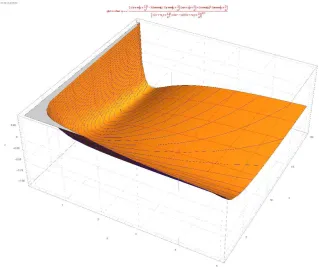
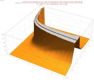
Fig. 10.GB2 shape factor 3D contour plot at q=∞.

Fig. 11. GB2 minimum SF plot for given p, either from asymptotic expression when q→∞ or from empirical formula for numerical optimization results.

The two curves in Fig. 11 have two intersection at p≈0.0016 and p≈0.52, inside the interval [0.0016, 0.52] the empirical curve is slightly lower, and outside of it the asymptotic formula is lower. Checking against the original numerical optimization re-sults shows that when p<1 the asymptotic formula gives better match than the empirical formula, in this case the “human learning” is better than the machine learning from Mathematica 𝐹𝑖𝑛𝑑𝐹𝑜𝑟𝑚𝑢𝑙𝑎.

This minimum shape factor through asymptotic expression converges to 1.125 when p→0, and to 2.4881 when p→∞.

Minimum Shape Factor Given α

Fig. 12. GB2 minimum SF plot for given α, from SFB zero derivative point value or boundary value when p→0.

The composite plot in Fig.12 is checked against the empirical plot Fig. 27 in [1] for

the range of αfrom 0.5 to 1: they matched very well. The tendency of the minimum shape factor given α as shown in Fig. 12 is decreasing from ∞ to 1.125 when α turns

from 0 to ∞.

Fig.11 and Fig.12 can be used to validate the parameter or find the parameters p and

α range when the shape factor is given.

One lesson learned in using series expansion or asymptotic expansion to study the limit of shape factor in the GB2 case is that different order expansions may give differ-ent results. For example, in studying the SFB limit when p→∞, if we use the 0th _order expansion of the Gamma function at ∞, we get limit_𝑝→∞ 𝑆𝐹𝐵~ −₂₅1𝑝𝛼, an absurd negative

number; if we use 1st _{order expansion, and the substitution (𝑝 +}𝑧 𝛼)

−𝑜+𝑛(𝑝+_𝛼𝑧)_→

𝑒𝑛𝑧𝛼𝑝−o+𝑛(𝑝+𝛼𝑧), we get limit

𝑝→∞ 𝑆𝐹𝐵~ − 1

4𝛼𝑝−2, different but still negative. But for the 2 nd_,

3rd_{, 4}th_{, and 5}th _{order expansions, we get the same} limit 𝑝→∞ 𝑆𝐹𝐵~

4

3. We may hurriedly

con-clude that the expansion converged when using above 2nd _{order expansions. Symbolic}

in a summation expression. So it need to be confirmed by other means, such as numer-ical calculation and graphnumer-ical plot. Plot of the 5th _{order expansion SFB crashed}

Mathe-matica kernel, and numerical calculation caused overflow. It is found that MatheMathe-matica cannot calculate Gamma[10.^14] in arbitrary-precision arithmetic due to a restriction of maximum numbers allowed in this format. That may be why its plots have many void portions. So verification by alternative software is desired: there is a package MPMATH in SYMPY that can be tested in IPython, which can calculate gamma(10**14) or even gamma(10**100). For α=1, p increasing, MPMATH calcu-lated SFB is also increasing and follows some pattern until p=10**21, after that the calculated SFB fluctuates between positive and negative numbers; for p=10**55, 10**100000, 10**1000000, it gives 0: results hard to reconcile.

When plot the zero value contour in the parameter space of p and α of the partial derivatives of SFB with respective to α and p, we see that the former is higher than the latter, Fig.13.

Fig. 13. D[SFB,α] and D[SFB,p] 0 contour plot.

Characteristic Number

From equation (22) take more symbolic limit we get:

limit_𝑞→∞ 𝐶𝑀[2]~𝑞−𝛼2−Gamma[𝑝+ 1 𝛼]

2

+Gamma[𝑝]Gamma[𝑝+_𝛼2]

Gamma[𝑝]2 , (29)

limit_𝑞→∞ 𝐶𝑀[3]~𝑞−3_𝛼2Gamma[𝑝+𝛼1] 3

−3Gamma[𝑝]Gamma[𝑝+1_𝛼]Gamma[𝑝+2_𝛼]+Gamma[𝑝]2_Gamma[𝑝+3 𝛼]

Gamma[𝑝]3 , (30)

limit_𝑞→∞ 𝐶𝑀[4]~_Gamma[𝑝]𝑞−4𝛼 4(−3Gamma [𝑝 +

1 𝛼]

4

+ 6Gamma[𝑝]Gamma [𝑝 +

1 𝛼]

2

Gamma [𝑝 +_𝛼2] − 4Gamma[𝑝]2_{Gamma [𝑝 +}1

𝛼] Gamma [𝑝 + 3 𝛼] +

Gamma[𝑝]3_{Gamma[𝑝 +}4

𝛼]). (31)

From equation (29)-(31) and similarly by working with limit of each individual fac-tors for a production expression we get:

limit

𝑝→0 limit 𝑞→∞ 𝐾

𝑆a~Gamma[𝑝]1− a

2Gamma[2

𝛼]

−2+3a_2Gamma[3

𝛼]−aGamma [ 4

𝛼], (32)

limit

𝛼→0 limit 𝑞→∞ 𝐾 𝑆a~2

3a𝑝−a−1

2 3a(12−𝑝)𝜋a−24 (24+3a

33a ) 1

𝛼𝛼(a−2)(2𝑝−1)4 Gamma[𝑝]1−a2. (33)

From equation (32) we know the characteristic number of GB2 distribution is still 2: whose min 𝐾

𝑆a→ 0 when a>2, q→∞, and p→0.

Equation (33) says that at the boundary of α=0 and q=∞, an identical to the omni-present Weibull distribution critical value a=2.279348388468605 exit: above it,

limit

𝛼→0 limit 𝑞→∞ 𝐾

𝑆a~0, but below it, limit_𝛼→0 limit _{𝑞→∞ 𝑆}𝐾a~∞. So the α=0 and the p=0 boundaries

have different directional critical values with the p=0 boundary one smaller and gives the global characteristic number 2 for GB2.

3

Conclusion and Discussions

The conditional minimum of the shape factor for given parameter value or given ex-pression value such as the skewness is useful, but its plot can usually only be obtained through numerical method (as in [1][2]). The simplification of the shape factor through asymptotic approximation can provide a deterministic way of solving the conditional minimum problem. The numerical and analytical method are thus checking and vali-dating each other. In the process of those boundary or limit and minimum analysis, some characteristics of the shape factor (the characteristic number), as well as mysteri-ous relationships of distributions, such as those between Kumaraswamy and Weibull distributions, and between GB2 and Weibull distributions,

𝐵𝑒𝑡𝑎𝑃𝑟𝑖𝑚𝑒𝐷𝑖𝑠𝑡𝑟𝑖𝑏𝑢𝑡𝑖𝑜[1, ∞, 𝛼, 1] ≈ 𝑊𝑒𝑖𝑏𝑢𝑙𝑙𝐷𝑖𝑠𝑡𝑟𝑖𝑏𝑢𝑡𝑖𝑜𝑛[𝛼, 1] ≈

GB1 distribution, similar to GB2 distribution, has simpler form of moment than cen-tral moment; those kind of shape factor by moment, such as 𝑀[2]∗𝑀[4]_𝑀[3]2 , is easier to work at, and arrive at identical boundary or asymptotic limit formulas as we get of GB2 or Kumaraswamy distribution. The asymptotic limit seems even out the differences be-tween moment and central moment in this case.

So whenever asymptotic limit can be calculated and has simpler form, it will be an invaluable tool for studying the original shape factor. This substitute method is also applicable when the limit of distribution PDF/CDF is hard to get, we can work on the SF limit instead; or when some but not all of S, K, and SF have infinite limit, we can change/modify to study the one with finite limit which can reveal additional

infor-mation of the distribution (“structure inside the singularity”).

Heuristically or by analogy we can think S as a first order derivative, K as a shifted first order derivative, and SF as a second order derivative, describing the convexity or curvature of the distribution PDF, so in some cases SF should have simpler form than S or K, a reason for using it as the alternative.

The method in Fig.2 can be used to study GB2 minimum shape factor with given product of 𝑝𝛼, and we guess the peak in [1] Fig. 27 is the impact of the zero value contour curve of the skewness. Some deduction of the asymptotic value of the shape factor of GH is in [2], but the detailed study for all these will be in a subsequent paper.

Conflict of Interest

The author declare no conflict of interest.

References

1. Wang FX (2018) What determine EP curve shape? doi:10.13140/RG.2.2.30056.11523 2. Wang FX (2019) What determines EP curve shape? In: Dr. Bruno Carpentieri (ed) Applied

Mathematics. https://cdn.intechopen.com/pdfs/64962.pdf

3. Hardy GH, Wright EM (1979) An Introduction to the Theory of Numbers, 5th ed. Oxford, England: Clarendon Press

4. Marichev O, Trott M (2013) The Ultimate Univariate Probability Distribution Explorer. http://blog.wolfram.com/2013/02/01/the-ultimate-univariate-probability-distribution-ex-plorer/. Accessed 6 June 2018

5. McDonald JB, Sorensen J, Turley PA (2011) Skewness and kurtosis properties of income distribution models. LIS Working Paper Series, No. 569. Review of Income and Wealth. doi:10.1111/j.1475-4991.2011.00478.x. https://pdfs.seman-ticscholar.org/eabd/0599193022dfc65ca00f28c8a071e43edc32.pdf

6. McDonald JB (1984) Some Generalized Functions for the Size Distribution of Income. Econometrica 52(3):647-663

7. Embrechts P, Kluppelberg C, Mikosch T (1997) Modelling Extremal Events for Insurance and Finance. Springer. doi:10.1007/978-3-642-33483-2