Munich Personal RePEc Archive
A unit root test based on smooth
transitions and nonlinear adjustment
Hepsag, Aycan
Istanbul University
5 October 2017
1
A unit root test based on smooth transitions and nonlinear
adjustment
Aycan Hepsag*
Abstract
In this paper, we develop a new unit root testing procedure which considers jointly for
structural breaks and nonlinear adjustment. The structural breaks are modelled by means of a
logistic smooth transition function and nonlinear adjustment is modelled by means of an
ESTAR model. The empirical size of test is quite close to the nominal one and in terms of
power; the new unit root test is generally superior to the alternative test. The new unit root test
presents good size properties and does not lead to over-rejections of the null hypothesis of the
unit root.
Keywords: Smooth transitions, nonlinearity, unit root, ESTAR
JEL Classification: C12, C22
* Istanbul University, Faculty of Economics, Department of Econometrics, Tel.: +90 212 440 01 60, Beyazıt,
2
1. Introduction
In the last forty years, the time series analysis of models with unit roots has increasingly
become one of the major topics for the investigators and practitioners to understand the
response of economic systems to shocks. The first tests for unit root were proposed by Fuller
(1976) and Dickey and Fuller (1979). However, it is well known that the presence of
structural breaks and nonlinearities in time series might affect the power of the traditional unit
root tests. Accordingly, the Dickey-Fuller test fails to reject the null hypothesis of unit root
and these types of tests would be powerless to separate the behaviour of a unit process from
the behaviour of a stationary process with structural breaks.
Perron (1989) proposed a unit root test which takes into account structural breaks
exogenously in the deterministic components and displayed that the traditional unit roots tests
detect incorrectly that the series have a unit root when in fact they are stationary with
structural breaks. Apart from Perron (1989), many authors have developed unit root tests in
order to take into account structural breaks (Zivot and Andrews (1992); Lumsdaine and Papell
(1997); Lee and Strazicich (2003). The main feature of these unit root tests is that the
deterministic structural changes are assumed to occur instantaneously, only in certain points
of time.
Nonetheless, individual agents can react simultaneously to a given economic stimulus; while
some may be able to react instantaneously and so will adjust with different time lags. Thus,
when considering aggregate behaviour, the time path of structural changes in economic series
is likely to be better captured by a model whose deterministic component permits gradual
rather than instantaneous adjustment between different values (Leybourne, Newbold and
3 consider smooth rather than a sudden change. The main idea behind of these tests is that
nonlinearities can be present in time series as an asymmetric speed of mean reversion and
autoregressive parameter varies depending upon the values of a variable. This nonlinear
behaviour implies that there is a central regime where the series behave as a unit root whereas
for values outside the central regime, the variable tends to revert to the equilibrium (Cuestas
and Ordóñez, 2014).
The nonlinear dynamics for unit root testing procedures and the joint analysis of nonlinearity
and nonstationarity have been popularised since about the last twenty years. Kapetanios, Shin
and Snell (2003) proposed a unit root test within an exponential smooth transition
autoregressive (ESTAR) model. Apart from Kapetanios, Shin and Snell (2003), Sollis (2009),
Kruse (2011) present invaluable contributions to the testing of unit roots considering
nonlinearity. Although these studies consider asymmetric speed of mean reversion, they do
not take into account nonlinearities in the deterministic components.
On the other hand, Christopoulos and León-Ledesma (2010) developed tests for unit roots that
account jointly for structural breaks and nonlinear adjustment. The prominent contribution of
unit root test of Christopoulos and León-Ledesma (2010) is that this test takes into account
asymmetric speed of mean reversion, as well as structural changes in the intercept,
approximated by means of a Fourier function. Cuestas and Ordóñez (2014) also proposed a
unit root test which extends the unit root test of Leybourne, Newbold and Vougas (1998) and
takes into account both sources of nonlinearities, i.e. in the deterministic components,
approximated by a logistic smooth transition function not only in the intercept, but also in the
4 In this paper, we develop a new unit root testing procedure which considers jointly for
structural breaks and nonlinear adjustment. In our proposed test, structural breaks are
modelled by means of a logistic smooth transition function that allows in the intercept, in the
intercept under a fixed slope and in the intercept and slope terms. Nonlinear adjustment is
modelled by means of an ESTAR model as suggested by Kruse (2011).
The rest of the paper is organized as follows: Section 2 describes the proposed test statistics
and provides asymptotic critical values. Section 3 presents the results of power and size of our
proposed test via Monte Carlo simulation experiments. The last section concludes the paper.
2. The Unit Root Test
In this section, we propose a unit root test which accounts jointly for structural breaks and
nonlinear adjustment. The test, which is considered as an alternative to Leybourne et. al.
(1998) and Kruse (2011), attempts to model the structural change as a smooth transition
between different regimes over time and also model the nonlinearities by means of ESTAR
model suggested by Kruse (2011).
In order to develop the new unit root testing strategy, we consider the following three logistic
smooth transition models by following Leybourne, Newbold and Vougas (1998):
Model A: yt
1 2St
, vt (1)Model B: yt
1 1t
2St
, vt (2)5 where vt is error term which is normally distributed with zero mean and unit variance and
,t
S is the logistic smooth transition function, based on a sample of size T.
1, 1 exp
t
S tT
0 (4)The parameter determines the timing of the transition midpoint and the speed of transition
is determined by the parameter
. If we assume vt is a zero-mean I
0 process, then inmodel A yt is stationary around a mean which changes from the initial value
1 to the finalvalue
1 2. Model B is similar to Model A, with the intercept changing from
1 to
1 2, but it allows for a fixed slope term. Finally, in Model C, in addition to the change in
intercept from
1 to
1 2, the slope also changes contemporaneously, and with the samespeed of transition
1 to
1 2.In this paper, we also follow a similar way to the approach of Cuestas and Ordóñez (2014)
who propose to apply the unit root test of Kapetanios, Shin and Snell (2003) to the residuals
of Equation (3) which considers the smooth breaks in the intercept and slope.
The null of unit root hypothesis may be stated as follows:
0: t t, t t 1 t
H y
(5)where
t is assumed to be an I
0 process with zero mean. In our proposed unit root test, the6 least squares (NLS) algorithm for estimating model A, B and C, and then we compute the
NLS residuals.
Model A: vˆt yt ˆ1 ˆ2St
ˆ,ˆ (6)Model B: vˆt yt ˆ1 ˆ1tˆ2St
ˆ,ˆ (7)Model C: vˆt yt ˆ1 ˆ1tˆ2St
ˆ,ˆ ˆ2tSt
ˆ,ˆ (8)In the second step, we apply the unit root test of Kruse (2011) to the residuals obtained in the
first step. We allow for a nonzero location parameter c by following Kruse (2011) in the
ESTAR model which is modified to our strategy as the following form:
2
1 1
ˆt ˆt 1 exp ˆt t
v v v c
(9)
where ˆvt is the estimated NLS residuals in the first step. Kruse (2011) proposes a first order
Taylor approximation for equation (9) and obtains the auxiliary regression shown at equation
(10).
3 2
1 1 2 1 1
ˆt ˆt ˆt p i ˆt i t
i
v
v
v
v
(10)
In the auxiliary regression (10), the null hypothesis could be constituted H0:
1 20against H1:
10,
2 0. It can be remarked that one parameter is one-sided and the otherone is two-sided under the alternative hypothesis so a standard Wald type would be
7 Abadir and Distaso (2007), the one-sided parameter is orthogonalized with respect to the
two-sided one. The test statistics of our new procedure are computed as a modified Wald type test
which builds upon the one-sided parameter and the transformed two-sided parameter:
2
2 2
21 21 1
22 2 1 1
11 11 11
ˆ
ˆ ˆ ˆ ˆ ˆ
ˆ ˆ ˆ 1 0 ˆ
SNL SNL SNL
(11)
which are the new statistics for a unit root hypothesis against nonlinear and stationary with
one smooth break.
ˆ22,
ˆ11 and
ˆ21 are the elements of Variance-Covariance matrix. Wedenote the value of test statistics as
SNL if Model A is used to construct the vˆt, SNL ifModel B is used and
SNL if Model C is used.As mentioned by Leybourne, Newbold and Vougas (1998), we assume the residuals vt are
zero-mean I
0 processes, and then yt are also stationary processes in models A, B and C.Therefore, the asymptotic distributions of
SNL, SNL and
SNL statistics have the sameproperties with the
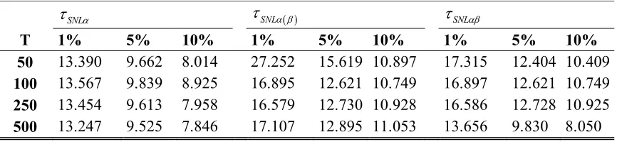
statistic of Kruse (2011). (For proofs, see Appendix of Kruse (2011)).Thus, the critical values of
SNL, SNL and
SNL test statistics have been obtained viastochastic simulations at 1%, 5% and 10% significance levels based on 50,000 replications for
50,100, 250, 500
8
Table 1: Critical Values
SNL
SNL
SNLT 1% 5% 10% 1% 5% 10% 1% 5% 10%
50 13.390 9.662 8.014 27.252 15.619 10.897 17.315 12.404 10.409
100 13.567 9.839 8.925 16.895 12.621 10.749 16.897 12.621 10.749
250 13.454 9.613 7.958 16.579 12.730 10.928 16.586 12.728 10.925
500 13.247 9.525 7.846 17.107 12.895 11.053 13.656 9.830 8.050
3. Monte Carlo Study
This section involves the Monte Carlo investigation of the size properties and power
performance of our new unit root test and also the power comparison of the new test with
Kruse (2011) test.
First, we study the empirical size of test for different sample sizes i.e. T 50,100 with a
nominal size of 0.05. We generate the DGP as follows.
1 0
, , 0 ~ 0,1
t t t t t t
y
NIID (12)The results of empirical size of test, based on 5000 replications, are presented in Table 2. In
general, we could conclude that the empirical size of test is quite close to the nominal one,
5%. A significant size distortion is only determined for T 50 for SNL test. Nonetheless,
the size distortion disappears for T 100.
Table 2: Size Properties of Test
T
SNL SNL
SNL50 0.059 0.017 0.046
[image:9.612.93.521.622.672.2]9 Next, we investigate the power of
SNL, SNL ,
SNL tests based on the following models,respectively:
10
1 1 exp t t y v t T
(13)
10
1 10
1 exp
t t
y t v
t T
(14)
10
10
1 10
1 exp 1 exp
t t t
y t v
t T t T
(15)
2
1 1 exp 1
t t t t
v v v c
(16)
with 1.0, 0.5 and 1.5. The location parameter c is allowed by drawing from a
uniform distribution with lower and upper bound of 5 10
and 5 10 , respectively.
Analogously, the parameter is allowed by drawing from a uniform distribution with lower
and upper bound of
0.001,0.01 with slow transition between regimes
l and
0.01,0.1
with fast transition between regimes
h , respectively. The nominal size of the tests aredetermined at 0.05, the number of replications is 5000 and the sample size is considered for
50,100
T . The results of power experiments and power comparison with Kruse (2011) test
10
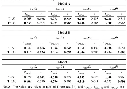
Table 3: Power Experiments and Comparison
Model A
5,
c
l c5,
h c10,
l c10,
hSNL
SNL
SNL
SNL T=50 0.068 0.168 0.795 0.835 0.260 0.138 0.938 0.815
T=100 0.333 0.304 0.964 0.986 0.448 0.265 1.000 0.983
Model B
5,
c
l c5,
h c10,
l c10,
h
SNL
SNL SNL SNL
T=50 0.042 0.166 0.396 0.642 0.050 0.138 0.998 0.854
T=100 0.116 0.134 0.514 0.692 0.846 0.286 0.704 1.000
Model C
5,
c
l c5,
h c10,
l c10,
hSNL
SNL
SNL
SNL T=50 0.077 0.141 0.338 0.227 0.209 0.026 1.000 0.760
T=100 0.404 0.170 0.796 0.507 0.319 0.043 0.773 0.998
Notes: The values are rejection rates of Kruse test
and
SNL, SNL and
SNL testsand bold values display the cases where each test performs better. In power experiments we consider
dt1 statistic for model A and 1t
d t
statistics for models B and C.
The results of the power experiments and comparison show that the new unit root test is
generally superior to the Kruse test. Only in some cases where the unit root test is applied for
Model B, the Kruse test performs better than SNL test.
4. Conclusions
In this paper, we develop a new unit root testing procedure which considers jointly for
structural breaks and nonlinear adjustment. The empirical size of test is quite close to the
nominal one and in terms of power; the new unit root test is generally superior to the Kruse
test. The new unit root test presents good size properties and does not lead to over-rejections
11
References
Abadir K. M., and W. Distaso. 2007. Testing joint hypotheses when one of the alternatives is
one-sided. Journal of Econometrics 140: 695–718.
Christopoulos, D., and M. A. León-Ledesma. 2010. Smooth breaks and non-linear mean
reversion: post-Bretton-Woods real exchange rates. Journal of International Money and
Finance 29: 1076–1093.
Cuestas, J. C., and J. Ordóñez. 2014. Smooth transitions, asymmetric adjustment and unit
roots. Applied Economics Letters 21: 969–972.
Dickey, D. A. And W. A. Fuller. 1979. Distribution of the estimators for autoregressive time
Series with a unit root. Journal of the American Statistical Association 84: 427–431.
Fuller, W. A. 1976. Introduction of statistical time series. Wiley, New York.
Kapetanios, G., Y. Shin, and A. Snell. 2003. Testing for a unit root in the nonlinear STAR
framework. Journal of Econometrics 112: 359–379.
Kruse, R. 2011. A new unit root test against ESTAR based on a class of modified
statistics. Statistical Papers 52: 71–85.
Lee, J., and M. C. Strazicich. 2003. Minimum Lagrange multiplier unit root test with two
12 Leybourne, S., P. Newbold, and D. Vougas. 1998. Unit roots and smooth transitions. Journal
of Time Series Analysis 19: 83–97.
Lumsdaine, R.L., Papell, D.H. 1997. Multiple trend breaks and the unit-root hypothesis.
Review of Economics and Statistics. 79, 212–218.
Sollis, R. 2009. A simple unit root test against asymmetric STAR nonlinearity with an
application to real exchange rates in Nordic countries. Economic Modelling 26: 118–125.
Perron, P. 1989. The great crash, the oil price shock and the unit root hypothesis.
Econometrica 57: 1361–1401.
Zivot, E., and D. W. K. Andrews. 1992. Further evidence on the Great Crash, the oil-price
shock, and the unit-root hypothesis. Journal of Business and Economic Statistics 10: 251–