Learning Latent Trees with Stochastic Perturbations and Differentiable Dynamic Programming

5508

Learning Latent Trees with Stochastic Perturbations

and Differentiable Dynamic Programming

Caio Corro Ivan Titov

ILCC, School of Informatics, University of Edinburgh ILLC, University of Amsterdam

[email protected] [email protected]

Abstract

We treat projective dependency trees as latent variables in our probabilistic model and induce them in such a way as to be beneficial for a downstream task, without relying on any direct tree supervision. Our approach relies on Gum-bel perturbations and differentiable dynamic programming. Unlike previous approaches to latent tree learning, we stochastically sample global structures and our parser is fully differ-entiable. We illustrate its effectiveness on sen-timent analysis and natural language inference tasks. We also study its properties on a syn-thetic structure induction task. Ablation stud-ies emphasize the importance of both stochas-ticity and constraining latent structures to be projective trees.

1 Introduction

Discrete structures are ubiquitous in the study of natural languages, for example in morphology, syntax and discourse analysis. In natural language processing, they are often used to inject linguistic prior knowledge into statistical models. For exam-ples, syntactic structures have been shown benefi-cial in question answering (Cui et al.,2005), senti-ment analysis (Socher et al.,2013), machine trans-lation (Bastings et al.,2017) and relation extrac-tion (Liu et al., 2015), among others. However, linguistic tools producing these structured repre-sentations (e.g., syntactic parsers) are not avail-able for many languages and not robust when ap-plied outside of the domain they were trained on (Petrov et al., 2010; Foster et al., 2011). More-over, linguistic structures do not always seem suitable in downstream applications, with sim-pler alternatives sometimes yielding better perfor-mance (Wang et al.,2018).

Indeed, a parallel line of work focused on induc-ing task-specific structured representations of lan-guage (Naradowsky et al.,2012;Yogatama et al.,

2017;Kim et al.,2017;Liu and Lapata,2018; Nic-ulae et al., 2018). In these approaches, no syn-tactic or semantic annotation is needed for train-ing: representation is induced from scratch in an end-to-end fashion, in such a way as to benefit a given downstream task. In other words, these ap-proaches provide an inductive bias specifying that (hierarchical) structures are appropriate for repre-senting a natural language, but do not make any further assumptions regarding what the structures represent. Structures induced in this way, though useful for the task, tend not to resemble any ac-cepted syntactic or semantic formalisms (Williams et al.,2018a). Our approach falls under this cate-gory.

In our method, projective dependency trees (see Figure3 for examples) are treated as latent vari-ables within a probabilistic model. We rely on differentiable dynamic programming (Mensch and Blondel,2018) which allows for efficient sampling of dependency trees (Corro and Titov,2019). Intu-itively, sampling a tree involves stochastically per-turbing dependency weights and then running a re-laxed form of the Eisner dynamic programming al-gortihm (Eisner,1996). A sampled tree (or its con-tinuous relaxation) can then be straightforwardly integrated in a neural sentence encoder for a target task using graph convolutional networks (GCNs,

Kipf and Welling, 2017). The entire model, in-cluding the parser and GCN parameters, are es-timated jointly while minimizing the loss for the target task.

reinforce-ment learning (Yogatama et al.,2017;Nangia and Bowman, 2018; Williams et al., 2018a) or does not treat the latent structure as a random vari-able (Peng et al., 2018). Niculae et al. (2018) marginalizes over latent structures, however, this necessitates strong sparsity assumptions on the posterior distributions which may inject undesir-able biases in the model. Overall, differential dy-namic programming has not been actively studied in the task-specific tree induction context. Most previous work also focused on constituent trees rather than dependency ones.

We study properties of our approach on a syn-thetic structure induction task and experiment on sentiment classification (Socher et al., 2013) and natural language inference (Bowman et al.,2015). Our experiments confirm that the structural bias encoded in our approach is beneficial. For ex-ample, our approach achieves a 4.9% improve-ment on multi-genre natural language inference (MultiNLI) over a structure-agnostic baseline. We show that stochastisticity and higher-order statis-tics given by the global inference are both impor-tant. In ablation experiments, we also observe that forcing the structures to be projective dependency trees rather than permitting any general graphs yields substantial improvements without sacrific-ing execution time. This confirms that our induc-tive bias is useful, at least in the context of the considered downstream applications.1 Our main contributions can be summarized as follows:

1. we show that a latent tree model can be esti-mated by drawing global approximate sam-ples via Gumbel perturbation and differen-tiable dynamic programming;

2. we demonstrate that constraining the struc-tures to be projective dependency trees is beneficial;

3. we show the effectiveness of our approach on two standard tasks used in latent structure modelling and on a synthetic dataset.

2 Background

In this section, we describe the dependency pars-ing problem and GCNs which we use to incorpo-rate latent structures into models for downstream tasks.

1_{The Dynet code for differentiable dynamic programming}

is available at https://github.com/FilippoC/ diffdp.

2.1 Dependency Parsing

Dependency trees represent bi-lexical relations be-tween words. They are commonly represented as directed graphs with vertices and arcs correspond-ing to words and relations, respectively.

Letx = x0. . . xn be an input sentence withn words where x0 is a special root token. We de-scribe a dependency tree of x with its adjacency matrixT ∈ {0,1}n×n _whereT

h,m = 1iff there is a relation from head wordxh to modifier word xm. We writeT(x)to denote the set of trees com-patible with sentencex.

We focus on projective dependency trees. A dependency tree T is projective iff for every arc

Th,m = 1, there is a path with arcs inT fromxhto each wordxisuch thath < i < morm < i < h. Intuitively, a tree is projective as long as it can be drawn above the words in such way that arcs do not cross each other (see Figure 3). Similarly to phrase-structure trees, projective dependency trees implicitly encode hierarchical decomposition of a sentence into spans (‘phrases’). Forcing trees to be projective may be desirable as even flat span struc-tures can be beneficial in applications (e.g., encod-ing multi-word expressions). Note that actual syn-tactic trees are also, to a large degree, projective, especially for such morphologically impoverished languages as English. Moreover, restricting the space of the latent structures is important to ease their estimation. For all these reasons, in this work we focus on projective dependency trees.

In practice, a dependency parser is given a sen-tencexand predicts a dependency treeT _{∈ T}(x) for this input. To this end, the first step is to com-pute a matrix W ∈ Rn×n that scores each

de-pendency. In this paper, we rely on a deep dotted attention network. Let e0. . .en be embeddings associated with each word of the sentence.2 We followParikh et al.(2016) and compute the score for each head-modifier pair(xh, xm)as follows:

Wh,m= MLPhead(eh)>MLPmod(em)+bh-m, (1)

whereMLPhead_andMLPmod _{are multilayer} per-ceptrons, and bh-m is a distance-dependent bias, letting the model encode preference for long or short-distance dependencies. The conditional probability of a treepθ(T|x) is defined by a

log-2_{The embeddings can be context-sensitive, e.g., an RNN}

linear model:

pθ(T|x) =

exp(P

h,mWh,mTh,m)

P

T0_∈T(x)exp( P

h,mWh,mT_h,m0 ) .

When tree annotation is provided in dataD,

net-works parametersθare learned by maximizing the log-likelihood of annotated trees (Lafferty et al.,

2001).

The highest scoring dependency tree can be duced by solving the following mathematical pro-gram:

T = arg max T∈T(x)

X

h,m

Wh,mTh,m. (2)

If T(x) is restricted to be the set of projective dependency trees, this can be done efficiently in

O(n3_{)using the dynamic programming algorithm} ofEisner(1996).

2.2 Graph Convolutional Networks

Graph Convolutional Networks (GCNs, Kipf and Welling, 2017; Marcheggiani and Titov, 2017) compute context-sensitive embeddings with re-spect to a graph structure. GCNs are composed of several layers where each layer updates vertices representations based on the current representa-tions of their neighbors. In this work, we fed the GCN with word embeddings and a tree sampleT. For each word xi, a GCN layer produces a new representation relying both on word embedding of

xi and on embeddings of its heads and modifiers inT. Multiple GCN layers can be stacked on top of each other. Therefore, a vertex representation in a GCN withklayers is influenced by all vertices at a maximum distance ofkin the graph. Our GCN is sensitive to arc direction.

More formally, letE0 =e0 · · · en, where is the column-wise concatenation operator, be the input matrix with each column corresponding to a word in the sentence. At each GCN layert, we compute:

Et+1 =σf(Et) +g(Et)T +h(Et)T>

,

where σ is an activation function, e.g. ReLU. Functions f(), g() and h() are distinct multi-layer perceptrons encoding different types of rela-tionships: self-connection, head and modifier, re-spectively (hyperparameters are provided in Ap-pendix A). Note that each GCN layer is easily parallelizable on GPU both over vertices and over batches, either with latent or predefined structures.

(a)

x T y

(b)

x T T _x0

0 y

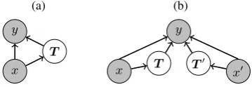
Figure 1: The two directed graphical models used in this work. Shaded and unshaded nodes represent ob-servable and unobob-servable variables, respectively. (a) In the sentence classification task, the outputy is con-ditioned on the input and the latent tree.(b)In the nat-ural language inference task, the output is conditioned on two sentences and their respective latent trees.

3 Structured Latent Variable Models

In the previous section, we explained how a de-pendency tree is produced for a given sentence and how we extract features from this tree with a GCN. In our model, we assume that we do not have access to gold-standard trees and that we want to induce the best structure for the down-stream task. To this end, we introduce a prob-ability model where the dependency structure is a latent variable (Section 3.1). The distribution over dependency trees must be inferred from the data (Section 3.2). This requires marginalization over dependency trees during training, which is in-tractable due to the large search space.3 Instead, we rely on Monte-Carlo (MC) estimation.

3.1 Graphical Model

Letxbe the input sentence, y be the output (e.g. sentiment labelling) andT(x)be the set of latent structures compatible with inputx. We construct a directed graphical model wherexandyare ob-servable variables, i.e. their values are known dur-ing traindur-ing. However, we assume that the proba-bility of the outputyis conditioned on a latent tree T _{∈ T}(x), a variable that is not observed during training: it must be inferred from the data. For-mally, the model is defined as follows:

pθ(y|x) =Epθ(T|x)[p(y|x,T)] (3)

= X

T∈T(x)

pθ(T|x)×pθ(y|x,T),

whereθ denotes all the parameters of the model. An illustration of the network is given in Fig-ure1a.

3_{This marginalization is a sum of the network outputs over}

3.2 Parameter Estimation

Our probability distributions are parameterized by neural networks. Their parameters θare learned via gradient-based optimization to maximize the log-likelihood of (observed) training data. Unfor-tunately, estimating the log-likelihood of observa-tion requires computing the expectaobserva-tion in Equa-tion3, which involves an intractable sum over all valid dependency trees. Therefore, we propose to optimize a lower bound on the log-likelihood, de-rived by application of Jensen’s inequality which can be efficiently estimated with the Monte-Carlo (MC) method:

logpθ(yi|xi) = logET∼pθ(T|xi)[pθ(y

i_{|T, x}i_)]

≥ET∼pθ(T|xi)[logpθ(y

i

|T, xi)]. (4)

However, MC estimation introduces a non-differentiable sampling function T _∼ pθ(T|xi) in the gradient path. Score function estimators have been introduced to bypass this issue but suf-fer from high variance (Williams,1987;Fu,2006;

Schulman et al., 2015). Instead, we propose to reparametrize the sampling process (Kingma and Welling,2014), making it independent of the learned parameterθ : in such case, the sampling function is outside of the gradient path. To this end, we rely on the Perturb-and-MAP framework (Papandreou and Yuille, 2011). Specifically, we perturb the potentials (arc weights) with samples from the Gumbel distribution and compute the most probable structure with the perturbed poten-tials:

Gh,m∼ G(0,1), (5)

f

W =W +G, (6)

T = arg max T∈T(x)

X

h,m

Th,mWf_h,m. (7)

Each element of the matrix G _∈ Rn×n contains

random samples from the Gumbel distribution4 which is independent from the network parameters

θ, hence there is no need to backpropagate through this path in the computation graph. Note that, unlike the Gumbel-Max trick (Maddison et al.,

2014), sampling with Perturb-and-MAP is approx-imate, as the noise is factorizable: we add noise to individual arc weights rather than to scores of entire trees (which would not be tractable). This

4_{That is Gh,m = −log(−log(Uh,m))whereUh,mis}

sampled from the uniform distribution on the interval(0,1).

Algorithm 1This function computes the chart val-ues for items of the form [i, j,→,⊥] by search-ing the set of antecedents that maximizes its score. Because these items assume a dependency fromxi toxj, we addWi,hto the score.

1: functionBUILD-URIGHT(i, j,Wf)

2: s_←null-initialized vec. of sizej₋i

3: fori≤k < jdo

4: si−k←[i, k,→,>] + [k+ 1, j,←,>]

5: b_←ONE-HOT-ARGMAX(s)

6: BACKPTR[i, j,→,⊥]←b

7: WEIGHT[i, j,→,⊥]←b>s+Wj,i

Algorithm 2 If item [i, j,_→,_⊥] has contributed the optimal objective, this function setsTi,j to1. Then, it propagates the contribution information to its antecedents.

1: functionBACKTRACK-URIGHT(i, j,T) 2: Ti,j ←CONTRIB[i, j,→,⊥]

3: b_← BACKPTR[i, j,→,⊥] 4: fori≤k < jdo

5: CONTRIB[i, k,→,>]←+ bi−kTi,j

6: CONTRIB[k+ 1, j,←,>]←+ bi−kTi,j

is the first source of bias in our gradient estima-tor. The maximization in Equation7can be com-puted using the algorithm of Eisner (1996). We stress that the marginalization in Equation 3 and MC estimated sum over trees capture high-order statistics, which is fundamentally different from computing edge marginals, i.e. structured atten-tion (Kim et al., 2017). Unfortunately, the esti-mated gradient of the reparameterized distribution over parse trees is ill-defined (either undefined or null). We tackle this issue in the following section.

4 Differentiable Dynamic Programming

Neural networks parameters are learned using (variants of) the stochastic gradient descent algo-rithm. The gradient is computed using the back-propagation algorithm that rely on partial deriva-tive of each atomic operation in the network.5 The perturb-and-MAP sampling process relies on the dependency parser (Equation 7) which contains ill-defined derivatives. This is due to the usage of constrained arg max operations (Gould et al.,

5_{There are some exception where a sub-derivative is}

2016;Mensch and Blondel,2018) in the algorithm ofEisner(1996). LetLbe the training loss, back-propagation is problematic because of the follow-ing operation:

∂L

∂Wf

= ∂L

∂T

∂T

∂Wf

where ∂T ∂Wf

is the partial derivative with respect to the dependency parser (Equation7) which is null almost everywhere, i.e. there is no descent direc-tion informadirec-tion. We follow previous work and use a differentiable dynamic programming surro-gate (Mensch and Blondel,2018;Corro and Titov,

2019). The use of the surrogate is the second source of bias in our gradient estimation.

4.1 Parsing with Dynamic Programming

The projective dependency parser ofEisner(1996) is a dynamic program that recursively builds a chart of items representing larger and larger spans of the input sentence. Items are of the form [i, j, d, c]where: 0 ≤ i ≤ j ≤ nare the bound-aries of the span; d _{∈ {→},_←} is the direction of the span, i.e. a right span → (resp. left span ←) means that all the words in the span are de-scendants ofxi(resp. xj) in the dependency tree; c _{∈ {>},_⊥}indicates if the span is complete (>) or incomplete (⊥) in its direction. In a complete right span, xj cannot have any modifiers on its right side. In a complete left span,xicannot have any modifier on its left side. A set of deduction rules defines how the items can be deduced from their antecedents.

The algorithm consists of two steps. In the first step, items are deduced in a bottom-up fashion and the following information is stored in the chart: the maximum weight that can be obtained by each item and backpointers to the antecedents that lead to this maximum weight (Algorithm1). In the sec-ond step, the backpointers are used to retrieve the items corresponding to the maximum score and values inT are set accordingly (Algorithm2).6

4.2 Continuous Relaxation

Theone-hot-argmaxoperation on line5in Algo-rithm1can be written as follows:

arg max b≥0

X

k

bksk s.t.

X

k

bk = 1.

6_{The second step is often optimized to have linear time}

complexity instead of cubic. Unfortunately, this change is not compatible with the continuous relaxation we propose.

It is known that a continuous relaxation of arg maxin the presence of inequality constraints can be obtained by introducing a penalizer that prevents activation of inequalities at the optimal solutions (Gould et al.,2016):

arg max b≥0

X

k

bksk−Ω(b) s.t.

X

k

bk = 1.

SeveralΩfunctions have been studied in the liter-ature for different purposes, including logarithmic and inverse barriers for the interior point method (Den Hertog et al.,1994;Potra and Wright,2000) and negative entropy for deterministic annealing (Rangarajan, 2000). When using negative en-tropy, i.e.Ω(b) =P

kbklogbk, solving the penal-ized one-hot-argmaxhas a closed form solution that can be computed using thesoftmaxfunction (Boyd and Vandenberghe,2004), that is:

bk=

exp(sk)

P

k0exp(s_k0).

Therefore, we replace the non-differentiable one-hot-argmaxoperation in Algorithm1with a softmax in order to build a smooth and fully dif-ferentiable surrogate of the parsing algorithm.

5 Controlled Experiment

We first experiment on a toy task. The task is de-signed in such a way that there exists a simple pro-jective dependency grammar which turns it into a trivial problem. We can therefore perform thor-ough analysis of the latent tree induction method.

5.1 Dataset and Task

The ListOps dataset (Nangia and Bowman,2018) has been built specifically to test structured latent variable models. The task is to compute the re-sult of a mathematical expression written in prefix notation. It has been shown easy for a Tree-LSTM that follows the gold underlying structure but most latent variable models fail to induce it. Unfortu-nately, the task is not compatible with our neural network because it requires propagation of infor-mation from the leafs to the root node, which is not possible for a GCN with a fixed number of lay-ers. Instead, we transform the computation prob-lem into a tagging probprob-lem: the task is to tag the valency of operations, i.e. the number of operands they have.

following a simple head-percolation table: the head of a phrase is always the head of its left argument. The resulting dependencies represent two kinds of relation: operand to argument and operand to closing parenthesis (Figure2). There-fore, this task is trivial for a GCN trained with gold dependencies: it simply needs to count the number of outgoing arcs minus one (for operation nodes). In practice, we observe 100% tagging ac-curacy with the gold dependencies.

5.2 Neural Parametrization

We build a simple network where a BiLSTM is followed by deep dotted attention which computes the dependency weights (see Equation1). In these experiments, unlike Section6, GCN does not have access to input tokens (or corresponding BiLSTM states): it is fed ‘unlexicalized’ embeddings (i.e. the same vector is used as input for every token).7 Therefore, the GCN is forced to rely on tree infor-mation alone (see App.A.1for hyperparameters). There are several ways to train the neural net-work. First, we test the impact of MC estimation at training. Second, we choose when to use the con-tinuous relaxation. One option is to use a Straight-Throughestimator (ST, Bengio,2013;Jang et al.,

2017): during the forward pass, we use a discrete structure as input of the GCN, but during the back-ward pass we use the differentiable surrogate to compute the partial derivatives. Another option is to use the differentiable surrogate for both passes (Forward relaxed). As our goal here is to study induced discrete structures, we do not use relax-ations at test time. We compare our model with the non-stochastic version, i.e. we setG= 0.

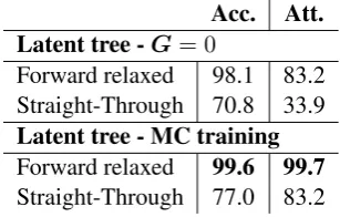
5.3 Results

The attachment scores and the tagging accuracy are provided in Table 1. We draw two conclu-sions from these results. First, using the ST esti-mator hurts performance, even though we do not relax at test time. Second, the MC approxima-tions, unlike the non-stochastic model, produces latent structures almost identical to gold trees. The non-stochastic version is however relatively suc-cessful in terms of tagging accuracy: we hypothe-size that the LSTM model solved the problem and

7_{To put it clearly, we have two sets of learned}

embed-dings: a set of lexicalized embeddings used for the input of the BiLSTM and a single unlexicalized embedding used for the input of the GCN.

* (max 3 4 (med 9 3 ) 1 )

- 4 - - 2

-Figure 2: An example from the ListOps dataset. Num-bers below operation tokens are valencies. (top)the original unlabelled phrase-structure. (bottom)our de-pendency conversion: each dede-pendency represents ei-ther an operand to argument relation or a closing paren-thesis relation.

Acc. Att. Latent tree -G= 0

Forward relaxed 98.1 83.2 Straight-Through 70.8 33.9

Latent tree - MC training

Forward relaxed 99.6 99.7

Straight-Through 77.0 83.2

Table 1: ListOps results: tagging accuracy (Acc.) and attachment score for the latent tree grammar (Att.).

uses trees as messages to communicate solutions. See extra analysis in App.C.8

6 Real-world Experiments

We evaluate our method on two real-world prob-lems: a sentence comparison task (natural lan-guage inference, see Section 6.1) and a sen-tence classification problem (sentiment classifica-tion, see Section 6.2). Besides using the differ-entiable dynamic programming method, our ap-proach also differs from previous work in that we use GCNs followed by a pooling operation, whereas most previous work used Tree-LSTMs. Unlike Tree-LSTMs, GCNs are trivial to paral-lelize over batches on GPU.

6.1 Natural Language Inference

The Natural Language Inference (NLI) problem is a task developed to test sentence understanding ca-pacity. Given a premise sentence and a hypothe-sis sentence, the goal is to predict a relation be-tween them: entailment, neutral or contradiction. We evaluate on the Stanford NLI (SNLI) and the

8

Acc. #Params

Yogatama et al.(2017)

*100D SPINN 80.5 2.3M

Maillard et al.(2017)

LSTM 81.2 161K

*Latent Tree-LSTM 81.6 231K

Kim et al.(2017)

No Intra Attention 85.8

-Simple -Simple Att. 86.2

-*Structured Attention 86.8

-Choi et al.(2018)

*100D ST Gumbel Tree 82.6 262K *300D ST Gumbel Tree 85.6 2.9M *600D ST Gumbel Tree 86.0 10.3M

Niculae et al.(2018)

Left-to-right Trees 81.0

-Flat 81.7

-Treebank 81.7

-*SparseMAP 81.9

-Liu and Lapata(2018)

175D No Attention 85.3 600K

*100D Projective Att. 86.8 1.2M *175D Non-projective Att. 86.9 1.1M

This work

No Intra Attention 84.4 382K

Simple Intra Att. 83.8 582K

*Latent Tree + 1 GCN 85.2 703K *Latent Tree + 2 GCN 86.2 1M

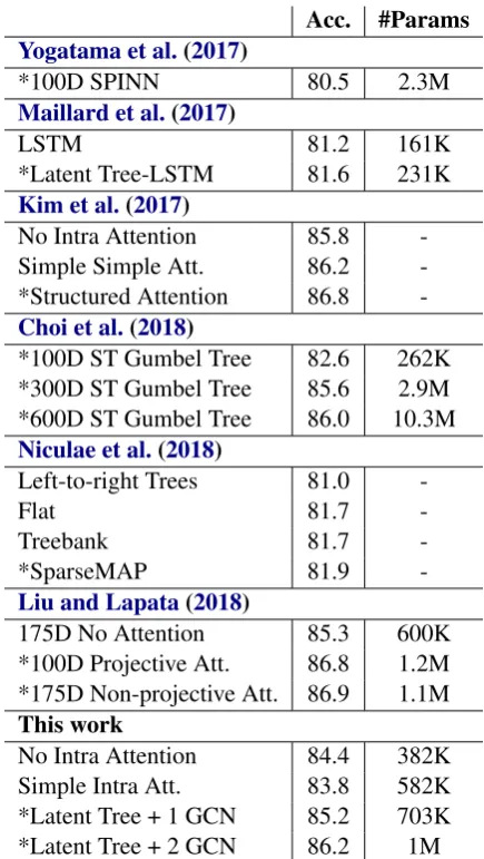
Table 2: SNLI results and number of network param-eters (discarding word embeddings). Stars indicate la-tent tree models.

Multi-genre NLI (MultiNLI) datasets. Our net-work is based on the decomposable attention (DA) model of Parikh et al. (2016). We induce struc-ture of both the premise and the hypothesis (see Equation1and Figure1b). Then, we run a GCN over the tree structures followed by inter-sentence attention. Finally, we apply max-pooling for each sentence and feed both sentence embeddings into a MLP to predict the label. Intuitively, using GCNs yields a form of intra-attention. See the hyper-parameters in AppendixA.2.

SNLI:The dataset contains almost 0.5m train-ing instances extracted from image captions ( Bow-man et al.,2015). We report results in Table2.

Our model outperforms both no intra-attention and simple intra-attention baselines9 with 1 layer

9_{The attention weights are computed in the same way as}

scores for tree prediction, i.e. using Equation1.

of GCN (+0.8) or two layers (+1.8). The im-provements with using multiple GCN hops, here and on MultiNLI (Table3b), suggest that higher-order information is beneficial.10 It is hard to com-pare different tree induction methods as they build on top of different baselines, however, it is clear that our model delivers results comparable with most accurate tree induction methods (Kim et al.,

2017;Liu and Lapata,2018). The improvements from using latent structure exceed these reported in previous work.

MultiNLI:MultiNLI is a broad-coverage NLI corpusWilliams et al.(2018b): the sentence pairs originate from 5 different genres of written and spoken English. This dataset is particularly inter-esting because sentences are longer than in SNLI, making it more challenging for baseline models.11 We follow the evaluation setting inWilliams et al.

(2018b,a): we include the SNLI training data, use the matched development set for early stopping and evaluate on the matched test set. We use the same network and parameters as for SNLI. We re-port results in Table3b.

The DA baseline (‘No Intra Attention’) per-forms slightly better (+0.6%) than the original BiLSTM baseline. Our latent tree model signifi-cantly improves over our the baseline, either with a single layer GCN (+3.4%) or with a 2-layer GCN (+4.9%). We observe a larger gap than on SNLI, which is expected given that MultiNLI is more complex. We perform extra ablation tests on MultiNLI in Section6.3.

6.2 Sentiment Classification

We experiment on the Stanford Sentiment Classi-fication dataset (Socher et al.,2013). The original dataset contains predicted constituency structure with manual sentiment labeling for each phrase. By definition, latent tree models cannot use the internal phrase annotation. We follow the setting ofNiculae et al. (2018) and compare to them in two set-ups: (1) with syntactic dependency trees predicted by CoreNLP (Manning et al.,2014); (2) with latent dependency trees. Results are reported in Table3a.

First, we observe that the bag of bigrams

base-10_{In contrast, multiple hops relying on edge marginals was}

not beneficial (Liu and Lapata,2018), personal communica-tion.

11_{The average sentence length in SNLI (resp. MultiNLI)}

(a)

Socher et al.(2013)

Bigram 83.1

Naive Bayes

Niculae et al.(2018)

CoreNLP 83.2

*Latent tree 84.7

This work

CoreNLP 83.8

*Latent tree 84.6

(b)

Acc.

Williams et al.(2018a)

300D LSTM 69.1

*300D SPINN 66.9

300D Balanced Trees 68.2 *300D ST Gumbel Tree 69.5

*300D RL-SPINN 67.3

This work

No Intra Attention 68.1 *Latent tree + 1 GCN 71.5 *Latent tree + 2 GCN 73.0

(c)

Match Mis. Baselines

No Intra Att 68.5 68.9 Simple Intra Att 67.9 68.4

Left-to-right trees

1 GCN 71.2 71.8

2 GCN 72.3 71.1

Latent head selection model

1 GCN 69.0 69.4

2 GCN 68.7 69.6

Latent tree model

1 GCN 71.9 71.7

2 GCN 73.2 72.9

Table 3:(a)SST results. Stars indicate latent tree models.(b)MultiNLI results. Stars indicate latent tree models. (c)Ablation tests on MultiNLI (results on the matched and mismatched development sets).

* My favorite restaurants are always at least a hundred miles away from my house .

* We do n’t loan a lot of money .

* He had recently seen pictures depicting those things .

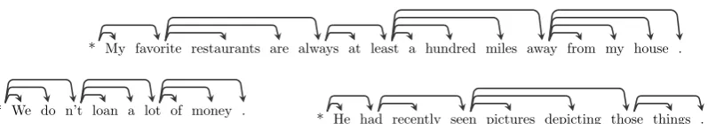
Figure 3: Examples of trees induced on the matched development set of MultiNLI, the model using 2 GCN layers.

line ofSocher et al. (2013) achieves results com-parable to all structured models. This suggest that the dataset may not be well suited for eval-uating structure induction methods. Our latent dependency model slighty improves (+0.8) over the CoreNLP baseline. However, we observe that while our baseline is better than the one ofNiculae et al. (2018), their latent tree model slightly out-performs ours (+0.1). We hypothesize that graph convolutions may not be optimal for this task.

6.3 Analysis

(Ablations)In order to test if the tree constraint is important, we do ablations on MultiNLI with two models: one with a latent projective tree variable (i.e. our full model) and one with a latent head se-lection model that does not impose any constraints on the structure. The estimation approach and the model are identical, except for the lack of the tree constraint (and hence dynamic programming) in the ablated model. We report results on develop-ment sets in Table3c. We observe that the latent tree models outperform the alternatives.

Previous work (e.g., Niculae et al., 2018) in-cluded comparison with balanced trees, flat trees

and left-to-right (or right-to-left) chains. Flat trees are pointless with the GCN + DA combination: the corresponding pooling operation is already done in DA. Though balanced trees are natural with bottom-up computation of TreeLSTMs, for GCNs they would result in embedding essentially ran-dom subsets of words. Consequently, we com-pare only to left-to-right chains of dependencies.12 This approach is substantially less accurate than our methods, especially for out-of-domain (i.e. mismatched) data.

(Grammar) We also investigate the structure of the induced grammar. We report the latent struc-ture of three sentences in Figure 3. We observe that sentences are divided into spans, where each span is represented with a series of left depen-dencies. Surprisingly, the model chooses to use only left-to-right dependencies. The neural net-work does not include a RNN layer, so this may suggest that the grammar is trying to reproduce an recurrent model while also segmenting the sen-tence in phrases.

(Speed)We use a_O(n3_{)-time parsing algorithm.}

12_{They are the same as right-to-left ones, as our GCNs treat}

Nevertheless, our model is efficient: one epoch on SNLI takes 470 seconds, only 140 seconds longer than with the _O(n2_{)-time latent-head} ver-sion of our model (roughly equivalent to classic self-attention). The latter model is computed on GPU (Titan X) while ours uses CPU (Xeon E5-2620) for the dynamic program and GPU for run-ning the rest of the network.

7 Related work

Recently, there has been growing interest in pro-viding an inductive bias in neural network by forc-ing layers to represent tree structures (Kim et al.,

2017;Maillard et al.,2017;Choi et al.,2018; Nic-ulae et al.,2018;Williams et al., 2018a;Liu and Lapata, 2018). Maillard et al. (2017) also op-erates on a chart but, rather than modeling dis-crete trees, uses a soft-gating approach to mix representations of constituents in each given cell. While these models showed consistent improve-ment over comparable baselines, they do not seem to explicitly capture syntactic or semantic struc-tures (Williams et al., 2018a). Nangia and Bow-man(2018) introduced the ListOps task where the latent structure is essential to predict correctly the downstream prediction. Surprisingly, the models ofWilliams et al.(2018a) andChoi et al. (2018) failed. Much recent work in this context relies on latent variables, though we are not aware of any work closely related to ours. Differentiable structured layers in neural networks have been ex-plored for semi-supervised parsing, for example by learning an auxiliary task on unlabelled data (Peng et al., 2018) or using a variational autoen-coder (Corro and Titov,2019).

Besides research focused on inducing task-specific structures, another line of work, grammar induction, focused on unsupervised induction of linguistic structures. These methods typically rely on unlabeled texts and are evaluated by comparing the induced structures to actual syntactic annota-tion (Klein and Manning,2005;Shen et al.,2018;

Htut et al.,2018).

8 Conclusions

We introduced a novel approach to latent tree learning: a relaxed version of stochastic dif-ferentiable dynamic programming which allows for efficient sampling of projective dependency trees and enables end-to-end differentiation. We demonstrate effectiveness of our approach on both

synthetic and real tasks. The analyses confirm im-portance of the tree constraint. Future work will investigate constituency structures and new neural architectures for latent structure incorporation.

Acknowledgments

We thank Maximin Coavoux and Serhii Havrylov for their comments and suggestions. We are grateful to Vlad Niculae for the help with pre-processing the SST data. We also thank the anonymous reviewers for their comments. The project was supported by the Dutch National Sci-ence Foundation (NWO VIDI 639.022.518) and European Research Council (ERC Starting Grant BroadSem 678254).

References

Joost Bastings, Ivan Titov, Wilker Aziz, Diego Marcheggiani, and Khalil Simaan. 2017. Graph convolutional encoders for syntax-aware neural ma-chine translation. InProceedings of the 2017 Con-ference on Empirical Methods in Natural Language Processing, pages 1947–1957. Association for Com-putational Linguistics.

Yoshua Bengio. 2013. Estimating or propagating gra-dients through stochastic neurons. arXiv preprint arXiv:1305.2982.

Samuel R. Bowman, Gabor Angeli, Christopher Potts, and Christopher D. Manning. 2015. A large anno-tated corpus for learning natural language inference. In Proceedings of the 2015 Conference on Empiri-cal Methods in Natural Language Processing, pages 632–642. Association for Computational Linguis-tics.

Stephen Boyd and Lieven Vandenberghe. 2004. Con-vex optimization. Cambridge university press.

Jihun Choi, Kang Min Yoo, and Sang-goo Lee. 2018. Learning to compose task-specific tree structures. InProceedings of the 2018 Association for the Ad-vancement of Artificial Intelligence (AAAI). and the 7th International Joint Conference on Natural Lan-guage Processing (ACL-IJCNLP).

Caio Corro and Ivan Titov. 2019. Differentiable perturb-and-parse: Semi-supervised parsing with a structured variational autoencoder. InProceedings of the International Conference on Learning Repre-sentations.

D Den Hertog, Cornelis Roos, and Tam´as Terlaky. 1994. Inverse barrier methods for linear program-ming. RAIRO-Operations Research, 28(2):135– 163.

Jason M. Eisner. 1996.Three new probabilistic models for dependency parsing: An exploration. In COL-ING 1996 Volume 1: The 16th International Confer-ence on Computational Linguistics.

Jennifer Foster, ¨Ozlem C¸ etinoglu, Joachim Wagner, Joseph Le Roux, Stephen Hogan, Joakim Nivre, Deirdre Hogan, and Josef Van Genabith. 2011. # hardtoparse: Pos tagging and parsing the twitter-verse. InAAAI 2011 workshop on analyzing micro-text, pages 20–25.

Michael C Fu. 2006. Gradient estimation. Hand-books in operations research and management sci-ence, 13:575–616.

Stephen Gould, Basura Fernando, Anoop Cherian, Pe-ter Anderson, Rodrigo Santa Cruz, and Edison Guo. 2016. On differentiating parameterized argmin and argmax problems with application to bi-level opti-mization. arXiv preprint arXiv:1607.05447.

Phu Mon Htut, Kyunghyun Cho, and Samuel Bow-man. 2018. Grammar induction with neural lan-guage models: An unusual replication. In Proceed-ings of the 2018 Conference on Empirical Methods in Natural Language Processing, pages 4998–5003. Association for Computational Linguistics.

Eric Jang, Shixiang Gu, and Ben Poole. 2017. Cate-gorical reparameterization with gumbel-softmax. In

Proceedings of the 2017 International Conference on Learning Representations.

Yoon Kim, Carl Denton, Luong Hoang, and Alexan-der M Rush. 2017. Structured attention networks. In Proceedings of the International Conference on Learning Representations.

Diederik P Kingma and Max Welling. 2014. Auto-encoding variational bayes. InProceedings of the International Conference on Learning Representa-tions.

Thomas N Kipf and Max Welling. 2017. Semi-supervised classification with graph convolutional networks. InProceedings of the International Con-ference on Learning Representations.

Dan Klein and Christopher D Manning. 2005. The un-supervised learning of natural language structure. Stanford University Stanford, CA.

John Lafferty, Andrew McCallum, and Fernando CN Pereira. 2001. Conditional random fields: Prob-abilistic models for segmenting and labeling se-quence data. In Proceedings of the 18th Interna-tional Conference on Machine Learning.

Yang Liu and Mirella Lapata. 2018. Learning struc-tured text representations.Transactions of the Asso-ciation for Computational Linguistics, 6:63–75.

Yang Liu, Furu Wei, Sujian Li, Heng Ji, Ming Zhou, and Houfeng WANG. 2015. A dependency-based neural network for relation classification. In Pro-ceedings of the 53rd Annual Meeting of the Associ-ation for ComputAssoci-ational Linguistics and the 7th In-ternational Joint Conference on Natural Language Processing (Volume 2: Short Papers), pages 285– 290. Association for Computational Linguistics.

Chris J Maddison, Daniel Tarlow, and Tom Minka. 2014. A* sampling. In Advances in Neural Infor-mation Processing Systems, pages 3086–3094.

Jean Maillard, Stephen Clark, and Dani Yogatama. 2017. Jointly learning sentence embeddings and syntax with unsupervised tree-LSTMs. arXiv preprint arXiv:1705.09189.

Christopher Manning, Mihai Surdeanu, John Bauer, Jenny Finkel, Steven Bethard, and David McClosky. 2014. The stanford corenlp natural language pro-cessing toolkit. In Proceedings of 52nd Annual Meeting of the Association for Computational Lin-guistics: System Demonstrations, pages 55–60. As-sociation for Computational Linguistics.

Diego Marcheggiani and Ivan Titov. 2017. Encoding sentences with graph convolutional networks for se-mantic role labeling. In Proceedings of the 2017 Conference on Empirical Methods in Natural Lan-guage Processing, pages 1507–1516. Association for Computational Linguistics.

Arthur Mensch and Mathieu Blondel. 2018. Differen-tiable dynamic programming for structured predic-tion and attenpredic-tion. InProceedings of the 35th Inter-national Conference on Machine Learning.

Nikita Nangia and Samuel Bowman. 2018. Listops: A diagnostic dataset for latent tree learning. In Pro-ceedings of the 2018 Conference of the North Amer-ican Chapter of the Association for Computational Linguistics: Student Research Workshop, pages 92– 99. Association for Computational Linguistics.

Jason Naradowsky, Sebastian Riedel, and David Smith. 2012. Improving NLP through marginalization of hidden syntactic structure. In Proceedings of the 2012 Joint Conference on Empirical Methods in Natural Language Processing and Computational Natural Language Learning, pages 810–820, Jeju Island, Korea. Association for Computational Lin-guistics.

Vlad Niculae, Andr´e F. T. Martins, and Claire Cardie. 2018. Towards dynamic computation graphs via sparse latent structure. InProceedings of the 2018 Conference on Empirical Methods in Natural Lan-guage Processing, pages 905–911. Association for Computational Linguistics.

George Papandreou and Alan L Yuille. 2011. Perturb-and-MAP random fields: Using discrete optimiza-tion to learn and sample from energy models. In

Computer Vision (ICCV), 2011 IEEE International Conference on, pages 193–200. IEEE.

Ankur Parikh, Oscar T¨ackstr¨om, Dipanjan Das, and Jakob Uszkoreit. 2016. A decomposable attention model for natural language inference. In Proceed-ings of the 2016 Conference on Empirical Methods in Natural Language Processing, pages 2249–2255. Association for Computational Linguistics.

Hao Peng, Sam Thomson, and Noah A. Smith. 2018.

Backpropagating through structured argmax using a spigot. In Proceedings of the 56th Annual Meet-ing of the Association for Computational LMeet-inguistics (Volume 1: Long Papers), pages 1863–1873. Asso-ciation for Computational Linguistics.

Slav Petrov, Pi-Chuan Chang, Michael Ringgaard, and Hiyan Alshawi. 2010. Uptraining for accurate de-terministic question parsing. InProceedings of the 2010 Conference on Empirical Methods in Natural Language Processing, pages 705–713. Association for Computational Linguistics.

Florian A Potra and Stephen J Wright. 2000. Interior-point methods. Journal of Computational and Ap-plied Mathematics, 124(1-2):281–302.

Anand Rangarajan. 2000. Self-annealing and self-annihilation: unifying deterministic anneal-ing and relaxation labelanneal-ing. Pattern Recognition, 33(4):635–649.

John Schulman, Nicolas Heess, Theophane Weber, and Pieter Abbeel. 2015. Gradient estimation using stochastic computation graphs. InAdvances in Neu-ral Information Processing Systems, pages 3528– 3536.

Yikang Shen, Zhouhan Lin, Chin wei Huang, and Aaron Courville. 2018. Neural language modeling by jointly learning syntax and lexicon. In Interna-tional Conference on Learning Representations.

Richard Socher, Alex Perelygin, Jean Wu, Jason Chuang, Christopher D. Manning, Andrew Ng, and Christopher Potts. 2013. Recursive deep models for semantic compositionality over a sentiment tree-bank. In Proceedings of the 2013 Conference on Empirical Methods in Natural Language Process-ing, pages 1631–1642. Association for Computa-tional Linguistics.

Xinyi Wang, Hieu Pham, Pengcheng Yin, and Graham Neubig. 2018. A tree-based decoder for neural ma-chine translation. InProceedings of the 2018 Con-ference on Empirical Methods in Natural Language

Processing, pages 4772–4777. Association for Com-putational Linguistics.

Adina Williams, Andrew Drozdov, and Samuel R. Bowman. 2018a. Do latent tree learning models identify meaningful structure in sentences? Trans-actions of the Association for Computational Lin-guistics, 6:253–267.

Adina Williams, Nikita Nangia, and Samuel Bowman. 2018b. A broad-coverage challenge corpus for sen-tence understanding through inference. In Proceed-ings of the 2018 Conference of the North American Chapter of the Association for Computational Lin-guistics: Human Language Technologies, Volume 1 (Long Papers), pages 1112–1122. Association for Computational Linguistics.

R Williams. 1987. A class of gradient-estimation al-gorithms for reinforcement learning in neural net-works. InProceedings of the International Confer-ence on Neural Networks, pages II–601.

A Neural Parametrization

(Implementation) We implemented our neural networks with the C++ API of the Dynet library (Neubig et al., 2017). The continuous relaxation of the parsing algorithm is implemented as a cus-tom computation node.

(Training) All networks are trained with Adam initialized with a learning rate of 0.0001 and batches of size 64. If the dev score did not im-prove in the last 5 iterations, we multiply the learn-ing rate by0.9and load the best known model on dev. For the ListOps task, we run a maximum of 100 epochs, with exactly 100 updates per epoch. For NLI and SST tasks, we run a maximum of 200 epochs, with exactly 8500 and 100 updates per epoch, respectively.

All MLPs and GCNs have a dropout ratio of 0.2except for the ListOps task where there is no dropout. We clip the gradient if its norm exceed5.

A.1 ListOps Valency Tagging

(Dependency Parser) Embeddings are of size 100. The BiLSTM is composed of two stacks (i.e. we first run a left-to-right and a right-to-left LSTM, then we concatenate their outputs and fi-nally run a left-to-right and a right-to-left LSTM again) with one single hidden layer of size 100. The initial state of the LSTMs are fixed to zero.

The MLPs of the dotted attention have 2 layers of size 100 and aReLUactivation function

(Tagger) The unique embedding is of size 100. The GCN has a single layer of size 100 and a ReLU activation. Then, the tagger is composed of a MLP with a layer of size 100 and a ReLU activation followed by a linear projection into the output space (i.e. no bias, no non-linearity).

A.2 Natural Language Inference

All activation functions are ReLU. The inter-attention part and the classifier are exactly the same than in the model ofParikh et al.(2016).

(Embeddings) Word embeddings of size 300 are initialized with Glove and are not updated dur-ing traindur-ing. We initialize 100 unknown word em-beddings where each value is sampled from the normal distribution. Unknown words are mapped using a hashing method.

(GCN) The embeddings are first passed through a one layer MLP with an output size of 200. The

dotted attention is computed by two MLP with two layers of size 200 each. Functionf(),g()andh() in the GCN layers are one layer MLPs without ac-tivation function. The σ activation function of a GCN isReLU. We use dense connections for the GCN.

A.3 Sentiment Classification

(Embeddings) We use Glove embeddings of size 300. We learn the unknown word embed-dings. Then, we compute context sensitive em-beddings with a single-stack/single-layer BiLSTM with a hidden-layer of size 100.

(GCN) The dotted attention is computed by two MLP with one layer of size 300 each. There is no distance bias in this model. Functionf(),g()and

h()in the GCN layers are one layer MLPs without activation function. Theσ activation function of a GCN isReLU. We do not use dense connections in this model.

(Output) We use a max-pooling operation on the GCN outputs followed by an single-layer MLP of size 300.

B Illustration of the Continuous Relaxation

Too give an intuition of the continuous relaxation, we plot the arg max function and the penalized arg maxin Figure4. We plot the first output for input(x1, x2,0).

C ListOps Training

We plot tagging accuracy and attachment score with respect to the training epoch in Figure5. On the one hand, we observe that the non-stochastic versions converges way faster in both metrics: we suspect that it develops an alternative protocol to pass information about valencies from LSTM to the GCN. On the other hand, MC sampling may have a better exploration of the search space but it is slower to converge.

We stress that training with MC estimation re-sults in the latent tree corresponding (almost) per-fectly to the gold grammar.

D Fast differentiable dynamic program implementation

(a)

−2 0

2

−2 0 2 0 0.5 1

(b)

−2 0

2

−2 0 2 0 0.5 1

Figure 4: (a)Single output of an arg maxfunction. The derivative is null almost everywhere, i.e. there is no descent direction.(b)Single output of the differentiable relaxation. The derivatives are non-null.

(a) Accuracy

0 20 40 60 80 100

0 20 40 60 80 100

epoch

accurac

y

(b) Attachment score

0 20 40 60 80 100

0 20 40 60 80 100

epoch

attachment

score